Postprint
This is the accepted version of a paper presented at International Conference On Computational Science,
ICCS 2015 Computational Science at the Gates of Nature.
Citation for the original published paper:
Aguilar, X., Fürlinger, K., Laure, E. (2015)
Visual MPI Performance Analysis using Event Flow Graphs.
In: Procedia Computer Science (pp. 1353-1362).
http://dx.doi.org/10.1016/j.procs.2015.05.322
N.B. When citing this work, cite the original published paper.
Permanent link to this version:
This space is reserved for the Procedia header, do not use it
Visual MPI Performance Analysis using Event Flow Graphs
Xavier Aguilar
1, Karl F¨
urlinger
2, and Erwin Laure
11
KTH Royal Institute of Technology, High Performance Computing and Visualization Department (HPCViz), and Swedish e-Science Research Center (SeRC)
{xaguilar, erwinl}@pdc.kth.se
2
Ludwig-Maximilians-Universit¨at (LMU) Munich, Computer Science Department, MNM Team
Karl.Fuerlinger@nm.ifi.lmu.de
Abstract
Event flow graphs used in the context of performance monitoring combine the scalability and low overhead of profiling methods with lossless information recording of tracing tools. In other words, they capture statistics on the performance behavior of parallel applications while pre-serving the temporal ordering of events. Event flow graphs require significantly less storage than regular event traces and can still be used to recover the full ordered sequence of events performed by the application.
In this paper we explore the usage of event flow graphs in the context of visual performance analysis. We show that graphs can be used to quickly spot performance problems, helping to better understand the behavior of an application. We demonstrate our performance analysis approach with MiniFE, a mini-application that mimics the key performance aspects of finite-element applications in High Performance Computing (HPC).
Keywords: visual performance analysis, event flow graphs, loop detection, MPI monitoring
1
Introduction
Comprehending software behavior is getting more important as systems increase the parallelism and heterogeneity of their resources. Nowadays, application development and tuning to reach system peak performance is becoming a heroic task. Therefore, visual performance analysis techniques to easily understand application behavior are an essential part of the HPC domain. Performance visualization is the process of mapping performance data onto graphical dis-plays in order to analyze it. For instance, mapping resource utilization into program structure using different charts and timeline views. The scalability and usability of performance vi-sualization tools are closely related to the amount of data collected, in other words, to the
approach used when monitoring a running application via tracing or profiling. Tracing con-sists in generating huge logs of time-stamped events that provide detailed information on each single application event. On the other hand, profiling generates easy to understand reports with aggregate data and program trends, usually discarding the temporal nature of the data kept in time-stamped traces. Therefore, profiling introduces less perturbation into monitored applications and is more scalable than tracing.
In [6, 2] the authors presented a novel approach for performance monitoring of parallel applications using event flow graphs in conjunction with the IPM monitoring tool. This new approach combines the low overhead and good scalability of profiling but preserves the temporal ordering of the events as in tracing. The first experiments showed promising results, proving this new approach as a good solution for MPI trace compression. This paper now explores the usability of event flow graphs together with automatic cycle detection and graph coloring in the task of visual performance analysis of MPI parallel applications. The utilization of this new visual approach is presented with a case study using a finite-element code.
The rest of this paper is structured as follows: In Section 2 we present some background of our approach on the use of event flow graphs for MPI monitoring. Section 3 shows our visual-ization framework and its strategies to help in the task of performance analysis visualvisual-ization. In Section 4 we demonstrate the use of event flow graphs analyzing a finite-element code. We review related work in performance analysis visualization in Section 5. The paper ends with future work and conclusions in Section 6 and Section 7, respectively.
2
Event Flow Graphs
As mentioned in Section 1, the IPM monitoring tool has recently been extended in order to capture and generate event flow graphs of MPI parallel applications. For each MPI rank, IPM generates a directed graph in which nodes represent the MPI calls performed by that process and edges are the transitions between the MPI calls. In other words, edges in the graph represent the computation phases performed by an application between two consecutive MPI calls. Therefore, event flow graphs keep the temporal structure of the data without storing any explicit time information such as timestamps.
The flow graphs captured by IPM are directed multidigraphs, that is, directed graphs with more than one edge between the same two nodes. These multiple edges between the same two nodes have sequence numbers associated representing their execution order. Using this information, the complete sequence of events performed by the application can be recovered simply by traversing the graph from the initial node following the edges in ascending order. Furthermore, each graph element has several performance metrics associated. For instance, nodes in the graph record the number of occurrences and total execution time, as well as several other metrics related to the MPI call they represent such as transfer size or communication partner rank. Hence, we can generate a performance profile of the application with added information about the temporal nature of its events. Detailed information on how graphs are generated, and used for trace reconstruction can be found in [2].
3
Graph visualization
The event flow graphs generated by IPM can be stored in DOT graph format [11] and visualized with tools such as GraphViz [5]. In addition, we have developed a framework that generates
Visual MPI Performance Analysis using Event Flow Graphs Aguilar, F¨urlinger, and Laure
the analysis reports presented in the following subsections in the form of HTML pages that can be viewed with any web browser.
One of the main causes hindering graph exploration is graph order, that is, the number of nodes. Our experiments in [2] showed that the graphs obtained from several scientific applica-tions from the NERSC Benchmark Suite often had hundreds of nodes. Thus, it is essential to utilize methods to reduce the complexity of such graphs for visual exploration.
In the following subsections, we present two techniques to enable and simplify graph explo-ration for performance analysis: automatic loop detection and compression, and graph coloring.
3.1
Loop detection
The vast majority of scientific parallel applications are iterative, that is, they consist of one or more loops in which typically most of the time is spent. If an application has loops that contain MPI calls, then its corresponding flow graph will contain cycles. By searching for cycles, processing them, and replacing them with loop nodes, graphs can be simplified and user attention can be directed to the most interesting sections.
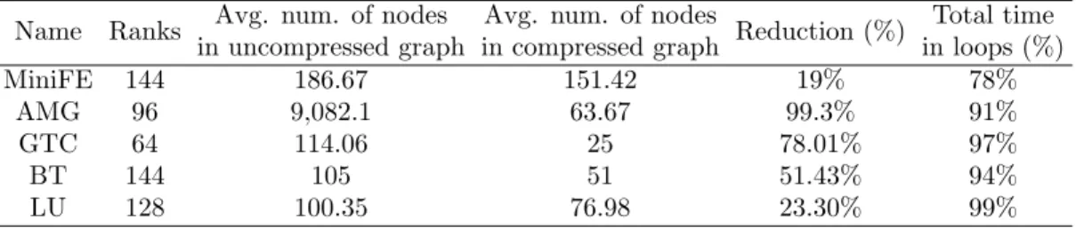
Once a cycle is detected, its nodes are compressed into a single node in the graph, and for each loop node, a new hyper-linked subgraph is generated containing only the nodes and edges corresponding to that loop. If this subgraph contains further cycles, the process is repeated and new subgraphs are generated for those nested loops as well. Loop nodes and their nesting increase graph readability by reducing the number of nodes in a graph and by directly corre-sponding to the application loop structure. Table 1 provides the reduction in the number of nodes for the top-level graph achieved when applying automatic loop compression to several applications from the Trinity Benchmark Suite and the NAS Parallel Benchmarks. As IPM generates one graph per MPI process, the table contains the average number of nodes for all the graphs within each application. We can see in the table that we achieve at least a 20% reduction on the graph size by automatically detecting cycles and replacing them with loop nodes. In addition, as compressed graphs are sequential since all their cycles are collapsed into single nodes, and as those nodes are represented with a different shape, the process of spotting what are the interesting parts in the graph that need further investigation becomes an easy task.
Name Ranks Avg. num. of nodes in uncompressed graph
Avg. num. of nodes
in compressed graph Reduction (%)
Total time in loops (%) MiniFE 144 186.67 151.42 19% 78% AMG 96 9,082.1 63.67 99.3% 91% GTC 64 114.06 25 78.01% 97% BT 144 105 51 51.43% 94% LU 128 100.35 76.98 23.30% 99%
Table 1: Graph statistics on the number of nodes and loop time for several MPI applications. Loop nodes in graphs are also useful to summarize statistics as they can show accumulated values from their corresponding subgraphs. For instance, accumulated time spent in every node and edge. Thus, facilitating the task of finding where most of the time is spent. Other metrics that can be accumulated and displayed on a per loop basis are transfer sizes and aggregated hardware counter metrics for example. Moreover, as we know the total number of iterations for one cycle in the graph, the tool can also show average statistics per iteration. The last column in Table 1 provides the average percentage of time contained in cycles (loops) over the total
graph time, that is, over the total execution time of each process. As can be observed in the table, the detected cycles account for most of the running time for each application.
Algorithms for cycle detection in graphs have been studied for years [16, 9, 18]. Our graph visualization framework implements the algorithm in [20]. This algorithm traverses the graph only once with a depth-first search (DFS) and runs in almost linear time. In addition, it is easy to implement because it does not need any complicated data structures as most of the other cycle detection algorithms do. More details on the detection of loops, and event flow graph analysis could be found in an upcoming paper.
3.2
Graph coloring
As previously mentioned, performance metrics can be associated with different elements in the graphs. Nodes, which represent MPI calls performed by the process, can store total time, maximum and minimum time, number of occurrences, and total number of bytes transferred. For the edges, which are transitions between MPI calls, or in other words, computation phases between two MPI calls, timings and hardware counters using the PAPI interface [13] can be collected and saved.
These performance metrics can be used to color the graph in order to highlight the most interesting parts of it. For example, coloring the nodes with a gradient to show the user in which MPI calls most of the time is spent, or coloring the edges using hardware counters data to show computational phases with bad single-core performance. Loop nodes representing collapsed cycles in the graph can similarly be colored by aggregate metrics.
Metrics that can be used for graph coloring in our current graph framework are time, bytes and number of occurrences for nodes; and time, instructions per cycle (IPC), million of instructions per second (MIPS), million of floating point operations per second (MFLOPS) and cache misses rate for edges.
4
Experiments
In this section we show how the utilization of event flow graphs during the performance analysis process can be helpful to spot performance problems. We run and analyze the MiniFE mini-application from the Mantevo project [10]. MiniFE is a finite-element code that assembles a sparse-linear system from the steady-state conduction in a 3D box modeled by hexahedral elements. It solves the linear-system using the un-preconditioned conjugate-gradient algorithm. We performed our experiments on a Cray XE6 system with 2 AMD Opteron Magny-Cours processors per node. The nodes had 32 GB DDR3 memory and were interconnected with a Cray Gemini network. MiniFE was compiled using Intel 12.1.5 and run on 144 cores with MPICH and the small test case provided in the benchmark distribution.
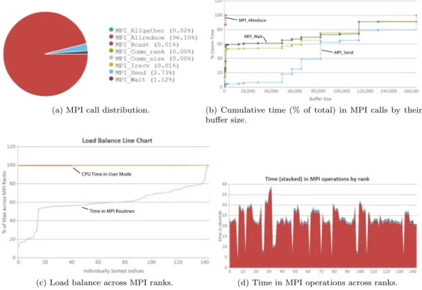
The test case used with MiniFE runs for a total of 133.8 seconds, spending around 17% of its time in MPI communication. Figure 1a shows the distribution of time in MPI calls. As we can see, the predominant operation is MPI Allreduce, followed by MPI Send and MPI Wait. Figure 1b shows the cumulative time distribution (% of total) for these three main MPI calls. The message sizes for MPI Allreduce (red line) are quite small, almost 87% of the time is spent transmitting messages of at most 8 bytes and the rest of the time is spent in 1KB messages. For MPI Send (blue), 80% of the time spent in the call is with messages up to 160KB.
Figure 1c shows the percentage of the maximum value of user time (CPU time in user mode) and MPI time across ranks, separately sorted from lowest to highest value. This type of display is best used to spot load imbalance among the MPI ranks. In our case user time is almost the
Visual MPI Performance Analysis using Event Flow Graphs Aguilar, F¨urlinger, and Laure
(a) MPI call distribution.
MPI_Allreduce MPI_Wait
MPI_Send
(b) Cumulative time (% of total) in MPI calls by their buffer size.
Time in MPI Routines CPU Time in User Mode
(c) Load balance across MPI ranks. (d) Time in MPI operations across ranks.
Figure 1: MPI statistics for MiniFE. Figures a, b, and d share the same color encoding.
same across ranks while the time spent in MPI varies significantly among processors. The chart shows four different trends in the MPI line. The first trend, the first 15 processes in the left part of the chart, have an MPI time around 15%-25% of the process with maximum MPI time. The second trend corresponds to processes with an MPI time oscillating between 50%-65% of the maximum MPI time. The third trend between 65% and 80%, and finally, there is a small group of few processes at the rightest part of the chart with the highest communication time.
Figure 1d shows the total MPI time broken down by MPI call in the y-axis with MPI processes ordered by rank number in the x-axis. Looking at the stacked times for each different MPI call across ranks we can again see the previously identified load imbalance. In addition, we can observe that most of the variation in the MPI time occurs within MPI Allreduce.
The previously presented plots have given us an overview of the overall performance behavior for the whole application. Now we can use our event flow graphs to zoom into a process level. By exploring the top-level graph for one of the ranks with long MPI time, we discover that most of the time for this MPI process is spent in a single loop node. Thereupon, we can open the subgraph for that loop node and check which events form that loop, their execution order and how the time is spent. Figure 2a shows the subgraph for that loop. The loop starts with an MPI Comm size operation, followed by a series of nested loops (round shaped nodes), and ends with two MPI Allreduce operations. By using the call site information provided by IPM we can map graph nodes to the source code. Those three nested loops are part of the function exchange externals() in which data between processes is interchanged. The subgraph for the
MPI_Comm_size cs=64 t=0.0007 Loop 13 (0.0416) 200 (0.01) Loop 14 (0.3966) 200 (0.37) Loop 15 (0.0583) 200 (0.002) MPI_Allreduce8B cs=68 t=31.6909 200 (59.07) MPI_Allreduce 8B cs=69 t=1.1559 199 (7.55) 199 (3.35)
(a) Most time-consuming loop in MiniFE for one of the processes with long total MPI time.
MPI_Comm_size cs=64 t=0.0005 Loop 12 (0.0224) 200 (0.01) Loop 13 (0.2896) 200 (0.37) Loop 14 (0.0178) 200 (0.002) MPI_Allreduce 8B cs=68 t=0.7074 200 (90.12) MPI_Allreduce 8B cs=69 t=0.4822 199 (8.22) 199 (3.45)
(b) Most time-consuming loop in MiniFE for one of the processes with short total MPI time.
Figure 2: Main program loop for two different MiniFE MPI processes. Nodes and edges are colored by time from yellow (low value) to red (high value).
first nested loop (Loop 13 ) shows that the process iterates over all its neighbors posting non-blocking receives (MPI Irecv). Then, the process sends data to all its neighbors (MPI Send) in the second inner loop (Loop 14 ). In the third nested loop (Loop 15 ), the process waits for the data from its neighbors (MPI Wait). The graph in Figure 2a is colored using time with a gradient ranging from yellow (low values) to red (high values). Thus, we can easily identify how the time is spent in the graph. As we can see highlighted in the figure, most of the time for this graph is spent in the edge between Loop 15 and the MPI Allreduce with call site 68. In other words, the time is spent in the computation performed between the last MPI Wait within Loop 15 and the MPI Allreduce. The rest of the time for the graph is mainly spent in the MPI Allreduce with call site 68 following that computation.
Using again the call sites and the call path information provided by IPM we can locate which part of the source code corresponds to the edge that contains most of the time for the loop. The edge is the sparse matrix vector multiplication (SpMV) code within the conjugate gradient function. This operation is implemented in MiniFE using a naive algorithm and should be optimized because it is an expensive operation performed on each iteration of the conjugate gradient calculation. It could be optimized by using specialized libraries such as PETSc (the Portable, Extensible Toolkit for Scientific Computation) or more optimized algorithms for the SpMV operation such as the work in [21]. Nevertheless, the optimization of the code is out of the scope of this paper.
The graph in Figure 2a corresponds to a process with long MPI time (a fast process). Now we can explore the graph for one of the processes with short total MPI time (a slow process) in order to compare how they differ. The top-level graphs for these two processes are very similar, however, their subgraphs for the loop with the highest accumulated time differ in the distribution of such time across nodes and edges. More specifically, in the section of the subgraph related to the sparse matrix vector multiplication. Figure 2b shows that the slow process spends most of its time in the computation of the SpMV operation.
By looking at Figure 2a and Figure 2b, it is easy to discern what is the cause of the overall imbalance previously detected in the application. The fast process from Figure 2a finishes the SpMV operation quicker and spends a lot of time waiting for slow processes such as the one from Figure 2b at the MPI Allreduce call. The profiles generated by IPM confirm that the process in Figure 2b receives in total 32MB more of data than the other process during the whole execution, around 38,000 matrix lines more per iteration.
As previously explained in Section 3.2, graphs can also be colored by hardware counter values. In our experiments we used PAPI to collect instructions, cycles, floating-point operations
Visual MPI Performance Analysis using Event Flow Graphs Aguilar, F¨urlinger, and Laure MPI_Comm_size cs=64 t=0.0007 Loop 13 (0.0416) 0.09 0.22 (0.3966)Loop 14 0.75 (0.0583)Loop 15 MPI_Allreduce 8B cs=68 t=31.6909 0.51 MPI_Allreduce 8B cs=69 t=1.1559 0.32 0.32
(a) Most time-consuming loop in MiniFE for one of the processes with long total MPI time.
MPI_Comm_size cs=64 t=0.0005 Loop 12 (0.0224) 0.12 0.16 (0.2896)Loop 13 0.75 (0.0178)Loop 14 MPI_Allreduce 8B cs=68 t=0.7074 0.34 MPI_Allreduce 8B cs=69 t=0.4822 0.30 0.32
(b) Most time-consuming loop in MiniFE for one of the processes with short total MPI time.
Figure 3: Main program loop for two different MiniFE MPI processes. Nodes are colored by time and edges by IPC (instructions per cycle). The gradient color goes from yellow (low value) to red (high value).
and data cache misses. Figure 3 shows the graphs of both processes with edges colored by instructions per cycle (IPC) and nodes colored by time. The edge labels depict the IPC values. The graphs show that while both processes have very similar IPC in almost all the edges, the process that spends more time in the SpMV operation (bottom graph) has 33% IPC less than the other process in that specific edge. Furthermore, looking at other hardware counters we also observed that for the process with lower IPC, its data cache misses are two times higher than for the other process.
In this section we have seen how graphs can help to better visualize and understand the be-havior of an application providing a sense of temporality between events. In addition, although the main focus of this paper is visual performance analysis, graphs are good data structures for MPI trace compression as demonstrated in [2]. In the case of MiniFE, the graphs used in this experiment had an average compression ratio of 19.93x with respect to regular full traces. In other words, we needed 20 times less space to store our event flow graphs than to store regular event traces of MiniFE generated also with IPM. Moreover, the overhead introduced into the application when capturing graphs is very small, never exceeding the 0.5% of total application running time for our test case.
5
Related Work
The performance tools community has been developing tools for HPC systems over the past twenty years. Therefore, users can choose over a broad variety of software from profilers using interrupt-based sampling to fine-grain tracers.
Paraver [15], Vampir [14], Jumpshot [22] and Paj´e [4] are performance visualization tools focused on post-mortem exploration of traces. They provide the highest possible level of detail keeping the temporal order of the data (events ordered in time with timestamps). However, they are complicated to use and have a steep learning curve. In addition, they lack scalability due to the huge amount of information that they have to deal with. For instance, exploring traces from applications with long running times or with high core counts becomes infeasible due to the large amount of data generated. Using graphs does not provide the same level of detail but it is a very easy-to-use method with almost no user involvement in the process of capturing and generating the graphs. Furthermore, it is scalable since graphs only keep statistics than
can be stored in small files. Thus, our current work can be used as a complement to those tracing tools, providing users with a first quick overview about the performance behavior of their applications. Hence, if users want fine-grained detail, they can use any of the previously cited frameworks to focus into some specific part of the code.
Our work is also related to profiling tools such as gprof [8] or mpiP [19]. These tools provide aggregated statistics with low overhead. However, their statistics can not capture any temporal phenomena in the data. For instance, they can show different metrics about function calls but not the temporal relations between them. In contrast, our event flow graphs allow us to provide the same type of aggregated statistics with the addition of the temporal order between events. Other tool frameworks such as HPCtoolkit [1], Scalasca [7] and TAU [17] support profiling and tracing at the same time. These toolkits provide different charts to easily explore the collected performance data, and relate it to the application source code. For instance, views on statistics per thread, call-path graphs, or Cartesian grids mapping metrics to system resources. As in the case with tracing toolkits, our approach can be used as a complement to the already powerful capabilities of such performance analysis frameworks.
AutomaDed[12, 3] has similarities with our approach since it represents application execution with Semi-Markov Models (SMM) using a set of states, and transition probabilities between them. However, our work differs in that our graphs capture all the transitions that happened between events during the lifetime of the application. Thus, whereas the aim of AutomaDeD is application debugging, our approach is oriented towards performance analysis and trace reconstruction.
To our knowledge, there is no previous work directly related to the utilization of flow graphs in conjunction with automatic cycle detection and graph coloring in the field of performance analysis tools. Thus, our approach opens a new line of research on the use of graph models in the task of visual performance analysis, complementing all the currently existing tool frameworks.
6
Future Work
In this paper we have focused in the use of graphs for single MPI process exploration, however, current parallel applications are composed of thousands of processes. Therefore, we want to study how the entire set of graphs from an application could be employed not individually but as a whole in the task of performance analysis. We want to explore scalable visualization techniques in order to go from a full application view into a single event flow graph. For instance, using different levels of abstraction and semantic view aggregation.
Another aspect we want to explore is the utilization of clustering together with graphs. For example, grouping processes into clusters regarding their graph. By having clusters of processes, users could understand more easily the structure of their applications and what differences exist among processes.
Although it is not presented in this paper, our tool also provides exploration of the event flow graphs through the call tree of an application. As the application runs, IPM builds a call tree with the different call paths executed and assigns a unique ID to each MPI operation depending on the sequence of calls that led to that event. When the application ends, IPM generates for each MPI rank its call tree and its event flow graph, allowing our framework to show projected graphs depending on the application call tree. Hence, application developers can analyze their programs through their code structure, filtering the graph and focusing only in the parts that occurred within the functions in which they are interested. However, this work is still in an early stage, we want to gain more insight in the use of call trees together with event flow graphs for the purposes of performance analysis.
Visual MPI Performance Analysis using Event Flow Graphs Aguilar, F¨urlinger, and Laure
Currently, as our visualization framework for graph exploration is a research prototype, it depends strongly on external tools for general graph visualization. Nevertheless, with further research on the utilization of graphs for performance analysis, we expect to gain knowledge on the user requirements needed in a specialized tool for interactive graph exploration with performance analysis purposes.
7
Conclusion
In this paper we have shown that event flow graphs are useful during the visual performance analysis task to better understand application behavior. Event flow graphs combine profiling and tracing since they store aggregated statistics and keep the temporal order of the monitored events. Therefore, they require significantly less space than regular traces and are a good solu-tion for trace compression in cases where fine-grain detailed informasolu-tion is not needed. We have presented two techniques that enhance the task of visualizing performance data with graphs: automatic cycle detection and compression, and graph coloring. On one hand, automatic cycle detection and compression reduces the complexity of graphs, increasing their readability and corresponding them to the application loop structure. In addition, loop compression calculates aggregated statistics for graph cycles that are the main targets when optimizing code. On the other hand, graph coloring helps the human user to easily spot the most time-consuming or bad-behaving parts in the graph. In summary, event flow graphs together with cycle detec-tion and graph coloring provide an intuitive method to visualize applicadetec-tion events and their performance behavior, understanding the temporal nature of their relations.
We have demonstrated our performance visualization approach with MiniFE, a mini-application that implements the key performance aspects of kernels found in finite-element applications. By using event flow graphs together with standard profile reports generated by IPM, we have been able to understand how the different communication events in the applica-tion occurred during running time. Furthermore, we have been able to pinpoint where some imbalance took place, as well as detect which computational parts in the code should be op-timized. Note that, while a full trace analysis would come to the same conclusion, by using event flow graphs the iterative nature and the most interesting part of the application was immediately obvious. In addition, we needed 20x times less of space to store our event flow graphs compared with full regular traces.
References
[1] Laksono Adhianto, Sinchan Banerjee, Mike Fagan, Mark Krentel, Gabriel Marin, John Mellor-Crummey, and Nathan R Tallent. Hpctoolkit: Tools for performance analysis of optimized parallel programs. Concurrency and Computation: Practice and Experience, 22(6):685–701, 2010. [2] Xavier Aguilar, Karl F¨urlinger, and Erwin Laure. Mpi trace compression using event flow graphs.
In Proceedings of the 20th International Euro-Par Conference on Parallel Processing (Euro-Par ’14), 2014.
[3] Greg Bronevetsky, Ignacio Laguna, Saurabh Bagchi, Bronis R de Supinski, Dong H Ahn, and Martin Schulz. Automaded: Automata-based debugging for dissimilar parallel tasks. In Depend-able Systems and Networks (DSN), 2010 IEEE/IFIP International Conference on, pages 231–240. IEEE, 2010.
[4] J Chassin de Kergommeaux, B Stein, and Pierre-Eric Bernard. Paj´e, an interactive visualization tool for tuning multi-threaded parallel applications. Parallel Computing, 26(10):1253–1274, 2000.
[5] John Ellson, Emden Gansner, Lefteris Koutsofios, Stephen C North, and Gordon Woodhull. Graphvizopen source graph drawing tools. In Graph Drawing, pages 483–484. Springer, 2002. [6] Karl F¨urlinger and David Skinner. Capturing and visualizing event flow graphs of mpi applications.
In Workshop on Productivity and Performance (PROPER 2009) in conjunction with Euro-Par 2009, August 2009.
[7] Markus Geimer, Felix Wolf, Brian JN Wylie, Erika ´Abrah´am, Daniel Becker, and Bernd Mohr. The scalasca performance toolset architecture. Concurrency and Computation: Practice and Ex-perience, 22(6):702–719, 2010.
[8] Susan L Graham, Peter B Kessler, and Marshall K Mckusick. Gprof: A call graph execution profiler. In ACM Sigplan Notices, volume 17, pages 120–126. ACM, 1982.
[9] Paul Havlak. Nesting of reducible and irreducible loops. ACM Transactions on Programming Languages and Systems (TOPLAS), 19(4):557–567, 1997.
[10] Michael Heroux and Richard Barrett. Mantevo project, 2008. http://mantevo.org.
[11] Eleftherios Koutsofios, Stephen North, et al. Drawing graphs with dot. Technical report, Technical Report 910904-59113-08TM, AT&T Bell Laboratories, Murray Hill, NJ, 1991.
[12] Ignacio Laguna, Todd Gamblin, Bronis R de Supinski, Saurabh Bagchi, Greg Bronevetsky, Dong H Anh, Martin Schulz, and Barry Rountree. Large scale debugging of parallel tasks with automaded. In Proceedings of 2011 International Conference for High Performance Computing, Networking, Storage and Analysis, page 50. ACM, 2011.
[13] Philip J Mucci, Shirley Browne, Christine Deane, and George Ho. Papi: A portable interface to hardware performance counters. In Proceedings of the Department of Defense HPCMP Users Group Conference, pages 7–10, 1999.
[14] Wolfgang E Nagel, Alfred Arnold, Michael Weber, Hans-Christian Hoppe, and Karl Solchenbach. Vampir: Visualization and analysis of mpi resources. 1996.
[15] Vincent Pillet, Jes´us Labarta, Toni Cortes, and Sergi Girona. Paraver: A tool to visualize and ana-lyze parallel code. In Proceedings of WoTUG-18: Transputer and occam Developments, volume 44, pages 17–31, 1995.
[16] Ganesan Ramalingam. Identifying loops in almost linear time. ACM Transactions on Programming Languages and Systems (TOPLAS), 21(2):175–188, 1999.
[17] Sameer S Shende and Allen D Malony. The tau parallel performance system. International Journal of High Performance Computing Applications, 20(2):287–311, 2006.
[18] Robert Tarjan. Testing flow graph reducibility. In Proceedings of the fifth annual ACM symposium on Theory of computing, pages 96–107. ACM, 1973.
[19] Jeffrey Vetter and Chris Chambreau. mpip: Lightweight, scalable mpi profiling. URL: http://mpip.sourceforge.net/, 2014.
[20] Tao Wei, Jian Mao, Wei Zou, and Yu Chen. A new algorithm for identifying loops in decompilation. In Static Analysis, pages 170–183. Springer, 2007.
[21] Samuel Williams, Leonid Oliker, Richard Vuduc, John Shalf, Katherine Yelick, and James Demmel. Optimization of sparse matrix–vector multiplication on emerging multicore platforms. Parallel Computing, 35(3):178–194, 2009.
[22] Omer Zaki, Ewing Lusk, William Gropp, and Deborah Swider. Toward scalable performance visualization with jumpshot. International Journal of High Performance Computing Applications, 13(3):277–288, 1999.