Volvo GTT Brake Simulation Tool : Virtual vehicle using data driven approach for rapid testing

(1)

Mailing address: Visiting address: Telephone:

Volvo GTT

Brake Simulation

Tool

Virtual vehicle using data driven approach for rapid

testing

FIELD: Brake Systems and Vehicle Controls, Chassis Engineering AUTHORS: Markus Johannesson and Anders Tolf

MENTOR:Kent Salomonsson JÖNKÖPING 2020 May

(2)

This thesis project is carried out at the School of Engineering in Jönköping within the mechanical engineering field. The authors themselves are responsible for expressed opinions,

(3)

Acknowledgement

We would like to thank Volvo Group Truck Technology in Greensboro and its employees for providing us with an interesting project and the opportunity of performing our bachelor’s thesis with them. Special thanks go to Chidambaram Subramanian for his dedicated support and high availability throughout the duration of the project.

Furthermore, we would like to thank our mentor Kent Salomonsson for the help provided with the report and connecting us with Volvo through his network.

(4)

Abstract

The project has been conducted in collaboration with the company Volvo Group Truck Technology and deals with the area of brake development. The purpose of this thesis is to develop a simulation tool to perform rapid testing of the brake system.

The brake system is introduced, where an explanation of what the brake systems role is in the vehicle and which kinds of brakes can be found in commercial trucks. Different trucks depend on different braking systems, a truck doing long-hauls will have different braking needs than a worksite transporter. It is important to have a customizable tool to be able to cover the different truck braking systems.

Simulations cannot replicate reality perfectly; the results will always deviate from the actual value. There are countless of variables that can affect the braking torque, everything from mechanical efficiency to weather conditions. It is important to set limitations and boundaries for the tool.

Four different methods have been used to develop the simulation tool. MATLAB pulls information from component test data stored in Excel sheets, then inserts it into the block diagram calculations in Simulink where the model has been created using a data driven method with a physics base. The tool has also been validated compared to component performance data and old truck dynamometer tests.

The project presents how the development cost can be reduced by using the simulation tool instead of traditional testing. A simulation can be done in one minute, as opposed to the 14 days it takes to perform a physical test, this means that decisions can be taken quicker with minimal resource investments. The virtual vehicle customization is also presented, where the user can choose which specific components to test. Making the tool useful for different braking scenarios and different truck setups.

(5)

Nomenclature

Symbol Description Unit

𝐹 Force N 𝑚 Mass Kg 𝑎 Acceleration m ⋅ s-2 𝑣 Velocity m ⋅ s-1 𝑣𝑜 Initial velocity m ⋅ s-1 𝑦 Displacement m

𝐹 , Total caliper force output N

𝐹 Force acting over the caliper N

𝐸 Caliper efficiency %

𝐸 Kinetic energy J

𝐹 Force from chamber pushrod N

𝐾 . Leverage arm mechanical advantage ratio -

𝑁 Number of pistons in the caliper -

𝑅 Tire radius m

𝑅 Effective radius m

𝑅 pad radius m

𝑂 Offset pad from rotor m

𝑊 Width of brake pad m

𝑇 Brake torque N ⋅ m

𝐹 Brake force N

𝐿 Length of leverage arm m

𝐷 Distance from pivot point to center of piston m

Δ𝑌 Piston displacement m

Δ𝑋 Stroke length m

𝑇 Slack arm torque N ⋅ m

𝐿 Slack arm length m

(6)

Nomenclature

𝑇 Leading brake shoe torque N ⋅ m

𝑇 Trailing brake shoe torque N ⋅ m

µ Friction coefficient -

𝑅 Drum radius m

𝑒 Height of brake shoe m

𝑛 Width of brake factor m

𝑚 Height to brake lining m

𝑄 Amount heat generated J

𝑄̇ Heat generation rate W

𝑊 Work J

𝐶 Thermal capacity J ⋅ K-1

𝑚 Disc mass kg

𝑇 Temperature K

𝑡 Time s

𝜔 Angular velocity rad ⋅ s-1

𝜎 Heat partition coefficient -

𝜉 Thermal effusivity W ⋅ s1/2 _{⋅ K}-1 _{⋅ m}-2

𝑘 Thermal conductivity W ⋅ m-1_{⋅ K}-1

𝜌 Density kg ⋅ m-3

𝑆 Surface contact area m2

ℎ Convective coefficient W ⋅ m-2 _{⋅ K}-1

(7)

Table of Contents

1 Introduction ... 1

1.1 COMPANY INTRODUCTION ... 1

1.2 INTRODUCTION TO VEHICLE BRAKING SYSTEM ... 1

1.3 TYPES OF BRAKING SYSTEMS FOR COMMERCIAL VEHICLES ... 2

1.4 PROBLEM DESCRIPTION ... 2

1.5 AIM &OBJECTIVES ... 3

1.6 PROJECT LIMITATIONS ... 4

1.7 DISPOSITION... 4

2 Theoretical framework ... 5

2.1 CONNECTION BETWEEN OBJECTIVES AND THEORETICAL FRAMEWORK ... 5

2.2 BRAKING FUNDAMENTALS ... 6

2.3 BRAKE PEDAL ... 7

2.4 VALVES &TUBES ... 8

2.5 BRAKE CHAMBER ... 8 2.6 DISC BRAKE ... 9 2.6.1 Brake caliper ... 9 2.6.2 Leverage arm ... 10 2.6.3 Piston ... 10 2.6.4 Brake Pad ... 10 2.6.5 Rotor ... 11 2.7 DRUM BRAKE ... 12 2.7.1 Slack adjuster ... 13 2.7.2 Brake cam ... 14 2.7.3 Brake shoes ... 15 2.8 FRICTION ... 16 2.9 TEMPERATURE CHARACTERISTICS ... 17

3 Method ... 19

(8)

Table of Contents

3.3 MATLAB&SIMULINK MODELING ... 20

3.4 DATA DRIVEN SIMULATION WITH PHYSICS BASE ... 21

3.5 VALIDATION &RELIABILITY ... 22

4 Implementation of methodologies ... 23

4.1 BRAKE PEDAL ... 23

4.3 BRAKE CHAMBER ... 25 4.4 DISC BRAKE ... 26 4.4.1 Brake caliper ... 26 4.4.2 Leverage arm ... 26 4.4.3 Piston ... 28 4.4.4 Brake pad ... 30 4.4.5 Rotor ... 30 4.5 DRUM BRAKE ... 31 4.5.1 Slack adjuster ... 31 4.5.2 Brake cam ... 31 4.5.3 Brake shoes ... 32 4.6 TEMPERATURE MODELING ... 33

5 Analysis ... 35

5.1 DATA DRIVEN ... 35 5.2 PHYSICS BASE ... 35

5.4 TEMPERATURE MODELING ... 36

5.5 TEST VALIDATION ... 36

6 Results & Discussion ... 37

(9)

Table of Figures

FIGURE 1 – BRAKE SYSTEM COMPONENTS. 3

FIGURE 2 - THEORETICAL FRAMEWORK CONNECTION TO SIMULATION MODEL. 5

FIGURE 3 - BRAKE PEDAL LEVERAGE. [3] 7

FIGURE 4 - BRAKE CHAMBER CROSS SECTION. [4] 8

FIGURE 5 - BENDIX AIR DISC BRAKES ACTUATION SYSTEM. [1] 9 FIGURE 6 - BRAKE ROTOR AND VARIABLE VISUALIZATION. 11 FIGURE 7 - SCHEMATIC ILLUSTRATION OF DRUM BRAKE ASSEMBLY. [7] 12

FIGURE 8 - SLACK ADJUSTER FORCE. 13

FIGURE 9 - BRAKE CAM ASSEMBLY. [11] 14

FIGURE 10 – BRAKE FACTOR FORCES. [12] 15

FIGURE 11 - METHOD USED TO CREATE SIMULATION TOOL. 19

FIGURE 12 - BLOCK DIAGRAM EXAMPLE. 20

FIGURE 13 - WATER DENSITY BASED ON DEPTH OF LAKE. [26] 21

FIGURE 14 - BRAKE SCENARIO 1. 23

FIGURE 15 – BRAKE SCENARIO 2. 23

FIGURE 16 – VALVE AND TUBE CONFIGURATION. 24

FIGURE 17 – DISPLACEMENT OF PEDAL AND DELAY OF BRAKES. 24

FIGURE 18- CHAMBER FORCE OVER STROKE. 25

FIGURE 19 – CHAMBER FORCE. 25

FIGURE 20 - MECHANICAL ADVANTAGE RATIO CHARACTERISTICS AS IT CHANGES

OVER STROKE LENGTH. 27

FIGURE 21 - LEVERAGE ARM MOVEMENT FOR PHYSICS-BASED APPROACH. 27 FIGURE 22 - DESCRIBING FIGURE OF THE VARIABLES USED TO CALCULATE PISTON

DISPLACEMENT, 0° < 𝛽 < 90°. 28

FIGURE 23 - DESCRIBING FIGURE OF THE VARIABLES USED TO CALCULATE PISTON

DISPLACEMENT, −90° < 𝛽 < 0°. 28

FIGURE 24– FRICTION CHANGE OVER TEMPERATURE FOR BRAKE PAD. 30 FIGURE 25– CAM RADIUS CHANGE OVER EFFECTIVE ANGLE. 31 FIGURE 26 - FRICTION CHANGE OVER TEMPERATURE FOR BRAKE SHOES. 32 FIGURE 27 - CONVECTIVE COEFFICIENT CHANGE OVER VEHICLE VELOCITY. 33

(10)

Introduction

1 Introduction

The project has been carried out at the undergraduate level at the School of Engineering at Jönköping University, as a part of the mechanical engineering program with a focus on product development and design. The study has been conducted in collaboration with the company Volvo Group Truck Technology in Greensboro and deals with the area of brake development. The scope involved developing a simulation tool to reduce the development phase of the brake system by replacing physical testing with virtual testing.

1.1 Company introduction

Volvo Trucks is an industry leading company in heavy truck and engine manufacturing. Their three core values are: Quality, Safety and Environmental Care. Volvo Trucks entered the North American market in 1959 but it was not until the mid-1970s that they established as a permanent part of the U.S. truck market. Volvo Trucks produces and sells around 190,000 units per year worldwide. Volvo Trucks is part of Volvo Group along with Volvo’s other truck brands, Mack Trucks, UD Trucks and Renault Trucks.

1.2 Introduction to vehicle braking system

The brake system is a crucial part of the chassis in automotive vehicles. It is a safety system in that it is used to bring the vehicle to a stop. The process of stopping the vehicle is conducted by producing braking torque to the wheels. The braking forces generated comes from mechanical friction produced in the brake system. To produce the friction, a large amount of force is needed due to the heavy mass of the trucks.

Generally, the induced braking forces necessary to bring the vehicle to a stop is directly proportional to the vehicle size. Bigger and heavier vehicles naturally depend on generating a higher braking force, while lighter vehicles require a lower braking force. The brake systems force transmission can be done by mechanical force, a hydraulics- or pneumatics-system in automotive vehicles. Hydraulics are generally used in personal vehicles, while instead heavier trucks and trailers tend to use the pneumatics system due to their reliability and ease of connecting trailers to the system. The focus for this project is the pneumatic brake system, also called the air brake system, as this is most common system for the trucks at Volvo Trucks North America.

(11)

Introduction

1.3 Types of braking systems for commercial vehicles

Within most heavy vehicles there are generally two types of braking systems used, drum brakes and disc brakes. Both types have pros and cons relative to each other, thus making the type of brake dependent on the specific application and setting they are to operate in. Generally, drum brakes tend to wear less in comparison to disc brakes due to its increased acting surface area. Drum brakes are also preferable to use in a trailer system due to the better balance and stability. Disc brakes, however, generally provide much easier serviceability of the individual components. Furthermore, they also allow for superior heat dissipation properties. The heat dissipation directly affects the brake torque output and the wear of the system and will be more thoroughly explained in later chapters.

1.4 Problem description

Due to having strict safety requirements that extend past the legal requirement, Volvo Trucks must work continuously to improve their development and testing. The projects scope is to replace physical testing of the brake torque with a simulation tool, to save time and resources.

Physical testing has since long been a particularly important part of the product development procedure to test the applications performance. The problem with physical testing is that a lot of time and resources needs to be dedicated towards performing one single test. It can take about 14 days to perform one brake test, in contrast, one simulation could be done in a matter of minutes.

For a long time, the results from simulations has been seen to be lacking in reliability because of built-in error levels. This is due to earlier tools being created entirely on physics-based approaches. To build an accurate tool, component performance data needs to be incorporated, but it can be costly and time consuming to get ahold of this data.

Volvo Trucks utilizes supplier data to validate their components, which means the data can be requested from the supplier. With permission, this data could be used to create a physics-based tool to create a simulation model with high accuracy.

If the number of physical tests could be reduced with the use of a simulation tool, less investments would need to be made and decisions could be made quicker.

(12)

Introduction

1.5 Aim & Objectives

The objective of the project is to develop a simulation tool for rapid testing that builds a virtual vehicle and calculates the brake torque for specified brake scenarios and truck configurations. The tool needs to be based on a mix of data- and physics-driven approach to strengthen the reliability and the confidence of the results so that it can be used to faster advance the decision-making process.

Figure 1 – Brake system components.

All the components of the braking system shown in Figure 1 needs to be separately modeled, and then combined to create a complete virtual system. This system combined with a vehicle builder can be used to create an effective tool to ease the development of the braking system. The tool must be easily configurable to create a unique vehicle that simulates the braking torque automatically.

Thereby are the projects problem statements the following:

1. How can simulations of brake systems be used to reduce development cost? 2. How is the virtual vehicle built for rapid testing?

(13)

Introduction

1.6 Project limitations

Due to the nature of simulations it is impossible to replicate reality completely, assumptions must be made, and all variables cannot be accounted for. For this reason, the accuracy of the simulation must be greater than 80% compared to dynamo tests for it to be a realistic goal while still being a useful tool. This accuracy could later be worked on and improved to make the tool to be more reliable.

The project is limited to the brake system itself, while other components such as the tires may be incorporated into the model to get a better overview of how the virtual truck behaves, however, it is not the focus of the tool or the project.

Factors that are not a part of the brake system, but still have an impact on the brake performance will be modeled in a simpler way than the brake components. A complete vehicle model consists of four different sub systems: vehicle dynamic model, tire model, environmental model, and the brake system model. The projects focus is the brake system model but generic versions of the other three will be implemented. The Antilock Braking System (ABS), preventing the wheel from slipping and locking up will not be modeled due to its complexity and being dependent on many environmental factors.

1.7 Disposition

This report is divided into seven chapters. Each chapter begins with a brief content description to give the reader an overview.

The first chapter is called Introduction and provides a background to the study and its problem area. A brief presentation of the company that represents the client for the study is also included. Furthermore, the problem area is broken down into the student's purpose and questions. Lastly, the chapter presents the study's boundaries and the outline for the work.

The second chapter, Theoretical framework, presents the components and knowledge of the concepts that form the basis for creating the simulation model.

Method is the third chapter of the report. This chapter describes the approaches used to answer the study's questions. The chapter also describes the different tools used for creating the simulation and which methods were used to ensure a good accuracy. The report's fourth chapter is called Implementation of methodologies. This chapter presents the projects modeling process broken down for each component.

The fifth chapter is Analysis. Here the implementation of the project is discussed, and a discussion of the model accuracy is also given.

Results & Discussion is the sixth chapter, that presents the results of the objectives and discusses the outcome of the project.

Finally, the study’s inferences and recommendations are presented in Conclusion & Future work.

(14)

Theoretical framework

2 Theoretical framework

This chapter explains the parts and factors that will be modeled and the theory behind the physics-based approach used in some subsystems. Comprehensive studies were conducted in various areas of the truck brake system to ensure that the simulation model will reflect reality as much as possible. Each component has an important role in the system, if one module outputs unrealistic results the entire simulation will be inaccurate. There are many variables to each subsystem, which can be modeled either through a data driven or physics driven approach. It is important to capture what variables will have a significant effect on the output. However, due to the nature of data driven simulations, many variables will be captured automatically through measurements.

2.1 Connection between objectives and theoretical framework

To provide a theoretical basis for the objectives that read: “How can simulation of brakes systems be used to reduce development cost?” and “How is the virtual vehicle built for rapid testing?”, theories are described around the following areas of the framework:

 Braking fundamentals  Brake pedal

 Valves & Tubes  Brake chamber  Disc brake  Drum brake  Friction

 Temperature characteristics

To be able to achieve the objectives, the simulation tool and the virtual vehicle builder need to be developed, see Figure 2. It is detrimental to understand each subsystem in-depth, both by itself and its role in the complete system, before trying to create the simulation model. Each component will influence the brake torque, where different vehicle configurations will output different results.

Figure 2 - Theoretical framework connection to simulation model.

Aim &

(15)

2.2 Braking fundamentals

To fully understand the process of braking, it is first appropriate to understand the physics of the operation. The central law of thermodynamics; the law of conservation of energy is utilized. It implies that the energy in universe is constant, meaning that the energy is not destroyed nor created, only transformed between different states. This law is applicable to the trucks and their brakes and engines. Where the fuel contains the stored energy before it is converted into kinetic energy by the engine. This kinetic energy is later converted into heat and work by the process of braking.

The brakes are used to slow down the vehicle, and eventually bring it to a stop. In order to do so, there are two factors to consider. These are the velocity (𝑣) and the mass of the vehicle (𝑚) and the relationship can be seen by the following equation of kinetic energy (𝐸 ):

𝐸 =𝑚𝑣

2 (2.1)

Through this equation it is inferred that the mass of the vehicle is linearly dependent, while the velocity on the other hand is exponentially dependent. In other words, the braking force will be considerably more affected by the velocity of the vehicle rather than its mass. [1]

Considering a decrease in velocity caused by the applied brakes of the system, this in turn result in a decrease in kinetic energy. As the law of conservation of energy is applicable in this scenario, the energy “lost” has instead been converted into heat and work by the brake system.

(16)

2.3 Brake pedal

The brakes are operated by pressing the brake pedal. In a pneumatic brake system, the pedal is responsible for controlling the pressure that is supplied to the brake chambers. In contrary to hydraulic braking, which is dependent on force applied to the pedal, pneumatic braking is dependent on the displacement of the pedal. Where the brake pressure increases depending on the distance it has been pressed by the user.[2] In heavy trucks pneumatic brakes are favorable due to reliability and ease of connecting trailer systems together.

Figure 3 - Brake pedal leverage. [3]

The pedal works as a leverage arm that multiply the input force, as seen in Figure 3. The movement has been assumed to be linear movement due to the ease of modeling. With the mass of the pedal (𝑚), the pedal ratio and the force from the foot (𝐹), the acceleration (𝑎), velocity (𝑣), and displacement (𝑦) of the foot pedal can be calculated using Newton's second law:

𝑎 = 𝐹

𝑚 (2.2)

𝑣 = 𝑎𝑑𝑡 = 𝑣𝑜 + 𝑎𝑡 (2.3)

(17)

2.4 Valves & Tubes

When the pedal is displaced from its original position it starts to release pressure from the reservoir, the valves and tubes are responsible for delivering the compressed air from the reservoir to the brake chamber. These have an impact on the time that it takes for the pressure to reach the chamber, for instance, more relays or longer tubes will result in a greater delay.

There are many variables that have an impact on the delay time, thus making it difficult to predict. The delay can be a safety risk, which is why there are strict regulations on the maximum time it can take for the brake to engage after the pedal is pressed.

2.5 Brake chamber

A brake chamber is used to convert pressure into mechanical force, there is one chamber for each wheel where a brake is present. The brake chamber shown in Figure 4 consists of two diaphragms, springs, and a pushrod. When pressure is fed into the diaphragm the pushrod is displaced, also known as stroke, which applies the brakes mechanically. When the pressure is released the spring in the chamber returns the pushrod to its original position.[1]

Figure 4 - Brake chamber cross section. [4]

The pushrod converts the pressure into mechanical force. With the mass of the pushrod (m) and the output force from the chamber (F), the displacement (y) of the pushrod can be calculated using Newton's second law, see equation (2.4).

(18)

2.6 Disc brake

An air disc brake system is located at the wheel ends of the vehicle. The system consists of a set of mechanical components illustrated in Figure 5. The components amplify and transfer the forces from the brake chamber on to the wheels in order to stop the vehicle. The components in the system are the caliper, the brake pads, and the rotor (disc), where the force transmission transpire in the order as they are presented. [2]

Figure 5 - Bendix Air Disc Brakes actuation system. [1]

The disc brakes are becoming increasingly popular over the drum brakes in the truck industry. This is due to the advantages included with disc brakes. They, for instance, provide more uniformed wear of the pads, and better serviceability. This results in overall higher consistent performance throughout the life duration. Additionally, they include good thermal properties. The thermal properties amount to better braking capabilities, as will be described by the effect of brake fade in the Temperature characteristics subchapter.

2.6.1 Brake caliper

The brake caliper is split into two parts: the fixed part and the floating part of the caliper. The fixed part consists of a set of components that are in control of the mechanical force transmission in the disc brake system as well as housing of the brake pistons. It directs the movement of the pistons and in turn also the pads. In Figure 5 the fixed caliper is displayed in green between the brake chamber (16) and the brake pads (4). The components included in the fixed part are the leverage arm (6), the roller bearings pivoting the leverage arm, and the brake piston (7, 9). The floating caliper (1) contains the carrier and opposing rotor side’s brake pad. This part moves only as a direct reaction of the force applied from the work of the fixed caliper. Where the fixed part’s pads make contact with the rotor (3). The resulting forces move the floating caliper axially over the carrier until this side’s pad are also in contact with the rotor[1].

The use of the fixed caliper is to utilize the displacement of the chamber pushrod and for it to act onto a leverage arm. The leverage arm is positioned in a way to create an

(19)

The forces acting over the caliper (𝐹 ) can be expressed with the following equation:

𝐹 = 𝐹 ∙ 𝐾 . ∙ 𝑁 (2.8)

Where the inputs are the chamber pushrod force (𝐹 ), the leverage arm mechanical advantage ratio (𝐾 . ), and the number of pistons (𝑁 ) in the

caliper.

2.6.2 Leverage arm

The leverage arm is in the center of the caliper. It transfers and amplifies the force in the caliper through a mechanical advantage ratio. The mechanical advantage ratio is not constant and instead non-linearly varying depending on the stroke movement of the push rod. The reason for the non-linear characteristic is mainly due to the piston’s movement being fixed vertically, while the leverage arm's pivot point changes when pivoting an eccentric bearing.[1]

2.6.3 Piston

The function of the caliper piston is to push the brake pads outwards and on to the rotor. They move only horizontally due the caliper body, and the movement is produced from the leverage arm acting on to the back end of the piston during braking process. The contact between the leverage arm and the piston produces a slight sliding effect between the two. For the pistons to return to its original position when the brakes are released, the pistons contain a spring. The spring produce a counteracting spring force to the force of the caliper. When the brake force exceeds the spring force, the piston will move the brake pad towards the brake disc. Oppositely, after releasing the brake pedal, the brake spring force exceeds the brake force, thus moving the piston back to its original position.

2.6.4 Brake Pad

The brake pad is directly connected to the caliper piston and they play a significant role in the stopping power produced. The essential parts are the backing plate and the friction material. The function of the backing plate is to directly receive the caliper force from the piston and to distribute the pressure over the pad. The function of the friction material is to, through controlled erosion against the rotor, produce a frictional force [4]. The full area of the braking pad contributes to the forces generated, provided it is in direct contact with the rotor. This pressure is unevenly distributed over the pad, with most force produced in the center of the brake pad due to the piston’s location. The frictional force is also called the brake force (𝐹 ) and can be calculated by multiplying the number of brake pads, 2, with the caliper force (𝐹 ) and the friction coefficient (𝜇) [5]:

𝐹 = 2 ∙ 𝐹 ∙ 𝜇 (2.9)

The pads are considered a wear part, meaning that the lifetime of this component is limited, and it will eventually have to be replaced. When replacing the component is the choice of frictional material important to consider for several reasons beyond just the initial friction coefficient number. The material choice also affects the thermal

(20)

stopping power as the friction coefficient change depending on temperature, as is described in the friction section of the chapter.

2.6.5 Rotor

The rotor provides the corresponding surface to which the brake pads are applied against to produce brake torque to stop the vehicle. This component is also a wear part, however, generally longer lasting compared to the pads. The rotor is directly attached to the axle, thus rotating with uniform angular velocity of the wheel. The pads are on the other hand fixed to the caliper. This enables friction to arise between the two when they come in contact, which is the founding premise of the brake process.

Figure 6 - Brake Rotor and variable visualization.

The brake force generated is, as earlier explained, distributed over the pad area and focused on the center of the pad. For simplicity’s sake will this paper consider the brake force to be solely located in the center of the brake pad for the brake torque calculation. This theoretical center, as reflected in Figure 6, will be expressed by the effective radius (𝑅 ) through the following equation:[1]

𝑅 = 𝑅 − 𝑂 −𝑊

2

(2.12)

Where the inputs are the radius of the rotor (𝑅 ), the pad offset from the rotor (𝑂 ) and the width of the brake pad (𝑊 ).

When calculating the brake torque in the system, the effective radius (𝑅 ) is the lever arm in the system as the torque originates from the center of the wheel. This results in the brake torque (𝑇 ) to be calculated by the following equation:[6]

(21)

2.7 Drum brake

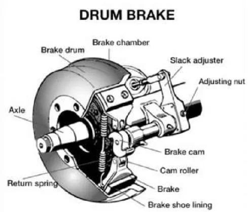
The drum brake is located at each end of the vehicle axles. The braking mechanism is inside the drum, and the wheel is bolted onto the drum. The braking force is transferred from the brake chamber to the brake shoes, where friction is created against the drum. Figure 7 presents each component and its placement in the system

Figure 7 - Schematic illustration of drum brake assembly. [7]

The drum brake itself consists mainly of the drum and the brake shoes, however, the slack adjuster and cam are needed to transfer the forces from the brake chamber to the drum. There are advantages to using a drum brake over other options: they are generally cheap to produce, low maintenance, and they have a self-energizing effect which results in less needed input force. [8]

(22)

2.7.1 Slack adjuster

The slack adjuster plays an important role in the brake system, for the brakes to function properly the distance between the brake shoes and drum need to be close but not touching while the brakes are disengaged. As the brake shoes wear down with use this distance will increase, the slack adjuster’s job is to counteract this wear distance to keep the brakes working at maximum efficiency. [9]

Figure 8 - Slack adjuster force.

The brake chamber provides a linear force into the slack adjuster (𝐹 ), as seen in Figure 8. As the force pushes on the adjuster at a length (𝐿 ), torque is created. As the slack adjuster rotates, the angle which the force is being transferred changes (α). When the pushrod is perpendicular to the slack adjuster maximum force is being transferred. The torque created (𝑇 ) can be explained with the following formula: [10]

(23)

2.7.2 Brake cam

The brake cam is a rotating mechanical piece that transforms rotary motion into linear motion. The brake cam is usually shaped as an “S”, also called S-Cam, to be able to provide force into two linear directions into the brake shoes. This force presses the brake shoes against the drum, which produces friction. As the brake pad wears down the s-cam can rotate further which counteracts the wear, however, the slack does need to be adjusted to keep the brake responsive.

Figure 9 - Brake cam assembly. [11]

In Figure 9, as the chamber pushes on the slack adjuster it provides a torque (𝑇 ) that makes the cam rotate. With this, the effective radius (𝑅 ) changes as the slack adjuster rotates, which causes the force output to change. The force being exerted from the cam (𝐹 ) can be calculated using the following formula:

𝐹 = 𝑇

(24)

2.7.3 Brake shoes

The brake shoes are positioned inside the brake drum. Each drum has a leading and a trailing shoe that convert the linear force from the cam into friction, as seen in Figure 10. The brake shoe carries a brake lining that can either be glued or riveted to the shoe, that is pressed against the drum when the brake is pressed. The friction created between the lining and the drum causes the vehicle to slow down. Heat is also generated from the friction which has an impact on the friction, drum brakes are more prone to overheating due to not being able to dissipate heat as good as a disc brake. Drum brakes are generally preferred on long-haul trucks due to being generally more durable which leads to less downtime for replacements.

Each brake shoe has a mechanical advantage that minimize the effort to actuate the brakes, this is called the brake factor.

Figure 10 – Brake factor forces. [12]

The torque of each shoe (𝑇 , 𝑇 ) can be calculated by multiplying the brake factor with the drum radius (𝑅 ). The brake torque (𝑇 ) generated by the shoes is calculated by adding the leading and trailing torque from following equations: [12]

𝑇 = 𝐹 ∙ 𝜇 ∙ 𝑒

𝑚 − 𝜇 ∙ 𝑛 ∙ 𝑅 (2.14)

𝑇 = 𝐹 ∙ 𝜇 ∙ 𝑒

𝑚 + 𝜇 ∙ 𝑛 ∙ 𝑅 (2.15)

(25)

2.8 Friction

Friction is mostly described as the physical resistance produced between two directly contacting entities moving with unequal motion to one another. It is the most fundamental concern in order to perform the braking process [13]. The frictional properties are described by the dimensionless variable quantity of coefficient of friction (𝜇). The coefficient of friction is depending on internal material properties and external environmental properties. The major internal material property to consider are the adhesiveness of the material, affected by the microstructure and surface tension. Contrarily, some of the main external factors to consider are the humidity- and temperature-conditions of the environment. They consequently provide lubrication or changes the structure of the material [14]. As a result of the many factors governing the coefficient of friction it is generally needed to be determined by tests, rather than through a physical model, for increased reliability.

Through the influence of frictional resistances is the mechanical energy converted into heat [15]. It is as a result not uncommon for the brake systems friction-dependent components to reach hundreds of degrees Celsius after a set of performed braking processes. These components include the brake pads, brake shoes, rotor, and drum. The heat generated is maintained within the materials before dissipating to the environment. The coefficient of friction varies depending on the temperature and material used. Sometimes, the coefficient of friction increases with a slight temperature increase. Over higher temperatures do the coefficient of friction instead tend to decrease. This is due to the effect of brake fade. Brake fade is a decrease in performance as a result of reaching the limit of thermal capacity of the components. The thermal capacity can be explained as the materials ability of maintaining heat. This is greatly related to the volume, shape, and type of material[1]. The tendency in the change of coefficient of friction varies greatly between materials, both before and after brake fade. Generally, a more uniformed value of the tendency is preferred in brake pads, as this results in a homogenous brake performance overall. However, the overall value of coefficient of friction value must also be considered, as a higher value will produce higher braking force.

(26)

2.9 Temperature characteristics

As earlier explained is the heat generated a cause of transformation of the kinetic energy used to propel the vehicle forwards. In the process of braking is the kinetic forces (𝐸 ) converted into heat (𝑄) and work (𝑊) by the brake system in use. The conversion is shown by following expression [16]:

𝑄 − 𝑊 = ∆𝐸 (2.17)

The efficiency of the work to heat ratio produced differs between the two systems of drum brakes and disc brakes considered in this paper. Generally, the efficiency is higher in the disc brake system, while the drum brakes makes up for it with higher produced brake power.

Thermal energy is commonly transferred by three different means. These are conduction, convection, and radiation. In conduction is the thermal energy transferred through the solid medium itself and other solid mediums in direct contact. Convection on the other hand indicate the transfer of energy through a fluid. Radiation, lastly, is the process in which thermal energy is transferred through radiant energy in form of electromagnetic waves [17]. In this paper will only conduction and convection be considered, while radiation is neglected. This is due to the small impact radiation will have on the produced heat in the case of brake system. [16]

During the heat generation process is the produced heat contained within the disc and then diffuses over the volume by conduction. This makes the temperature increase throughout the brake disc and the process can be calculated by following equation:

𝐶 ∙ 𝑚 ∙ 𝑑𝑇

𝑑𝑡 = 𝑄̇ − 𝑄̇ (2.18)

Where the inputs are the thermal capacity (𝐶 ), the mass of the disc (𝑚 ), the temperature change over time , the heat input (𝑄̇ ), the heat output (𝑄̇ ). The heat input is given by the produced brake torque (𝑇 ), angular velocity (𝜔) and the heat partition coefficient between the brake disc and the brake pad (𝜎). The equation of the heat input is the following:

𝑄̇ = 𝜎 ∙ 𝑇 ∙ 𝜔 (2.19)

The heat partition coefficient represents the part of the total thermal energy generated going into the disc, while the rest is distributed to the pads and environment. The heat partition can subsequently be described by the following equation for imperfect contact:

(27)

The thermal effusivity is calculated by:

𝜉 = 𝑘 ∙ 𝜌 ∙ 𝐶 (2.21)

Where the inputs are the thermal conductivity (𝑘), the density (𝜌) and the specific heat constant (𝐶 ) of the material.

The heat output (𝑄̇ ) of the system, is instead controlled by the process of convection. In reality, is the heat output controlled by more processes than convection alone. However, when the vehicle is in movement this is the primary factor and is therefore solely considered in this paper. The process of convection can be described by following equation: [18]

𝑄̇ = ℎ ∙ 𝐴 ∙ ∆𝑇 (2.22)

In which the inputs are the surface area (𝐴 ), and the convective coefficient (ℎ) and the temperature difference (∆𝑇). The convective coefficient (ℎ) varies depending on the flow characteristics of the system. The major impacting factor of the flow is in this case the speed at which the vehicle is travelling. [19]

(28)

Method

3 Method

This report has been introduced with a literature study of the brake system components. Each component had its own study where the main task was identified, the inputs and outputs were determined, and how parts of the component could be modeled with physics. The important factors were determined and acts as a foundation to the simulation model. From the theoretical framework, the method for modeling the tool was chosen. Two methods have been used to create the tool and two have been used to validate the performance of the tool.

3.1 Connection between objectives and method

There are four methods used while developing the tool. Both objectives will be answered with the results of the simulation tool, hence it is important to use the correct method of creating the tool.

Excel is the program chosen to store the component performance data and to act as the master template where the user can choose how the virtual test should be performed. The program chosen to develop the actual tool is called Simulink, which is a powerful block diagram program. This program will read all the test data from excel and then process that data through all the modeled components from the theoretical framework, which eventually leads to an output of brake torque.

The other two methods were used to make the tool accurate and trustworthy. Data driven simulation with a physics base is proven to be the best compromise of accuracy and cost. The validation method is then used to prove the accuracy of the previous method. The four methods are crucial to create an easy to use and accurate model, where each method connects to each other, see Figure 11.

•Component data •Master template

Excel

•Data driven •Physics base

Simulink

_{•Compare to phyiscal tests}

•Is the simulation accurate?

(29)

Method

3.2 Excel

Microsoft Excel is a spreadsheet program, using a grid of cells organized in rows and columns. Each cell contains a single data, for example a text, a numerical value, or a formula. The program is specialized in organizing and performing calculations on data. It can be used to analyze data, calculate statistics, and represent data tables. [20]

3.3 MATLAB & Simulink modeling

MATLAB (Matrix Laboratory) is a programming platform designed for engineers and scientists. It provides an environment where problems and solutions are expressed in mathematical notations. [21]

MATLAB is typically used for:  Math and computation  Algorithm development

 Modeling, simulation, and prototyping  Data analysis, exploration, and visualization  Scientific and engineering graphics

 Application development, including Graphical User Interface building

Simulink is a graphical programming environment based on MATLAB, and it is tightly integrated to the rest of the MATLAB environment. Simulink is a data flow graphical programming tool for modeling, simulating, and analyzing dynamic systems. There is a library with customizable set of blocks that can be used to create the systems. [22] Simulink can be used to create block diagrams of physical systems and algorithms, see Figure 12. Real world variables can be modeled into the system for example, friction, gear slippage and hard stops. Simulink is capable of systematic verification and validation of models, which is used to identify errors in design and code. This can reduce the amount of errors found later in the design process. Simulink can be used throughout an entire project, from creating the requirements, through design, implementation, to testing.[23]

(30)

Method

3.4 Data driven simulation with physics base

A physics-based approach is generally the base of simulation tools. However, these physics-based tools have an inherent problem included, and that is that they tend to deviate from reality with a consistent error. The reason behind this is that there is no governing equation expressing the complete physical impact on an item.

For this reason, integrating data generated from tests into the model proves especially useful. With the use of the data it will guide the physical base towards a considerably more reliable result [24]. The results within the range of the data are especially reliable, whereby an interpolation can generate a good approximation between the measurement points. On the other hand, once acting outside of the ranges of the data the results become unpredictable, thus making extrapolations unreliable [25].

A very classic example of the appliance of data driven, physics-based simulation is when determining the water density based on depth in lakes. Figure 13 below represent this example. The yellow dots in the figure represent the data measurement points, the black line contrarily represent the physics-based prediction and the red and blue line correspond to a mix of the two.[26]

Figure 13 - Water density based on depth of lake. [26]

(31)

Method

3.5 Validation & Reliability

The accuracy of the model needs to be validated to implement the tool into brake development. The tool will be validated in two separate ways, on component level and on a systems level.

Each component in the braking system that has been modeled with component data can be validated against that data. If the output is the same in the virtual test as the component test data, the simulation component works as intended.

The system level test will provide information of how all the modeled components work together and how much accuracy can be achieved against a real-world brake test. In this scenario the accuracy will be lower compared to the component tests. To get the data needed, a truck will need to be outfitted with information collecting sensors and the specific components used in the simulation. The truck will then be put on a dynamometer and run specific brake scenarios, that can be replicated in the tool.

(32)

Implementation of methodologies

4 Implementation of methodologies

The implementation of the methodologies focuses on how each component from the theoretical framework has been modeled, with explanations of the inputs, outputs, and the component data used. The equations from the theoretical framework are reintroduced for simplicity’s sake. The system is the combination of all the modeled components, where each part depends on the previous components outputs. The system is modeled in Simulink, where the variables are chosen through the master excel template and inserted into MATLAB from the component data excel files. Component data graphs do not contain values to protect component details and to uphold the non-disclosure agreements.

4.1 Brake pedal

The pedal is modeled based on component data for pedal mass and pedal leverage ratio. The input from the user has been modeled to fit various braking scenarios. In Figure 14 the brake pedal is pressed and held, while in Figure 15 the brake pedal is pressed and then released. The force is used to calculate the displacement of the pedal, which is used to determine how much pressure is being released.

(33)

4.2 Valves & Tubes

The valves and tubes cause a delay based on many variables. Four main factors were taken into consideration while modeling the tool:

 Wheelbase length  Brake chamber size

 If high flow valves are used  Number of ABS modulators

These four factors have been physically tested in all different configurations, giving a spectrum of delay. Depending on how the user sets up the virtual vehicle, the delay will reflect the chosen setup, see Figure 16.

Figure 16 – Valve and tube configuration.

There is also a fifth factor taken into consideration: if the brake chamber is located in the front or rear of the vehicle. The rear brake will have a greater delay due to the tube length being longer, as can be seen in Figure 17.

(34)

4.3 Brake chamber

The test data provides force output from the chamber depending on the pressure input and the position of the pushrod for each chamber variant, see Figure 18.

Figure 18- Chamber force over stroke.

The chamber model has two inputs: pressure and chamber pushrod position. The pressure is controlled by the pedal displacement, and the position of the pushrod is calculated with Newton’s second law. The model has three input pressures that represent output force at different strokes, whereas in reality, the pressure is also between these values. This results in the output values being interpolated. At zero psi there is a negative force present, this due to the spring force.

As the pressure increases and is fed into the chamber, the pushrod moves, thus changing the output force until the max stroke is reached.

(35)

4.4 Disc brake

4.4.1 Brake caliper

The caliper is modeled to calculate the forces active over the caliper. This is done by combining the effect of the leverage arm, the caliper pistons, and the force input from the chamber. The relation between these effects are expressed by following equation of the force over the caliper (𝐹 ):

𝐹 = 𝐹 ∙ 𝐾 . ∙ 𝑁 (4.1)

The mechanical transmission of the energy does not transfer energy at a perfect rate and energy will inevitably be lost. The effect of energy loss for the caliper can be considered in the joints and the connections between components. A specific example of this would be the leverage arm’s connection to the pistons, where a sliding effect between the two is present. Furthermore, there are several mechanical components in the caliper transferring the forces. The resulting energy losses in the subsystem should therefore not be overlooked. To compensate for the energy losses the simulation tool will consider a value for the caliper efficiency (𝐸 ). This results in the total caliper force (𝐹 , ) to be calculated by:

𝐹 , = 𝐹 ∙ 𝐸 (4.2)

The value of the efficiency is in the model assumed to 98% and positioned in the later part of the system to cover the entire caliper.

4.4.2 Leverage arm

The leverage arm is integrated in two separate ways in the disc brake part of the simulation. One data driven approach, that is utilizing data received from physical tests to express the mechanical advantage ratio, and a second, purely physics-based approach. The two scenarios are used separately throughout the model.

For the first variant, the change in the mechanical advantage ratio is interpreted through a graph. The graph expresses the relationship between the change in ratio to the stroke movement in mm and it is given by the component test data of the caliper. The graph is therefore data driven, and it can be seen in Figure 20. The data is then used to produce a data map and integrated into the model. With the integration of the data map is the total forces over the caliper (𝐹 , ) calculated. Due to the high reliability of this

(36)

Figure 20 - Mechanical advantage ratio characteristics as it changes over stroke length.

As for the second variant of determining the leverage arm ratio, a trigonometrical mathematical expression has been derived for application through a physics-based approach. This is done by considering the displacement of the push rod and the resulting angle changes in the leverage arm. The mechanical advantage ratio (𝐾𝐿𝑒𝑣. 𝑎𝑟𝑚) can be

described by following equation with complementary Figure 21:

𝐾 . =

𝐿 ∙ cos 𝛽

𝐷 (4.3)

Figure 21 - Leverage arm movement for physics-based approach.

Where the inputs used are the length of the leverage arm (𝐿 ), the angle of the leverage arm (𝛽) and lastly, the distance to the piston center from leverage arm pivot-point (𝐷 ). The values of the lengths of and between the components are in this case only assumed values. Also, in this specific expression is the eccentric bearing not considered, and the pivot point is therefore constant. Realistically, the pivot-point would change depending on the stroke received.

(37)

4.4.3 Piston

The expression of the leverage arm ratio can further be incorporated into trigonometrical expressions showing the relationship of the stroke length (Δ𝑋) to the piston displacement (Δ𝑌). There will be two mathematical expressions or scenarios needed to cover the full movement cycle. The first scenario covers the movement of the displacement in Figure 22, which shows the event of the angle of the leverage arm (β), ranging from 0° to 90°.

The movement of the displacement for the second scenario is covered in Figure 23. This scenario instead covers the event of the angle of the leverage arm (β) being negative and ranging from -90° to 0°.

The piston displacement (Δ𝑌) can for scenario one be described according to following expression:

Δ𝑌 = ∆𝑋 cos 𝛼

𝐿 ∙ cos 𝛽

𝐷

(4.4)

Figure 22 - Describing figure of the variables used to calculate piston displacement, 0° < 𝛽 < 90°.

Figure 23 - Describing figure of the variables used to calculate piston displacement, −90° < 𝛽 < 0°.

(38)

For scenario 2 the piston displacement is (Δ𝑌) described according to the following expression:

Δ𝑌 = ∆𝑋 ∙ cos 𝛼

𝐿 ∙ cos 𝛽

𝐷

+ tan 𝛽𝜊 ∙ 𝐷 _(4.5)

With the initial angle of the leverage arm (𝛽𝜊).

Furthermore, in order to model the component in Simulink is an additional expression needed. This expression covers the relationship between the two dynamic input variables of the stroke (Δ𝑋) and the leverage arm angle (𝛽) and can be seen below:

ΔX = 𝐿 (sin 𝛽 − sin 𝛽)

𝐶𝑜𝑠 𝛼 (4.6)

Through solving the equation for the leverage arm angle (𝛽), the equation becomes:

𝛽 = 𝑠𝑖𝑛 sin 𝛽 − cos 𝛼 ∙ ΔX

𝐿 (4.7)

The piston displacement function is thereafter used to calculate the spring force active at the piston position. This is to correctly simulate the return of the piston to its neutral position when the brakes are released. The spring force will therefore be included into the total brake force of the system, in which it is subtracted from the force over the caliper, acting onto one of the pistons.

(39)

4.4.4 Brake pad

A friction map can be created for use in the brake pad modeling based on component test data. This data map covers the effective friction change depending on the temperature in the model. The friction characteristics can be seen in Figure 24.

Figure 24– Friction change over temperature for brake pad.

With the friction map it is possible to calculate the resulting brake force (𝐹 ) in the model with following equation:

𝐹 = 2 ∙ 𝐹 , ∙ 𝜇 (4.8)

The brake force (𝐹 ) is perpendicular to the total caliper force (𝐹 , ) and

acting opposite the wheel movement. Due to the friction being temperature dependent, a temperature model is required. With the temperature model is the data map then integrated to give the correct friction change of the pads. The temperature modeling will be explained as a separate part in the chapter.

4.4.5 Rotor

The last component in the brake disc system is the rotor. This component will be modeled in the model by a purely physics-based approach. The idea behind modeling this component is to calculate the produced brake torque (𝑇 ) by the air disc brake system. To calculate the brake torque, the effective radius needs to be considered. The effective radius (𝑅 ) is the length of the lever action used in the calculation and is modeled using following equation:

𝑅 = 𝑅 − 𝑂 − 𝑊

2

(4.9) Where the inputs are the radius of the rotor (𝑅 ), the outer distance between the rotor and the brake pad (𝑂 ) and lastly, the full width of the brake pad (𝑊 ). With this it is possible to determine the brake torque active during a brake action in an air disc brake system by using following equation:

(40)

4.5 Drum brake

4.5.1 Slack adjuster

The slack adjuster is modeled entirely from a physics approach, where the torque output varies depending on the angle of the slack arm. However, the component has two static component data inputs, the slack arm length and initial mounting angle.

𝑇 = 𝐹 ∙ 𝑆𝑖𝑛(α) ∙ 𝐿 (4.11)

There are two dynamic inputs to the slack adjuster model, the chamber force (𝐹 ) and effective angle of the slack adjuster (α). These values will change depending on the previous components output. This results in a dynamic output of torque (𝑇 ) created from the slack adjuster.

4.5.2 Brake cam

The cam model is dependent on the angle of the slack arm. As the pushrod changes the angle of the slack adjuster, the effective radius of the cam will change. This radius is data driven depending on the effective angle, see Figure 25.

Figure 25– Cam radius change over effective angle.

𝐹 = 𝑇

𝑅 (4.12)

The other output from the slack adjuster model, slack torque (𝑇 ), is then divided by the dynamic radius (𝑅 ) to get the linear force that is transferred to the brake shoes (𝐹 ).

(41)

4.5.3 Brake shoes

The brake factor has three dynamic values and four static inputs. The slack arm torque, cam radius, friction coefficient and shoe temperature are all dynamic values and will change over time. The static inputs are all length variables that can be different depending on the drum that is being used, but once defined they do not change.

𝑇 = 𝐹 ∙ 𝜇 ∙ 𝑒

𝑚 − 𝜇 ∙ 𝑛 ∙ 𝑅 (4.13)

𝑇 = 𝐹 ∙ 𝜇 ∙ 𝑒

𝑚 + 𝜇 ∙ 𝑛 ∙ 𝑅 (4.14)

The torque provided by the slack adjuster is experienced in the CAM which rotates to exert the force (𝐹 ). This force is transferred to the brake shoes where the brake factor acts as a lever arm that applies friction against the drum. These forces are multiplied with the drum radius (𝑅 ) to get brake torque of each shoe.

As the brake shoes provide friction on the drum, the vehicle slows down. The friction coefficient is dependent on the temperature of the drum, this temperature will increase if the vehicle is moving and braking simultaneously. Depending on the temperature of the drum, the friction coefficient will be different, as can be seen in Figure 26. The optimum temperature that provides the most amount of friction to the drum will be above ambient but less than its maximum operation temperature. This means that the friction will increase as the vehicle starts to brake, then the friction will decrease after the temperature reaches a certain threshold.

(42)

4.6 Temperature modeling

The temperature model uses a basic tire model and vehicle model in order to simulate the wheel- and vehicle-dynamics during braking, which affects the temperature build up. The velocity (𝑣) can through division of the tire radius (𝑅 ) also be expressed in angular velocity (𝜔). In the case of this model is the tire radius assumed. The relationship for angular velocity is expressed by the following:

𝜔 = 𝑣

𝑅 (4.15)

With the angular velocity and through using the equations explained in the theoretical framework, is the heat generation calculated. The calculation of heat generation uses the produced brake torque (𝑇 ), heat partition coefficient (𝜎) and angular velocity (𝜔) as inputs. The heat generation of the system can be expressed with:

𝑄̇ = 𝜎 ∙ 𝑇 ∙ 𝜔 (4.16)

Only assumed values for the heat partition is in this case modeled.

Following step of the temperature modeling involve modeling the heat dissipation of the system. The heat dissipation is limited to convection of the system, whereby the surface area (𝐴 ) and initial temperature (𝑇 ) are assumed. With the initial temperature and the calculated temperature (𝑇) is the temperature difference (∆𝑇) generated. As for the convection coefficient (ℎ), is it instead interpreted from a graph of how it changes over velocity in air as shown in Figure 27. This is then converted into a data map and integrated into the model. The relation between the inputs for convection are the following:

𝑄̇ = ℎ ∙ 𝐴 ∙ ∆𝑇 (4.17)

Figure 27 - Convective coefficient change over vehicle velocity.

(43)

Whereby it is then solved for the temperature. The temperature change is given over the time through the equation and is therefore needed to be integrated so that the temperature can be modeled at specific points. The solved equation is finally expressed by the following:

𝑇 = 𝑄̇ − 𝑄̇

𝐶 ∙ 𝑚 (4.19)

With the final temperature modeled it is now possible to be combined with the changing friction coefficient explained for both brake pads and brake shoes.

(44)

Analysis

5 Analysis

This chapter analyses the strengths, weaknesses, and accuracy of the tool. To make the tool usable for brake development, the limits and inaccuracies need to be known. Each component has been modeled differently and various variables have simplified or in some parts even excluded. The analysis also considers how the system reflects reality on a component scale and a system scale.

5.1 Data driven

Each component modeled using a data driven approach reflect reality with a high confidence level. However, if the component test data has low frequency of measurements the model has to interpolate values which results in small inaccuracies. An example of this is the brake chamber model which has data for three pressure inputs that gives different force outputs. In reality the pressure is also between these three data values. In the model the maximum pressure, zero pressure, and a middle value is measured. In the brake chamber specifically, it is important to cover the extreme values (max, zero). These values are important due to covering the produced pressure when the brake pedal is fully displaced and at resting position. Further input values could be measured for each brake chamber, but it would be costly for a marginal increase in accuracy.

5.2 Physics base

The use of a physics-based approach will always have a consistent error compared to measurements, however, replacing all the physics models would take excessive testing for diminishing returns. One of the variables that have not been incorporated to the physics model is the friction between the components. There will always be a loss of power when a force is transferred to another component. This results in the model having inaccuracies during power transfer.

5.3 Valves & Tubes

The valves and tubes component have potential to be modeled in a more accurate way. The delay caused from the air reservoir to the brake chamber is difficult to predict and is detrimental to know for the brake system to be within the regulations. A separate simulation could be created where it takes into account the friction, turbulence, tube length, tube diameter, temperature, chamber size and number of valves. Due to the system using pneumatic air, the flow can change greatly depending on each variable, and if the air reaches high enough flow the fluid density can change. The valves and tubes model reflects reality due to measurements, but the configuration freedom is quite low. The user can choose four different options for the model which creates 16 unique delays for each axle. The tool lacks configurability in tube placement, which a lot of time is dedicated to testing today.

(45)

Analysis

5.4 Temperature modeling

The model for heat generation in the system has room for an upgrade. The temperature determines the friction force output of the system and is therefore an important consideration. As of right now these consists of only basic temperature applications of convection and conduction. The material properties in the model may be based on realistic values, though these are only for a specific material. By incorporating these variables with the master excel sheet system used for the other data driven components, with validated component values, the reliability will increase. Even easily produced variable inputs such as brake rotor and pad surface area are assumed. Simply incorporating the actual values for these will significantly increase the reliability. As mentioned, the model currently only consists of basic applications of convection and conduction. As a result, some of the additional heat generation and heat dissipation effects present in the process are instead excluded in this paper. As such, the temperature module could use an upgrade. This can be done in more ways than one. The temperature is currently maintained by the components producing the frictional resistance, alone. Realistically the temperature would be continuously transferred to other components in direct contact by means of conduction. This to average out the temperature. Other components can thus be included into the conduction process to improve accuracy.

Similarly, convection is the sole heat dissipation process active in the system. This is due to it providing the main heat dissipation when the vehicle is in movement [18]. However, this is not the case when the braking process instead brings the vehicle to a full stop. In the case of a vehicle in full standstill, the processes of radiation and conduction will be more prominent for the cooling process. This scenario can be simulated in the tool and should hence also be incorporated.

Furthermore, the temperature model is identically modeled for both the disc and drum brake. This is obviously wrong, as explained in earlier occasions, the heat dissipation properties are worse for the drum brakes. This is due to the closed off system of the drum brake better containing heat, as well as the disc brakes being actively designed for better heat dissipation. This should be taken into consideration when running the simulation tool in its current state.

5.5 Test validation

To validate the accuracy of the model, the results have been compared to an old truck dynamometer test. The specific components that were used on the truck were not fully specified, which means that the results will differ from the simulation model. The specific brake case could be replicated, as in, how much force was applied to the pedal over a set time. Comparing the model with the physical testing showed that the tool was around 85% accurate. It is difficult to determine if the uncertainty of used components gave a stronger accuracy or weaker accuracy. Considering that most components use data that reflect how the part works in real life, the model was expected to have a high accuracy. Each component that uses component test data has high confidence, due to the output being based on measurements. These data driven components are valid, but full system tests need to be performed to validate the entire tool and to get a more precise understanding of how accurate the model is.

(46)

Results & Discussion

6 Results & Discussion

The results and discussion chapter will provide the results of the problem statements; “How can simulations of brake systems be used to reduce development cost and time?” and “How is the virtual vehicle built for rapid testing?”.

6.1 How can simulations of brake systems be used to reduce

development cost and time?

There are many benefits for using the virtual vehicle simulation over physical testing. If a decision needs to be made quickly, a test can be performed in one minute if the component data is available, as opposed to around 14 days for a physical test. If you incorporate acquiring data for components and the time it takes to analyze the simulation results, a decision can be taken in less than one third of the average time it currently does.

Figure 28 - Simulink block model.

One of the strongest reasons that the tool is useful for brake development is that the tool is highly customizable, each part can be replaced with another from the database. This gives the tool a high range of uses, where each component of the simulation can be measured in the simulation, see Figure 28.

Due to the nature of a simulation, no resources need to be spent while performing the test. Physical testing requires huge investments, for example, a truck will be allocated to the test and someone must spend hours setting up and performing the test. With a virtual vehicle a spectrum of different vehicle setups can be tested, with different components and different braking scenarios, all in a shorter time and with minimal resources spent.

When a supplier releases a new component, it must be delivered, mounted, and then a test must be done to gather data if the new component performance is worth the investment. With a virtual vehicle the engineer can request the data needed from the

(47)

Results & Discussion

6.2 How is the virtual vehicle built for rapid testing?

The tool is customizable through a master excel sheet, where the user enters the part numbers of the components. The tool reads the excel sheet, finds the data that is linked to each part number, and then runs the simulation.

Figure 29 – Master excel template.

The virtual vehicle can be configured with different components and in different scenarios. This makes the tool usable in a variety of situations, where the user can choose the speed of the vehicle, its mass, driver brake tendencies and specific components used in the truck, as can be seen in Figure 29.

If the data is not available for a current component or if a brand-new component needs to be tested if the investment is worth the upgrade, a template can be sent to a supplier to be filled in. Once the data is acquired, the user can run the part number in the master excel.

The person using the tool does not need to know how to write MATLAB code or how to adjust the Simulink model. Currently all the user must do is plug in the part numbers then navigate to the result graph of a component or the entire system in the program. However, the master excel could be improved with an output field, where the user could specify what component graph is wanted to get an automatic output window.