http://www.diva-portal.org
Postprint
This is the accepted version of a paper published in Finite elements in analysis and design (Print). This
paper has been peer-reviewed but does not include the final publisher proof-corrections or journal
pagination.
Citation for the original published paper (version of record):
Hansbo, P., Rashid, A., Salomonsson, K. (2016)
Least-squares stabilized augmented Lagrangian multiplier method for elastic contact.
Finite elements in analysis and design (Print)
http://dx.doi.org/10.1016/j.finel.2016.03.005
Access to the published version may require subscription.
N.B. When citing this work, cite the original published paper.
Permanent link to this version:
Least–squares stabilized augmented Lagrangian
multiplier method for elastic contact
Peter Hansbo, Asim Rashid, Kent Salomonsson
Department of Mechanical Engineering, Jönköping University, SE–55111 Jönköping, Sweden
Abstract
In this paper, we propose a stabilized augmented Lagrange multiplier method for the finite element solution of small deformation elastic contact problems. We limit ourselves to friction–free contact with a rigid obstacle, but the formulation is readily extendable to more complex situations.
Key words: Lagrange multiplier, stabilization, contact, augmented Lagrangian
1. Introduction
This paper is motivated by the recent work by Chouly and Hild [9] on Nitsche’s method for contact problems. In their work, the contact conditions were incorpo-rated into the bilinear form to transform the variational inequality describing the contact problem to a nonlinear variational equality. We here point out that the same can be done for a more standard stabilized Lagrange multiplier method if we aug-ment the Lagrangian using the standard approach of, e.g., Alart and Curnier [1]. Us-ing a multiplier method has an advantage compared to the Nitsche method in that there is an increased freedom in choosing the multiplier space. For example, using a continuous multiplier with nodes coinciding with the displacement nodes on the surface we can use nodal quadrature schemes to emulate point Lagrange multipli-ers (at least for low order elements). For such schemes, contact will be checked at the nodes as is usually done in engineering practice. This is not possible following the Nitsche approach.
A basic issue when using Lagrange multipliers to enforce contact is the num-ber of degrees of freedom in the discrete Lagrange multiplier space. If too many constraints are used, the discrete system might be singular, and if there are too few constraints, there might be unphysical violation of the non-penetration condition. There are, basically, two different possibilities to obtain a stable discretization. The first approach is to choose discrete spaces that fulfill the inf–sup condition which guarantees stability (cf. [7]). A well-known example of such a scheme is the mor-tar method introduced by Bernardi, Maday, and Patera [5], and applied to contact problems by Ben Belgacem, Hild, and Laborde [4]. The other option is to change the bilinear form in such a way that stability is ensured, as pioneered by Barbosa
and Hughes [2, 3] and this is the approach taken in this paper. We consider an aug-mented version of the stabilized Lagrange multiplier method introduced by Hansbo, Lovadina, Perugia, and Sangalli [11] and adapted to contact by Heintz and Hansbo [12]. Unlike the method in [11, 12], which was based on a global polynomial approx-imation of the multiplier, the method herein is suitable for locally defined multipli-ers.
The rest of the paper is organized as follows. First, we describe the proposed method. Secondly, we make some comments on the stability and convergence prop-erties of the discretization. Finally, we present some numerical results and conclu-sions.
2. Problem formulation
We consider an elastic body covering the domainΩ in Rd, d = 2,3, with bound-aryΓ = ΓD∪ ΓN∪ ΓCand outward pointing normal n. We consider the case where the domains are subjected to proper Dirichlet (onΓD) and traction (onΓN) bound-ary conditions and are coming into frictionless contact alongΓC, and are subjected to volume forces f ∈ (L2(Ω))d. The unilateral contact problem in linear elasticity
consists in finding the displacement field u satisfying the equations and conditions
−∇ · σ = f inΩ, σ = 2µε(u) + λ∇ · uI inΩ, u = 0 onΓD, σ · n = 0 onΓN, un≤ 0, σn(u) ≤ 0, unσn(u) = 0 onΓC, (1)
withσn(u) := n ·σ(u)·n, un:= u ·n, and with ε(u) the strain tensor with components
ε(u) =1
2¡∇ ⊗ u + (∇ ⊗ u)
T¢ ,
where (w ⊗ v)i j= wivj, withµ =2(1+ν)E andλ =(1+ν)(1−2ν)νE , where E is the modulus
of elasticity,ν is Poisson’s ratio, and with I the identity tensor. We shall assume that µ and λ are constant in the domain.
2.1. An augmented Lagrangian method
One interesting way of deriving an augmented Lagrangian method is to replace σn(u) by a Lagrange multiplier p (the contact pressure) so that the final line in (1) is
written
un≤ 0, p ≤ 0, unp = 0, (2)
(the Kuhn–Tucker conditions) and, using the notation, [a]+:=
½
a if a > 0,
0 if a ≤ 0, (3)
replace conditions (2) by the equivalent statement p = −1
withγ a positive number, cf . Chouly and Hild [9, Prop. 2.1]. Defining function spaces
V = {v ∈ (H1)d: v = 0 on ΓD}, Q = L2(ΓC), (5)
and seeking (u, p) ∈ V ×Q we have by Green’s theorem, with a(u, v ) := Z Ωσ(u) : ε(v)dΩ, L(v) := Z Ωf · v dΩ, that a(u, v ) − Z ΓCp vn ds = L(v)
where v ∈ V and vn:= v · n. Following [9] we write vn= vn+ γq − γq for an arbitrary
function q ∈ Q, so that we may write a(u, v ) −
Z
ΓCp (vn− γq) ds −
Z
ΓCγp q ds = L(v).
Replacing the p in the first integral by the expression in (4) we finally obtain the problem of finding (u, p) ∈ V ×Q such that
a(u, v ) + Z ΓC 1 γ[un− γp]+(vn− γq) ds − Z ΓCγp q ds = L(v) ∀(v,q) ∈ V ×Q. (6)
This problem is related to seeking stationary points to the functional Π(u,p) := a(u,u) − L(u) +
Z ΓC 1 2γ£un− γp ¤2 +ds − Z ΓC γ 2p 2ds, (7)
which is the well known nonlinear variational equality version of the augmented La-grangian method, see, e.g., Alart and Curnier [1]. While replacing the standard vari-ational inequality formulation (cf., e.g., [4, 13]) by a nonlinear varivari-ational equality is not strictly necessary in an augmented method, cf. Chen [8], the nonlinear equality approach is well suited for applying Newton methods, and allows for avoiding the activation/deactivation of multipliers as the contact zone changes during nonlinear iterations. In a standard variational inequality setting, an active set of multipliers is typically used, which favours iterative algorithms able to accomodate active sets, cf. [6].
The formulation (7) constitutes the starting point for our finite element approx-imation. A remarkable fact is that by replacing p byσn(u) in (7) we formally obtain
the Nitsche method of [9] which can be interpreted as a stablilized multiplier method in the linear case [15]. The augmented Lagrange multiplier method is, however, not a stabilized method and is subject to the standard problems of matching spaces for stability of the discrete problem, cf. [7].
3. Finite element methods
Assume that we are given a triangulationThof the domainΩ. We denote by h the meshsize ofTh. We introduce the finite element space
~
Vh= {v : v ∈£H1(Ω
i)
¤d
where P1(K ) denotes the space of affine polynomials on K . OnΓCwe introduce a family of spaces Qhof discrete multipliers. As a particular case, we will consider the spaces Qhi, i = 0 or i = 1, of piecewise constants or linears defined as follows: the interfaceΓCis decomposed as the union of the faces of the triangulationThonΓC which gives a set of facesFChconsisting of the faces of simplices inTh.
Our particular choices of multiplier space are
Qh0= {q ∈ Q : q|K∈ P0(K ), ∀K ∈ FCh}, (8)
and
Q1h= {q ∈ C0(ΓC) : q|K∈ P1(K ), ∀K ∈ FCh}, (9)
and finite element methods based on (6) are to find (uh, ph) ∈ ~Vh×Qhi such that a(uh, v ) + Z ΓC 1 γ h uhn− γphi +vnds = (f , v) ∀v ∈ ~V h, (10) and Z ΓC µ 1 γ h uhn− γphi ++ p h¶ q ds = 0, ∀q ∈ Qhi. (11)
These methods are not in general stable, so we proceed to add a stabilizing term. 3.1. Least-squares stabilization
The difficulty in choosing approriate combinations of discrete spaces for the fi-nite element approximation (10)–(11), in particular with respect to stability of the discrete system, prompts the introduction of a stabilized discrete functional whose stationary point are sought:
ΠStab(uh, ph) := Π(uh, ph) − Z ΓC δ 2(p h − σn(uh))2ds. (12)
This approach is close to that introduced in [12] and analyzed by Hild and Renard [13], but different in being an augmented Lagrangian method. Another recent re-lated contribution can be found in Tur et al. [16].
Introducing Bh(u, p; v , q) := a(u, v) + Z ΓC 1 γ£un− γp ¤ +(vn− γq) ds − Z ΓCγpq ds − Z ΓCδ¡p − σn(u)¢ ¡q − σn(v )¢ ds, (13)
the stationarity ofΠStableads to the problems of seeking (uh, ph) ∈ ~Vh×Qhi such that
Bh(uh, ph; v , q) = L(v) ∀(v, q) ∈ ~Vh×Qhi. (14) Here we make the particular choices
γ := h/γ0, δ := h/γ1,
whereγ1is a number to be chosen so as to ensure stability of the discrete system
4. A brief comment on the source of stability
We shall here briefly comment on the source of the stability of the method and the significance for the choice ofγ0. Let us for simplicity assume there is contact all
alongΓCand consider the resulting matrix problem arising from (14): · S B BT −C ¸ · u p ¸ = · f 0 ¸ , (15)
which, if we use a basisϕi for the displacements and a basisψi for the multipliers,
is constructed as (S)i j= a(ϕj,ϕi) + 1 γ Z ΓCn · ϕjn · ϕid s − δ Z ΓCσn(ϕj)σn(ϕi) d s, (B)i j= − Z ΓCn · ϕjψid s − δ Z ΓCσn(ϕj)ψid s (C)i j= δ Z ΓCψjψid s. We split S = S1− δS2, where (S1)i j= a(ϕj,ϕi) + 1 γ Z ΓCn · ϕjn · ϕid s.
For stability, it is then sufficient to have, for arbitrary v 6= 0,
vT(S1− δS2) v ≥ c1|v|2
and, for arbitrary q 6= 0,
qT¡BTS−1B + C¢ q ≥ c 2|q|2
for constants c1and c2, i.e., that both S and BTS−1B+C are positive definite matrices.
As is well known (cf., e.g., [9]),
CIuTS1u > h uTS2u (16)
where h is the meshsize and CI depends on the elastic moduli but not on h (this
argument works elementwise as well). This means that ifδ < h/CI, or, equivalently, γ1> CI, the matrix S is positive definite. The determination of CIcan be performed
by a local eigenvalue problem and it is tabulated for some different approximations in [10]. This in turn means that BTS−1B—while in worst case singular—certainly is
positive; since C is positive definite we conclude that BTS−1B+C is also positive
def-inite, as desired. Thus, one might say that this stabilization method borrows some excess stability from S1in order to create stability for the multipliers.
-0.2 0 0.2 0.4 0.6 0.8 1 1.2 -0.2 0 0.2 0.4 0.6 0.8 1 0.12 0.14 0.16 0.18 0.2 0.22 0.24 0.26 -0.06 -0.04 -0.02 0 0.02 0.04
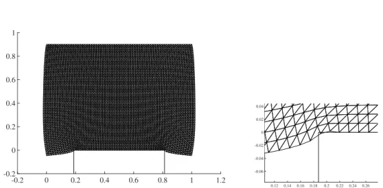
Figure 1: Displacements using the unstabilized scheme.
5. Numerical examples
5.1. Stability enhancement
We begin by showing the effect of the stabilization method. The example we con-sider is non–smooth with an elastic object covering the domain (0, 1) × (0,1) being pushed downwards using the Dirichlet boundary condition u = (0,−0.1) at y = 1. The body comes in contact with a rigid foundation that stretches from x = 0.1875 to x = 0.8125. We set E = 100, ν = 0.3 and γ0= 200. For the approximation of the
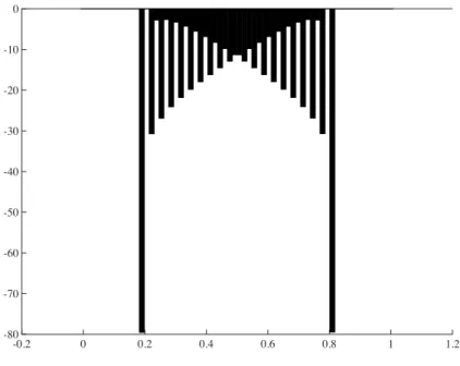
contact pressure we use Qh0 and we takeΓCto be the line y = 0. We compare the casesδ = 0 (no stabilization) with δ = h/200 (stabilized). In Fig. 1 we show the dis-placement field and a blow up at the corner of the foundation for the unstabilized scheme. The displacement field exhibits no serious signs of instability, whereas the contact pressure, shown in Fig. 2 exhibits strong oscillations.
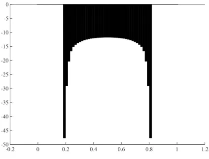
The corresponding results for the stabilized scheme are shown in Figs. 3–4 and we note that the oscillations in the contact pressure is alleviated and the displace-ment field has a monotone variation near the singularities.
5.2. Herzian contact
In this section we solve the Hertzian problem of an elastic cylinder contacting a rigid surface by using the method presented in previous sections. We assume small deformations and frictionless contact. The numerical results will also be compared to an analytical solution. A distributed load is applied on the top boundary edge of the half cylinder as shown in figure 5a.
The distribution of the normal tractionσndue to applied load W =R wd s, where w is load per unit length, can be determined analytically by the following relation which is based on the Hertzian contact theory [14]
-0.2 0 0.2 0.4 0.6 0.8 1 1.2 -80 -70 -60 -50 -40 -30 -20 -10 0
Figure 2: Contact pressure using the unstabilized scheme.
-0.2 0 0.2 0.4 0.6 0.8 1 1.2 -0.2 0 0.2 0.4 0.6 0.8 0.12 0.14 0.16 0.18 0.2 0.22 0.24 0.26 0.28 -0.04 -0.02 0 0.02 0.04 0.06
-0.2 0 0.2 0.4 0.6 0.8 1 1.2 -50 -45 -40 -35 -30 -25 -20 -15 -10 -5 0
Figure 4: Contact pressure using the stabilized scheme.
x y
w
(a) Cylinder loading
-1 -0.8 -0.6 -0.4 -0.2 0 0.2 0.4 0.6 0.8 1 -0.4 -0.2 0 0.2 0.4 0.6 0.8 1 (b) Mesh refinement Figure 5: The elastic half cylinder contacting the rigid planar surface.
σn(x) = σmaxn r 1 −³x b ´2 , (17)
where x is the distance from the symmetry line of the cylinder, b is the width of the contact zone given as
b = 2 s
W R(1 − ν2)
πE , (18)
andσmaxn is the maximum normal traction given as
σmax
n =
s W E
πR(1 − ν2). (19)
Here R is the radius of the cylinder,ν is the Poisson’s ratio and E is the modulus of elasticity. For the results presented in this work, the parameters are set as follows: R = 1, E = 7000,ν = 0.3 and w = 100. For the finite element analysis, plane strain assumption is adapted and movement of a point at (0,1) is fixed along x-axis . The movement of the rigid surface is fixed both in x and y. The cylinder is finely meshed in the area which could come in contact with rigid surface as shown in figure 5b. The outer edges of all the elements in this area are set to have equal length. A contact zone is defined on the surface of the cylinder within the limits −0.25 < x < 0.25. The number of active multipliers is determined in advance and do not change during the iterations.
The root-mean-square error (RMSE), defined as s µ Z ΓC ³ σana n − σ aug n ´2 d s ¶ (20) whereσanan is the analytical normal traction computed by (17) and
σaug n = 1 γ h unh− γphi +,
will be used to compare the results. The length of the boundary edge, he, of a
con-tacting element will be used to describe the meshing of cylinder.
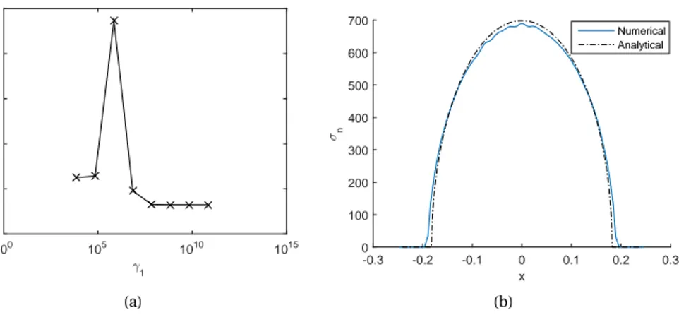
In figure 6a the error is shown as a function ofγ1whenγ0= E and he= 0.01.
It can be seen that after the initial jump, the error shows decreasing trend asγ1
in-creases. The minimum error occurs whenγ1= E × 107. Figure 6b shows the
distri-bution of the normal traction when the error is minimum.
In figure 7 the error is plotted against two measures of mesh size, hav and he,
whenγ1= E ×107andγ0= E. The average element size, havis defined as hav=pA(Ω) Nel
where A(Ω) is the area of the domain and Nelis the number of elements. Quadratic
convergence can be observed in figure 7a.
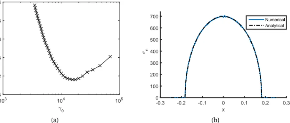
In figure 8a the error is plotted againstγ0whenγ1= E × 107 and he = 0.001.
The minimum error occurs whenγ0= E/0.45. Figure 8b shows the distribution of
100 105 1010 1015 error 0 20 40 60 80 100 .1 (a) x -0.3 -0.2 -0.1 0 0.1 0.2 0.3 <n 0 100 200 300 400 500 600 700 Numerical Analytical (b)
Figure 6: (a) Error as a function ofγ1, whenγ0= E and he= 0.01. (b) Distribution of normal traction
when error is minimum
log 10(hav) -1.8 -1.7 -1.6 -1.5 -1.4 log 10 (error) 0.2 0.4 0.6 0.8 1 1.2 1.4 (a) hav log 10(he) -3 -2.8 -2.6 -2.4 -2.2 -2 -1.8 -1.6 log 10 (error) 0.2 0.4 0.6 0.8 1 1.2 1.4 (b) he
. 0 103 104 105 error 1.5 2 2.5 3 3.5 4 (a) x -0.3 -0.2 -0.1 0 0.1 0.2 0.3 <n 0 100 200 300 400 500 600 700 800 . 0=E/0.45, /0=E x 1e+07 Numerical Analytical (b)
Figure 8: (a) Error as a function ofγ0, whenγ1= E × 107and he= 0.001. (b) Distribution of normal
traction when error is minimum
6. Conclusions
In this paper, a stabilized augmented Lagrange multiplier method for the finite element solution of elastic contact problems is presented. Results from two numeri-cal examples are also presented. In the first example it has been shown that stability of the method depends on theγ1. In the second example, the Hertzian problem is
solved and compared to an analytical solution. It also investigates the dependence of error onγ0,γ1and mesh size. In the future this method could be extended to
contact between two elastic bodies with friction and large deformations.
References
[1] Alart, P., Curnier, A., 1991. A mixed formulation for frictional contact problems prone to Newton like solution methods. Comput. Methods Appl. Mech. Engrg. 92 (3), 353–375.
[2] Barbosa, H. J. C., Hughes, T. J. R., 1991. The finite element method with La-grange multipliers on the boundary: circumventing the Babuška-Brezzi condi-tion. Comput. Methods Appl. Mech. Engrg. 85 (1), 109–128.
[3] Barbosa, H. J. C., Hughes, T. J. R., 1992. Boundary Lagrange multipliers in finite element methods: error analysis in natural norms. Numer. Math. 62 (1), 1–15. [4] Ben Belgacem, F., Hild, P., Laborde, P., 1999. Extension of the mortar finite
el-ement method to a variational inequality modeling unilateral contact. Math. Models Methods Appl. Sci. 9 (2), 287–303.
[5] Bernardi, C., Maday, Y., Patera, A. T., 1994. A new nonconforming approach to domain decomposition: the mortar element method. In: Nonlinear partial differential equations and their applications. Collège de France Seminar, Vol. XI (Paris, 1989–1991). Vol. 299 of Pitman Res. Notes Math. Ser. Longman Sci. Tech., Harlow, pp. 13–51.
[6] Bertsekas, D. P., 1982. Constrained optimization and Lagrange multiplier meth-ods. Academic Press, New York-London.
[7] Brezzi, F., Fortin, M., 1991. Mixed and hybrid finite element methods. Vol. 15 of Springer Series in Computational Mathematics. Springer-Verlag, New York. [8] Chen, Z., 2001. On the augmented Lagrangian approach to Signorini elastic
contact problem. Numer. Math. 88 (4), 641–659.
[9] Chouly, F., Hild, P., 2013. A Nitsche-based method for unilateral contact prob-lems: numerical analysis. SIAM J. Numer. Anal. 51 (2), 1295–1307.
[10] Hansbo, P., Larson, M. G., 2002. Discontinuous Galerkin methods for incom-pressible and nearly incomincom-pressible elasticity by Nitsche’s method. Comput. Methods Appl. Mech. Engrg. 191 (17-18), 1895–1908.
[11] Hansbo, P., Lovadina, C., Perugia, I., Sangalli, G., 2005. A Lagrange multiplier method for the finite element solution of elliptic interface problems using non-matching meshes. Numer. Math. 100 (1), 91–115.
[12] Heintz, P., Hansbo, P., 2006. Stabilized Lagrange multiplier methods for bilateral elastic contact with friction. Comput. Methods Appl. Mech. Engrg. 195 (33-36), 4323–4333.
[13] Hild, P., Renard, Y., 2010. A stabilized Lagrange multiplier method for the fi-nite element approximation of contact problems in elastostatics. Numer. Math. 115 (1), 101–129.
[14] Popov, V., 2010. Contact mechanics and friction: Physical principles and appli-cations. Springer-Verlag Berlin Heidelberg.
[15] Stenberg, R., 1995. On some techniques for approximating boundary condi-tions in the finite element method. J. Comput. Appl. Math. 63 (1-3), 139–148. [16] Tur, M., Albelda, J., Navarro-Jimenez, J. M., Rodenas, J. J., 2015. A modified
per-turbed Lagrangian formulation for contact problems. Comput. Mech. 55 (4), 737–754.