BULLETIN NO
STOCKHOLM 2000
ISRN KTH-BYT/R—2000/180-SE
ISSN 0346-5918
180
Division of
BUILDING TECHNOLOGY
Department of Building Sciences
Kungl Tekniska Högskolan
The ORC Method – Effective Modelling of
Thermal Performance of Multilayer Building
Components.
Jan Akander
~
ϑ
0~
q
0~
ϑ
n~
q
nDoctoral Dissertation
Stockholm 2000
Dept. of Building Sciences Div. of Building Technology
The ORC Method – Effective Modelling of Thermal
Performance of Multilayer Building Components
Jan Akander
Akademisk avhandling
Som med tillstånd av Kungliga Tekniska Högskolan i Stockholm framlägges
till offentlig granskning för avläggande av teknologie doktorsexamen den
8:mars 2000 kl 14:00 i sal L1, Drottning Kristinas väg 30, Stockholm.
Avhandlingen försvaras på engelska.
Fakultetsopponent:Professor Joe A. Clarke, University of Strathclyde
Huvudhandledare: Professor Guðni Jóhannesson, KTH
ISSN 0346-5918, ISRN KTH-BYT/--00/180-SE
Stockholm 2000
The ORC Method – Effective Modelling of Thermal Performance of Multilayer
Building Components
Jan Akander
Div. of Building Technology
Dept. of Building Sciences
Kungliga Tekniska Högskolan
SE – 100 44 Stockholm
Abstract
The ORC Method (Optimised RC-networks) provides a means of modelling one- or
multidimensional heat transfer in building components, in this context within building
simulation environments. The methodology is shown, primarily applied to heat transfer in
multilayer building components. For multilayer building components, the analytical
thermal performance is known, given layer thickness and material properties. The aim of
the ORC Method is to optimise the values of the thermal resistances and heat capacities
of an RC-model such as to give model performance a good agreement with the analytical
performance, for a wide range of frequencies. The optimisation procedure is made in the
frequency domain, where the over-all deviation between model and analytical frequency
response, in terms of admittance and dynamic transmittance, is minimised. It is shown
that ORC’s are effective in terms of accuracy and computational time in comparison to
finite difference models when used in building simulations, in this case with IDA/ICE.
An ORC configuration of five mass nodes has been found to model building components
in Nordic countries well, within the application of thermal comfort and energy
requirement simulations.
Simple RC-networks, such as the surface heat capacity and the simple R-C-configuration
are not appropriate for detailed building simulation. However, these can be used as basis
for defining the effective heat capacity of a building component. An approximate method
is suggested on how to determine the effective heat capacity without the use of complex
numbers. This entity can be calculated on basis of layer thickness and material properties
with the help of two time constants. The approximate method can give inaccuracies
corresponding to 20%.
In-situ measurements have been carried out in an experimental building with the purpose
of establishing the effective heat capacity of external building components that are
subjected to normal thermal conditions. The auxiliary wall method was practised and the
building was subjected to excitation with radiators. In a comparison, there were
discrepancies between analytical and measured effective heat capacities. It was found that
high-frequency discrepancies were to a large extent caused by the heat flux sensors.
Low-frequency discrepancies are explained by the fact that the exterior climate contained other
frequencies than those assumed in the interior climate.
Key words : Building component, building simulation, heat transfer, thermal
Dept. of Building Sciences Div. of Building Technology
The ORC Method – Effective Modelling of Thermal
Performance of Multilayer Building Components
Doctoral Dissertation
Jan Akander
Stockholm 2000-02-06
ISRN KTH-BYT/R-2000/180-SE
ISSN 0346-5918
Doctoral Dissertation ISRN KTH-BYT/R-2000/180-SE
ISSN 0346-5918
PREFACE
I would like to thank Professor Guðni Jóhannesson for initiation of the projects, for constructive guidance through these projects and for the trust he has given me on coming forth with results within the projects. I am him indebt for introducing me to the fascinating field of frequency response with application to building physics. Also, the help and fruitful discussions with my colleagues at the Department of Building Sciences are warmly appreciated. A special gratitude is directed to PhD. Guofeng Mao, for assisting within the field of dynamic multi-dimensional heat transfer calculations and heat transfer in general, and to Christer Hägglund for practical advice on experimental matters. A thanks is also put forth to my co-authors Dr Asima Norén, Associate Prof. Engelbrekt Isfält and Prof. Ove Söderström. I happened to stumble into that project during a coffee break - is this when business actually is done...? A blessing is extended to Ms. Ninni Bodin, who kept track of all my paperwork.
A sincere gratitude is directed to Hans Persson, Maj Persson and Bill Hermansson at AB Svensk Leca for their co-operation within the Röskär project. Their curiosity, wise ideas and patient understanding is acknowledged.
The fellows at Brisdata AB are not forgotten. The useful ideas, positive criticism and software related issues from Axel Bring and Per Sahlin are well appreciated. I wish Mika Voulle at HUT, Finland, continued success in component library modelling. Keep up the good work!
I wish Håkan Rodin at Flooré AB all future success on electrical and water borne floor heating systems. It started with a project on measurements of a radiant floor in 1992...
Last but not least, I would like to thank the support and understanding that my wife Ulrika and energy bundles (my children) Sara and Sebastian have shown during the darkest and sunnier moments in times of research.
The grants from the Swedish Council for Building Research (BFR) and AB Svensk Leca are gratefully acknowledged.
Jan Akander Stockholm, Feb 2000
TABLE OF CONTENTS
1
SCOPE
7
2
A BRIEF OVERVIEW OF THIS THESIS
9
3
BACKGROUND
12
4
THERMAL FREQUENCY RESPONSE
13
4.1 The thermal performance of multilayer building components 13
4.1.1 The frequency domain solution of the heat conduction equation 13
4.1.2 Admittance and dynamic transmittance 15
4.1.3 Informative asymptotes of admittance 15
4.1.4 The Bode Diagram 16
4.1.5 Switching frequencies 18
5
EFFECTIVE HEAT CAPACITY
19
5.1 Measurement of the effective heat capacity 20
5.1.1 The measurement method 22
5.1.2 The boundary conditions 22
5.1.3 Measured results in comparison with analytical results 23
5.1.4 Reasons for deviation in analytical and experimental results 25
5.2 The approximate method 26
5.3 EN832 - A calculation method that makes use of the effective heat capacity 28
6
THERMAL MODELS
30
6.1 The heat transfer matrix of serially connected thermal resistances and heat capacities 30
6.2 Finite difference method 30
6.2.1 Modelling the response of the semi-infinite solid 31
6.3 The ORC Method 33
6.3.1 Model deviation procedure 33
6.3.2 Optimisation of RC-networks 34
6.3.3 Fields of application: State-of-the-art and future perspectives 38
1 Scope
This thesis focuses to a large extent on thermal frequency response of multilayer building components. The work is therefore relevant to thermal performance of building components; how thermal
performance can be characterised, how thermal performance can be modelled and experimentally be validated. The target reader group is therefore scientists within the research field of heat transfer in buildings.
Within the scope of this thesis, the thermal performance of multilayer components is characterised with applications in the Bode diagram, which is a well-know way of putting forth transfer functions. In this application, the Bode diagram is used to analyse the thermal performance of multilayer building
components, in terms of what type of response is obtained for various frequencies of thermal processes. The frequency response can be that of a semi-infinite solid, or that of a simple mass or it can be purely resistive. The admittance procedure and dynamic transmittance (Danter 1973, Milbank and Harrington-Lynn 1974) are key issues within this context. Attention is focused at which frequencies a change in these types of responses occur on basis of material layer properties and layer order within building components. These frequencies are here called switching frequencies.
An informative quantification of frequency response is the entity called effective heat capacity. Actually, this term is widely accepted and used, though the definition is not clearly defined. A
discussion is put forth on the use of two models that serve as a basis for the definition, on the choice of boundary conditions, and within what context this term will or may be used. Pros and cons for the use of one of the two models are stated from a physical point of view and also from a more practical sense. In-situ measurements have been performed on various building components as to experimentally validate this entity, where measurement methodology and data treatment are important factors that influence the final results.
Moreover, the frequency domain analysis can be used to study the performance of thermal models that are composed of chains of thermal resistances and heat capacities, such as those of finite difference methods and RC-networks. For a given building component, the analytical thermal performance can be calculated with frequency domain solution of the heat conduction equation. The thermal performance of the model can be evaluated against the analytical performance within the frequency domain. An
implication of this is therefore to optimise the thermal model with respect to model inaccuracy, boundary conditions and thermal processes within the simulated system. This is conveniently done by means of optimised RC-networks (ORC’s) that represent multilayer building components. The ORC method is used for optimising the parameters of an RC-network within the frequency domain. When the agreement between analytical and model performance can be considered to be adequate, the ORC can be used in time domain simulations, such as building simulation programs. Modelling and results from the building simulation program IDA/ICE are shown, where a comparison is made when building components are modelled with finite differences or with ORC’s. ORC’s are convenient for modelling multidimensional heat transfer, such as dynamic heat flow through thermal bridges and ground heat loss (Mao 1997).
Special attention has been given to a set of proposed drafts and accepted standards within building physics. Since the results of calculation procedures of these standards are dependent on building component types - much due to climatic circumstances and national building traditions - it is necessary to test and validate these codes with application on national factors. Also, it is necessary to review the background theory and definitions within the standards, as to check that these conform to the state-of-the-art of the field of application. Parts of three standards are frequently referred to in one way or another within this thesis. These are:
• prEN ISO 13786: 1998 E. Thermal Performance of Building Components - Dynamic thermal characteristics - Calculation methods. CEN/TC 89/WG 4/N176, Brussels.
• EN 832 (1998). Thermal performance of buildings Calculation of energy use for heating -Residential buildings. European Committee for Standardisation (CEN), Brussels.
• EN ISO 13370 (1998). Thermal performance of buildings – Heat transfer via the ground – Calculation methods. European Committee for Standardisation (CEN), Brussels
It should be noted that the aim of this thesis is not to validate these standards. Comparisons are made since this work and these standards have common fields of application, unless the standards have directly been used to provide numerical results.
The thesis summarises the six papers that are included as appendices. Consequently, the aim of this first part is to highlight important issues presented in these six papers, to underline conclusions and to tie up ”loose ends” between the papers. To a minor extent, some issues may be re-discussed as to give another viewpoint.
2 A brief overview of this thesis
This thesis is a summary of six papers that are enclosed. These papers primarily evolve the applications of one of the most fundamental equations within building physics, namely Fourier’s equation for heat conduction in solids. The work made here is to a large degree based on the application of the frequency domain solution on multilayer building components, especially on the characterisation and the
modelling of building component thermal performance. This field is by no means new, but it is indeed significant and necessary as reflected in a proposal to European (EN) and international (ISO) standard with the title ”Thermal Performance of Building Components”. For this reason, a series of articles have been produced with the title ”Thermal Performance of Multilayer Building Components”. This series is composed of totally four papers and are inserted in the end of this thesis under the chapters called Paper 1 to 4. Yet, each paper has been written so that it can be read as a stand-alone paper. Two additional papers with applications on heat transfer are included.
The title of this thesis, “The ORC Method – Effective Modelling of Thermal Performance of Multilayer Building Components”, has the intention of summing up the contents of this thesis with respect to the methodology used for determining one (or multidimensional) heat transfer in building components. The analytical frequency domain solution of the heat conduction equation provides the “true” thermal performance of the building component. This thermal performance can be modelled, in the frequency and in the time domain, by means of RC-networks. When the parameters of an RC-network are
determined as to give the model a thermal performance that agrees well with the analytical performance, for a wide range of frequencies, the outcome is an optimised RC-network (ORC). RC-networks are chains of thermal resistances and heat capacities (i.e. lumped parameter models) that can comprise a single heat capacity, for example an effective heat capacity, to more complex configurations, such the 5-node ORC configuration as illustrated on the cover.
The first paper (Paper 1) within the series, “The Thermal Performance of Multilayer Components -Applications of the Bode Diagram” contains fundamentals on the methodology used and serves as a platform for the other papers within the series. More specifically, the entities thermal admittance and dynamic transmittance are stated. These heat transfer functions, which are thermal performance characteristics of a building component, are conveniently displayed in the Bode diagram. The Bode diagram is widely used for example within automation and control theory. Within the current application, it serves as a visual aid as it reveals if the response of a building component is that of a simple mass, a pure thermal resistance or the semi-infinite solid. Switch frequencies quantify when there is a change in thermal performance. The Bode diagram also visualises asymptotes of admittance. This is penetrated to a greater extent in the second paper, but within the scope of the first paper, asymptotes and switching frequencies can be used for discretisation of cell size of a finite difference model applied to a building component. Model and analytical performance can be plotted in the Bode diagram, to be directly compared. This provides background theory to the fourth paper, where the optimised RC-network method (ORC) is introduced.
The second paper within the series (Paper 2) deals with the effective heat capacity of multilayer building components and is closely related to the proposed EN ISO standard on dynamic thermal performance of building components, prEN ISO 13786 (1998). In this paper, a discussion is put forth on what and how the effective heat capacity of a building component can be defined and determined. The main content of the paper is a proposal of a new method on determining the effective heat capacity by means of real numbers only: the material layer thermal properties and thickness. The ”correct” (analytical) value involves calculations using real and imaginary numbers. The new method can be used as a complement to the present normative method of Annex A of prEN ISO 13786, since the method gives more reliable results than the proposed standard. The method gives an inaccuracy that in general is less than 20%.
The aim of the third paper is to validate effective heat capacity procedures experimentally (Paper 3 with the sub-title “Experimental Assessment of the Effective Heat Capacity”). Measurements were performed with the auxiliary wall method. The heating system of an experimental building was subjected to a Pseudo Random Binary Sequence (PRBS) to excite building components. The thermal response of various building components was recorded. Monitored data was transformed into the frequency domain
with Fast Fourier Transform (FFT), for calculation of the measured effective heat capacity. A comparison between theoretical and measured results shows adequate agreement. The paper also focuses on sources of experimental errors and shows that the choice of boundary conditions in the definition of effective heat capacity has a large influence on the result.
The fourth and last paper within the series concerns the optimisation of RC-networks as to give equivalent thermal performance as multilayer components. Having been stated in the first paper, the method for comparing model and analytical performance is essential in the optimisation procedure. The optimisation procedure involves minimising model performance deviation for a wide range of
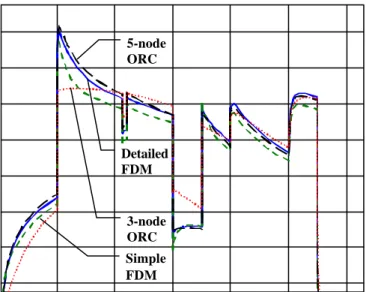
frequencies. Various RC-network configurations are shown, as well as their fields of application. Again, the definition of the effective heat capacity is discussed, since this entity is based on the configuration of a simple RC- (or C-) network. This paper also shows differences in ORC performance as opposed to the performance of a conventional finite difference model within the building simulation program IDA/ICE. Results of an ORC with five mass nodes give good agreement with results from a detailed finite difference model, but the ORC requires less computational time. A discussion is also put forth on the subject of modelling multidimensional heat transfer with ORCs. These are very efficient for this purpose and the method has been practised (Akander et al 1996, Mao 1997), but this application is beyond the scope of this thesis.
Papers 5 and 6 are beyond the scope of the series entitled ”The Thermal Performance of Multilayer Building Components”. However, Paper 5, with the title ”The Effect of Thermal Inertia on Energy Requirement in a Swedish Building – Results Obtained with Three Calculation Models”, is closely related to this series. This paper shows by means of simulations that the thermal inertia of a building has an influence on energy requirement of a multifamily building situated in a northern climate. Whereas two co-authors of the paper used detailed building simulation programs (TSBI3 and BRIS), the author of this thesis utilised the calculation procedure of European Standard EN832 (at the time it was a proposed standard). The simplified calculation procedures of prEN832, that makes use of the effective heat capacity of a building, gave results that agreed well with results of far more detailed simulation program TSBI3. A special note should be made at this stage: the proposed effective heat capacity procedure, that was a part of prEN832, that was at the time of working defined differently than at present.
Paper 6 is more or less miscellaneous within the frame of this dissertation. Having the title ”Reducing Ground Loss from a Heated Underfloor Space – A Numerical Steady-state Case Study”, this work is limited to steady-state calculations, focusing on heat loss from a heated underfloor space. The aim of that work was to reduce heat loss and system temperatures without affecting heat delivered to the living space, nor the building method for erecting the house. A comparison was made between results from models in two- and three dimensional heat transfer as well as calculated U-values from applications in EN ISO 13370 (1998). The agreement between 2-D and 3-D numerical models was very good. The U-value for a slab-on-ground according to the EN-ISO calculation procedure was considerably lower than for the numerical models. An EN-ISO equation was modified as to give the U-value of the heat
transmittance from a heated underfloor space. The modified equation gave reliable results. As measurements and calculations on air infiltration in the underfloor space were conducted, the paper concluded that infiltrating air should be included in the heat balance of the underfloor space.
At the time that this doctoral dissertation was sent for publication, the status of the papers were:
PAPER 1: Submitted to Nordic Journal of Building Physics.
Akander J. and Jóhanneson G. The Thermal Performance of Multi-Layer Components - Applications of the Bode Diagram.
PAPER 2: Submitted to Nordic Journal of Building Physics.
Akander J. The Thermal Performance of Multilayer Building Components - A Method for Approximating the Effective Heat Capacity.
Akander J. The Thermal Performance of Building Components – Experimental Assessment of the Effective Heat Capacity.
PAPER 4: Submitted to Nordic Journal of Building Physics and revised
Akander J. The Thermal Performance of Building Components – The Methodology of ORC and Applications.
PAPER 5: Published in International Journal of Low Energy and Sustainable Buildings.
Norén A., Akander J., Isfält E. and Söderström O. (1999). The Effect of Thermal Inertia on Energy Requirement in a Swedish Building – Results Obtained with Three Calculation Models . International Journal of Low Energy and Sustainable Buildings, Vol 1 . Available at http://www.bim.kth.se/leas
3 Background
This thesis is a documentation of some of the results obtained from primarily two major projects. The first is ”Energiflöden i byggnadskomponenter - beräkningsmetoder - simuleringar”, which resulted in the licentiate thesis ”Efficient Modelling of Energy Flow in Building Components - Parts 1 and 2 ”
(Akander 1995). To a large extent, the work focused on the modelling of multilayer building components by means of optimised RC-networks (ORC’s). The outcome was implemented within the building simulation program IDA/ICE. This did not mean that the development of optimisation procedures ended at the time when the project was officially terminated. Further development is summarised within this thesis.
The second project bears the name ”Två småhus på Röskär” (in English: ”Two residential houses at Röskär”). The so-called Röskär project was to allow the erection of experimental buildings by industrial companies and thereby to have special technical building solutions theoretically and experimentally analysed. This was the role of the Division of Building Technology within the Department of Building Sciences at KTH. Despite the depression within the Swedish national economy during the early and mid-nineties, which hit hard on the building sector, two experimental buildings were erected. One was the IEA house, which was built by the division and financed by the Swedish Council of Building Research. AB Svensk Leca built the other house. The main objective of the first stage of the project was to study the influence of heat capacity on energy requirement. For this reason and also due to that the division under the leadership of Professor Gudni Jóhannesson has a tradition of using frequency response analysis as method to tackle heat transfer problems, the effective heat capacity played an important role within the project. At the same time, Sweden is subject to a set of new European
standards, whereof two as a matter of fact involve the so-called effective heat capacity. In one of these, which currently is a draft, the effective heat capacity is defined (prEN ISO 13786:1998 E. Thermal Performance of Building Components - Dynamic thermal characteristics - Calculation methods.). The other is a calculation method for determining the energy requirement of a residential building, EN 832 (1998), that makes use of the effective heat capacity when the thermal inertia of the building is taken into account. The Röskär project was therefore a golden opportunity for investigating the role of heat capacity on energy requirement, to review what the term effective heat capacity means and how it may be defined and measured, what results can be expected and how these are to be interpreted and used. The project has also lead to a communication and information exchange between the university and industrial parties, with industrial application of results. More general information on the Röskär project can be found in (Johannesson 1994) and (Akander and Jóhannesson 1997).
4 Thermal frequency response
Thermal frequency response is a central issue within this thesis. Reasons for analysing thermal behaviour in terms of frequency response are the following.
• There is a frequency domain solution to the Fourier’s heat conduction equation if the considered system is linear. This means that analytical analysis can be made on thermal performance.
• Thermal performance can be characterised by using the definition of admittance and dynamic thermal transmittance, which are frequency dependent transfer functions.
• The effective heat capacity can be defined and calculated on basis of admittance.
• Thermal models composed of chains of thermal resistances and heat capacities, such as finite difference and RC-network models, can be optimised within the frequency domain as to give desired model accuracy. Model performance deviation can be determined since the analytical performance is known. By means of the ω-RC transform, these models can be used in time domain simulation programs.
• Multidimensional heat transfer in building components can be modelled with simple one- or
multidimensional RC-networks. The multidimensional heat transfer of the building component can be modelled by means of finite difference programs that determine admittance and dynamic
transmittance of various surfaces. This thermal performance can be modelled with simplified equivalent RC-networks. This point is beyond the scope of this paper, but is nevertheless a strong reason.
• Theory can experimentally be validated, even though a mathematical transformation of time domain data into the frequency domain (or vice-versa) is necessary.
A mandatory criterion that has to be fulfilled in frequency domain calculations is that the system is linear. In this thesis, it is mainly multilayer plane building components that are studied. If the building component is to be linear, all material properties and layer thickness have to be constant. For a linear system, each frequency component of a variable can be superposed. If the thermal entities in question are density of heat flow (heat flux) q and temperature θ at the two surfaces, these can be represented as the sum of the steady state component and the sum of each frequency component, or mathematically formulated such that
∑
∞ = + = 1 ~ j j q q q (1a) and∑
∞ = + = 1 ~ j j θ θ θ (1b)Here, qand θ depict the steady state component (i.e. the mean value of a long time series). The terms j
q~ and θj ~
represent heat flux and temperature oscillation for one frequency. If the considered series is time limited, ∞ is substituted by an integer.
4.1 The thermal performance of multilayer building components
4.1.1 The frequency domain solution of the heat conduction equation
This thesis evolves around the solution of one equation. This equation is the heat conduction equation that was originally stated by Fourier. The equation, without a heat source term, is for heat transfer in one dimension expressed as
t x a ∂ ∂ = ∂ ∂ θ θ 2 2 (2)
Here, a is thermal diffusivity of the material, x space co-ordinate and t time.
Various scientists have derived a frequency domain solution to the heat conduction equation. Some use the penetration depth of a heat wave, such as Claesson et al (1984) and also prEN ISO 13786 (1998). The set of equations used here were as formulated by Carslaw and Jaeger (1959). A heat transfer matrix of a sinusoidally excited slab was defined such that
= 0 0 1 1 1 1 n n q D C B A q ~ ~ ~ ~ θ θ (3)
Sinusoidal surface heat flux (density of heat flow rate) and surface temperature oscillations are denoted by q~ and θ~. These are functions of one angular frequency ω, here depicted by the superscript ”∼”. Surface 0 is the excited surface, whereas surface n is the obverse surface that is subject to different boundary conditions discussed later. The heat transfer matrix contains complex elements, here
( )
(
k l i)
A1=cosh ⋅ 1+ (4a)( )
(
)
( )
i k i l k B1 ⋅ + + ⋅ − = 1 1 sinh λ (4b)( )
i(
k l( )
i)
k C1 =−λ⋅ 1+ ⋅sinh ⋅ 1+ (4c)( )
(
k l i)
D1=cosh ⋅ 1+ (4d) with a k ⋅ = 2 ω and c a ⋅ = ρ λ (4e)The determinant of the heat transfer matrix of a plane component is always unity.
For a multilayer component, the heat transfer matrix of the component is the product of the heat transfer matrix of each material layer. The matrix multiplication result in a 2x2 heat transfer matrix
= = 0 0 0 0 1 1 1 1 2 2 2 2 3 3 3 3 n n q D C B A q D C B A D C B A D C B A q ~ ~ ~ ~ ~ ~ θ θ θ (5)
The theory assumes that the system is linear. Each frequency component can be treated separately. Input values give oscillations of heat flux or temperature with the same frequency.
λ
ρ
c
0θ
~
0q~
nθ
~
nq
~
ll admittance transmittance
Figure 1: To the left: Material parameters, temperature oscillation and heat flux direction for a homogeneous slab. To the right: Illustration of admittance and transmittance (see section 4.1.2).
4.1.2 Admittance and dynamic transmittance
The admittance procedure, introduced by Danter (1973) and Milbank and Harrington-Lynn (1974), is a way of defining frequency response of a building component. Admittance is the quotient of heat flux and temperature oscillation at one surface of the component, thus having the unit W/(m2⋅K). Admittance has direction, and is defined positive on leaving the component via the surface, see figure 1.
0 0 0 q Y θ~ ~ − = (6)
Admittance is influenced by the boundary condition at the other surfaces. Here, applied to a multilayer building component, the admittance of surface 0 is such that
B A Y0 =
(
θn =0)
~ (7a) D C Y0 =(
q~n =0)
(7b) B A Y0 = −1(
θ~n =θ~0)
(7c)Dynamic transmittance depicts heat flow at surface n due to a temperature oscillation at surface 0. Dynamic transmittance is the same in both directions, differing only by a minus sign.
0 n D q T θ~ ~ = (8)
The definition gives that
B TD
1
=
(
θ~n =0)
(9)This section is in more detailed described in Paper 1, including references to related work by other authors.
4.1.3 Informative asymptotes of admittance
When the value of angular frequency ω can be considered to be high or low, admittance converges to a certain value, see the appendix of Paper 2. For a high frequency thermal process, the value of admittance approaches
( )
i c Y0 =− 1⋅ 1⋅ 1⋅ 1+ 2 ω ρ λ (10)This is the response of the semi-infinite solid, where the magnitude is λ1⋅ρ1⋅c1⋅ω W/(m 2⋅
K) and phase shift -135°. The value is independent of the boundary condition at surface n.
If the considered thermal process takes place at a node that is coupled to the surface of a building component by means of a thermal surface resistance, R for example, admittance converges to thesi value
si i
R
Y =− 1 (11)
Here, the index i represents an internal node, such as a representative indoor air node.
If the thermal process is of a low frequency nature, the response will be boundary condition dependent, and in the case of multilayer components also influenced by material layer order. The asymptotic values for a homogeneous slab are such that
R Y0 ≈−1
(
θn =0)
~ (12a) l c i Y0 ≈−ω⋅ρ⋅ ⋅(
q~n =0)
(12b) 2 0 l c i Y ≈−ωρ⋅ ⋅(
θ~n =θ~0)
(12c)4.1.4 The Bode Diagram
The Bode diagram is commonly used within the field of automation and control systems for illustration of transfer functions in general (Åström 1968). Since admittance and dynamic transmittance are frequency-dependent transfer functions, the Bode diagram is suitable within this application as originally used by Jóhannesson (1981).
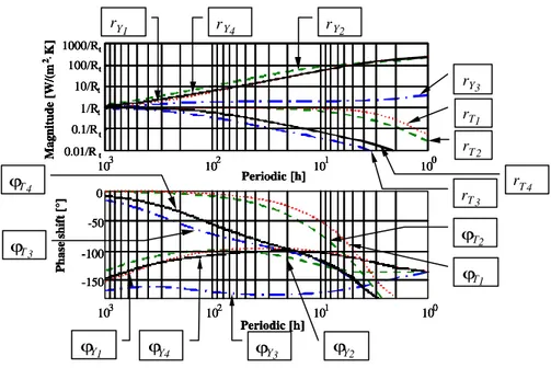
The Bode diagram plots magnitude and phase shift as function of frequency, though frequency has been converted to time period as this eases legibility. A general layout of the diagram is shown in figure 2. The upper diagram shows magnitude and the lower phase shift. Attention should be given to the upper diagram, where the lines with constant values are displayed. These ”constant” values can be compared with the asymptotic values of admittance (equations 10, 11 and 12a-c). On starting with the y-axis, thermal performance of resistive nature are plotted as horizontal lines, drawn in relation to the inverse of the thermal resistance of the building component, R .t
100 101 102 103 M a g n it u d e [ W /( m 2*K ] Periodic [h] -150 -100 -50 0 P h a s e s h if t [° ] Periodic [h] 100 101 102 103 1000/Rt 100/Rt 10/Rt 1/Rt 0.1/Rt 0.01/Rt ω⋅χt ω⋅χt/10 ω⋅χt/100 ω⋅χt/1000 10 b ω 100 b ω ω b
Figure 2: The upper diagram illustrates magnitude as function of periodicity. The y-axis, thus the horizontal lines, shows the response of a thermal resistance, with R being the total thermalt resistance of the building component. The filled slanted lines show the response of a simple mass
(ω⋅χt), whereas the dotted lines represent the thermal response of the semi-infinite solid (b ω ). The lower diagram shows phase shift for the three types of response as stated above.
Next, there are four lines with the slope 1:1, which depict the thermal performance of a simple mass, or as formulated in the figure, a function of angular frequency times a value corresponding to a heat capacity, here denoted by C . Three lines that do not go below the t 1Rt -level show the thermal response of the
semi-infinite solid. These are parallel with the line b ω , where b is the thermal effusivity of a material and is defined as
c
b= λ⋅ρ⋅ (13)
Phase shift is more easily interpreted. The phase shift of the semi-infinite solid is –135°, it is –90° for the simple mass and –180° for a pure thermal resistance.
An example from Appendix 1 is shown below, more can be found in Appendix 1, 3 and 4. The thermal performance of the exemplified wall of table 1 is plotted in figure 3. Here, the thermal performance is based on the assumed boundary condition θ~n =0.
Table 1: Material data for a roof. The innermost layer is listed first.
Material d [m] λ [W/(m⋅K)] ρ [kg/m3] c [J/(kg⋅K)] R [(m2⋅K)/W] χ [J/(m2⋅K)]
Concrete 0.040 1.2 2400 880 0.0333 84480
Mineral wool 0.120 0.04 200 750 3.0000 18000
Roofing felt 0.004 0.26 1100 1500 0.0154 6600
Three distinct types of admittance performances (stages 1 to 3) can be seen. Stage 1 is the range of periodicity where the thermal performance can roughly be regarded to be resistive. The dashed line depicts the asymptotic performance of a pure thermal resistance. Stage two is when the thermal performance of the component is said to have the performance of a simple mass. The asymptote (the dashed line) has values from the equation −iω⋅χconcrete, where χconcrete is the heat capacity of the concrete layer. In this case, the agreement between analytical response and the asymptote is good, and as seen, this provides a basis for what is called the “effective heat capacity” of a building component (see the following sections). The last range, stage 3, is when the response is that of the semi-infinite solid. Here, the thermal effusivity is that of the concrete layer. The periodicity ranges of the three types of responses can be estimated by means of switching frequencies, which are described in the next section. 100 101 102 103 M a g n it u d e [ W /( m 2*K ] Periodic [h] -150 -100 -50 0 P h a s e s h if t [° ] Periodic [h] 100 101 102 103 1000/Rt 100/Rt 10/Rt 1/Rt 0.1/Rt 0.01/Rt ω⋅χconcrete ω concrete b
Stage 1 Stage 2 Stage 3
Admittance
Transmittance
Transmittance
Figure 3: The Bode diagram of the building component as listed in table 1, with the boundary condition θ~n =0. Magnitude and phase shift is plotted (filled curves) for admittance and
transmittance. Three ranges of periodicity are marked (stages 1 to 3) depending on response type, as well as admittance asymptotes (dashed lines) within each range.
The response of a building component is dependent on the choice of boundary conditions. This will not explicitly be shown within this context as this issue is more thoroughly discussed in Paper 1.
4.1.5 Switching frequencies
Switching frequencies are useful for determining at what periodicity there is a change in response (thermal behaviour). In the current example, switching frequencies separate the three different stages.
Starting with stage 2, the response is virtually that of a simple mass, valid for a periodicity Tbetween 3600
2 3600
2π⋅R1⋅χ1 ≤T ≤ π⋅Rt⋅χ1 (15)
In this example, χ was large, being 77% of the total heat capacity 1 χ . Therefore, a transient region ist found at stage 3, where this region is approximately
3600 2
3600
2π⋅Rt⋅χ1 ≤T ≤ π⋅Rt⋅χt (16)
The response of the building component is that of the semi-solid for periodicity that is faster than
3600 2π⋅ 1⋅χ1
≤ R
5 Effective heat capacity
The term effective heat capacity is actually a quantification that corresponds to the part of the total heat capacity of a building component that participates in dynamic heat exchange between the component and the environment. It is therefore natural to base the definition of effective heat capacity on
admittance, as noted earlier in the applications of the Bode diagram. However, in order to complete the definition, a model has to be set up. Jóhannesson (1981) studied two models to determine what he called the ”active heat capacity”. The models are the surface heat capacity and the heat capacity of the RC-configuration (network) as displayed in figure 4. These two models have also appeared in various draft versions of prEN ISO 13786 with the title ”Thermal performance of building components- Dynamic thermal characteristics - Calculation methods”. The most recent versions use the latter model. Paper 2 deals to some extent on how the definition of effective heat capacity should be formulated. The following issues must be considered when the definition of the effective heat capacity is formulated.
~
θ
0~
q
c χc rc Rθ
~
c~
q
c~
q
r~
θ
0χ
Figure 4: To the left: The surface heat capacity model. To the right: The RC-configuration model.
The surface heat capacity model has an admittance that mathematically is a pure imaginary number, whereas admittance is composed of a real and a complex number. However, on taking the absolute value of the analytical (Y ) and model admittance, the magnitudes can be set equal such that0
ω χ Y0
c = (18)
The surface heat capacity can model magnitude of admittance for building components that have the response of a simple mass very well. It does not model phase shift well, since the value is constantly -90º. Building components that have the response of the semi-infinite solid can only be modelled at the frequency for which the effective heat capacity is calculated from. Examples are found in figures 2 and 4 of paper 4.
The RC-configuration model has an admittance that is composed of a real and an imaginary number. For a given frequency, the values of the thermal components within the model are determined such that
− = 0 1 Re Y R ; ⋅ = 0 1 Im 1 Y rc ω χ (19)
Analytical magnitude and phase shift is modelled exactly for the given frequency. Magnitude and phase shift is better modelled for a wider range of frequencies than the surface heat capacity model. However, the semi-infinite solid is again not well modelled, other than for the calculation frequency. This model consistently results in larger values than the surface heat capacity, as shown below in table 2.
A main issue is to determine what the results for such calculations are to be used for. In terms of product specifications, dynamic entities are welcome, such as the effective heat capacity and the decrement factor. The U-value is of course the most important entity that describes thermal
performance. The effective heat capacity and the decrement factor are complements to the U-value, and the question is if these two values, that are based on the 24-hour periodic, are enough to give the entire thermal performance of a building component. For simulations, these entities are practically insufficient,
as pointed out by Kre (1993): these merely ”illuminate otherwise analysed principles”. The analytical equations 4 to 5 and the principle of superposition can be used for this purpose and give more reliable results. Therefore, the effective heat capacity is primarily an entity that describes how much heat can be stored within a building component, and secondarily an entity that describes when the storing takes place (this can only be done in combination with a thermal resistance). Hence, the RC-configuration gives the redundant value of the thermal resistance, and the value of the effective heat capacity will at the same time be meaningless if it does not interact with the resistance. These values are alone not comprehensive. Also, the modelled phase shift is redundant in practical calculations at this level of detail. For these purposes, the surface heat capacity is more comprehensive and practical to use.
So far, nothing has been mentioned about what boundary conditions should be assumed within the calculations. The three boundary conditions that may be used are that θ~n =0, q~n =0 and θ~n =θ~0. On using asymptotic admittance values of equations 10 and 12a-c, the calculated heat capacities receive values as expressed in table 2. Note that the boundary condition θ~n =0 is inconvenient. The effective heat capacity interprets the setting of constant temperature at surface n as being done by an infinite mass when frequency approaches zero. The boundary condition θ~n =θ~0 is preferred among these options, as is the condition of the EN ISO standard proposal. However, the influence of the phase shift of θ~n θ~0 has a large influence on the effective heat capacity, as will be shown in section 5.1.2 (from Paper 3). Table 2 also lists differences in results from the two models. The value of χ may exceedRC
C
χ by a factor ranging from 1 to 2 .
Table 2: The values of effective heat capacities χ and C χ for a slab. These are boundaryRC condition dependent. The values of χ may be larger values than RC χ , as seen on the right handC side. Heat capacity as ω→0s-1 C χ χRC Heat capacity as ∞ → ω s-1 C χ χRC 0 ~ = n θ ∞ ∞ θ~n =0 λρc ω 2λρc ω 0 ~ = n q χt χt q~n =0 λρc ω 2λρc ω 0 n θ θ~ =~ χt 2 χt 2 0 n θ θ~ =~ λρc ω 2λρc ω
5.1 Measurement of the effective heat capacity
Theoretical work and analysis are a vital part in accumulating knowledge within any field of science. The empirical practice is equivalently important, and it is therefore necessary to have experimental validation of theoretical calculation procedures. Paper 3 deals with the in-situ measurement of the effective heat capacity of building components. The work is part of a joint research project with the company AB Svensk Leca. This company erected an experimental building in Röskär, whereas KTH conducted measurements and calculations. With the aim of determining the influence of heat capacity on energy requirement, and at the time the acceptance of EN 832 as European Norm, it became natural for KTH to experimentally investigate and validate theoretical calculation procedures of the effective heat capacity. Paper 3 focuses on the methodology of measuring the effective heat capacity of building components, a comparison between measured and calculated values, the influence of boundary conditions and on sources of measurement inaccuracy.
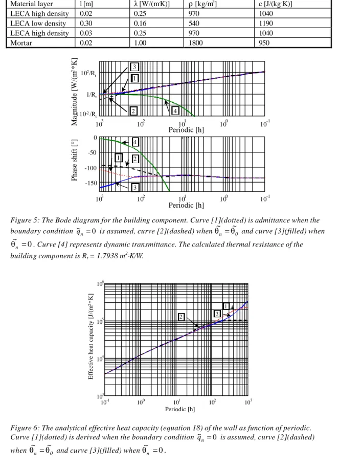
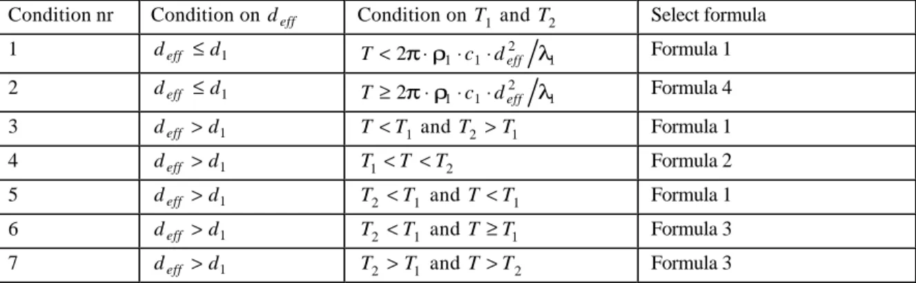
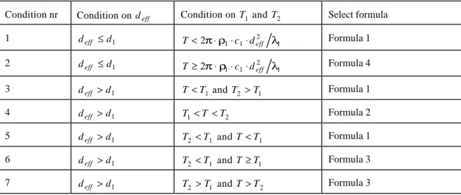
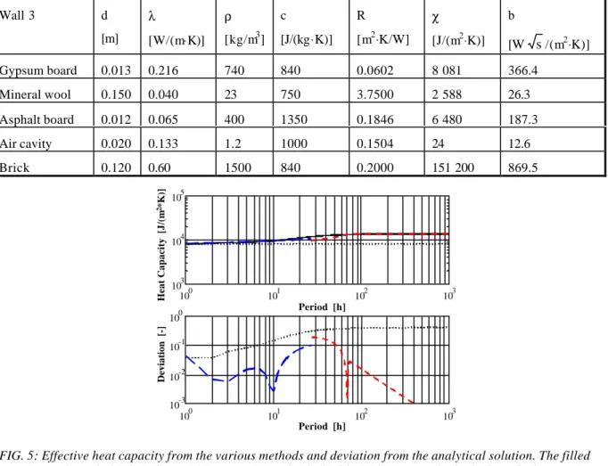
Results from one building component, the external wall facing North-Northeast, will be shown within this context. The wall is a massive type made of light expanded clay aggregates (LECA). Layer thickness and material properties are listed in table 3, and the thermal performance of the component is plotted in figure 5. The effective heat capacity was calculated for this component on basis of the surface heat capacity model, with results shown in figure 6.
Table 3: Layer thickness and material properties of a wall. The light expanded clay aggregate (LECA) material properties have been measured (SP 1996). The values of mortar are assumed.
Material layer l [m] λ [W/(m.K)] ρ [kg/m3] c [J/(kg.K)]
LECA high density 0.02 0.25 970 1040
LECA low density 0.30 0.16 540 1190
LECA high density 0.03 0.25 970 1040
Mortar 0.02 1.00 1800 950 10-1 100 101 102 103 10-2/R t 1/Rt 102/R t Magnitude [W/(m 2*K] Periodic [h] 10-1 100 101 102 103 -150 -100 -50 0 Phase shift [°] Periodic [h] 1 2 3 4 4 3 1 2
Figure 5: The Bode diagram for the building component. Curve [1](dotted) is admittance when the boundary condition ~qn =0 is assumed, curve [2](dashed) when θ~n =θ~0 and curve [3](filled) when
0 ~
= n
θ . Curve [4] represents dynamic transmittance. The calculated thermal resistance of the building component is Rt = 1.7938 m2⋅K/W. 10-1 100 101 102 103 103 104 105 106 Periodic [h]
Effective heat capacity [J/(m
2*K]
2
1 3
Figure 6: The analytical effective heat capacity (equation 18) of the wall as function of periodic. Curve [1](dotted) is derived when the boundary condition ~qn =0 is assumed, curve [2](dashed) when θ~n =θ~0 and curve [3](filled) when θ~n =0.
5.1.1 The measurement method
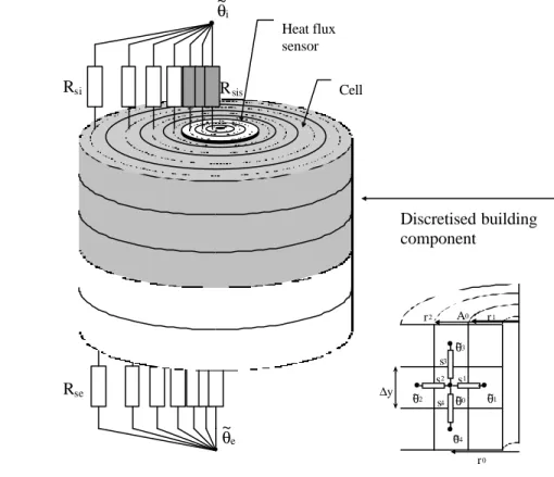
The measurements were made by means of the auxiliary wall method, commonly used to determine the thermal resistance of building components. In essence, a heat flux sensor is attached to a surface of the building component, usually on the internal surface. Next to this sensor, a thermocouple is placed on the internal and on the external surface. For measurement of the thermal resistance, data is collected during a number of weeks depending on the type of construction. Depending on how data is processed, the measurement time can be shortened by introducing statistical methods such as applied by
Anderlind (1996).
Within this project, the dynamic performance was to be monitored. The thermal excitation was primarily made with electrical radiators by means of a Pseudo Random Binary Sequence (PRBS), see for example (Jensen 1979). This pulse train of pre-determined zeros and ones contains a specific frequency spectrum, such that the frequencies in the internal environment are known.
The acquired data of a measurement series is transformed with Fast Fourier Transform (FFT) into the frequency domain, preceded by a calculation for determining the effective heat capacity for each frequency present in the PRBS. This measured result can then be compared to results obtained from analytical equations, provided that boundary conditions are the same in both cases.
5.1.2 The boundary conditions
Thus far in the theoretical calculations, the boundary conditions of the external surface have been assumed to be constant (θ~n =0 or q~n =0) or to have the same temperature oscillation as the internal surface (θ~n =θ~0). Now it may be expected that the measured temperature oscillation at the external surface does not fulfil these conditions. A calculation was made on the external wall (table 3) to study how the phase shift of θ~n θ~0 influenced the effective heat capacity. The magnitude of θ~n θ~0 was set to 1°C, while phase shift was varied in accordance to table 4. The influence was related to the effective heat capacity when the external surface temperature was assumed to be constant, such that
0 ~ 0 ~ ~ ~ = = − = n n 0 0 0 0 Y Y q θ θ θ δ (20)
From the results in figure 7, the conclusion is that phase shift in surface temperatures has a considerable influence on the effective heat capacity. An increase in amplitude of the external surface temperature oscillation will raise this effect, since the magnitude of the temperature ratio of this example is unity.
Table 4: Case number and boundary condition for calculation results shown in figure 7.
Case no. 1 2 3 4 5 6 7 8
0
n θ
10-1 100 101 102 103 -1 -0.8 -0.6 -0.4 -0.2 0 0.2 0.4 0.6 0.8 1 Period T [h] Relative influence of θ n / θ0 [-] ∼∼ 1 2 3 4 5 6 7 8
Figure 7: The relative influence δ (equation 20) of θn θ0
~ ~
on the effective heat capacity of the external wall as listed in table 3. Case number associated with each curve is defined in table 4. The amplitude of θ~n θ~0 is here assumed to be unity.
Within this experiment, it was wished to let temperatures and heat flows to be as ”natural” as possible. This means that the amplitude of the indoor temperature was not allowed to oscillate too much, as to measure the effective heat capacity in natural running conditions of a building, see for example the temperatures and heat flux measured at the surfaces of the external wall in figure 8. An amplification of the thermal loads in the internal environment may make thermal transmittance negligible.
500 1000 1500 2000 2500 3000 3500 4000 4500 5000 -5 0 5 10 Heat flux [W/m 2] 500 1000 1500 2000 2500 3000 3500 4000 4500 5000 -10 -5 0 5 10 Sample Temperatures [°C] 10-1 100 101 102 103 10-4 10-2 100 102 104 Magnitude Periodic [h] 1 2 3
Figure 8: To the left: Measured heat flux and temperatures at the wall surfaces (external dashed, internal filled). The mean value of each series has been subtracted. To the right: Power spectrum of heat flux [1], internal surface temperature [2] and external surface temperature [3].
5.1.3 Measured results in comparison with analytical results
A couple of results are shown here, but there are more in the paper 3. First, some notations will be defined. The effective heat capacities that are calculated from measured data are denoted by χ0* and
* B A χ as defined in equation 21. ω θ χ 0 0 0 q ~ ~ * =− ; ω θ θ θ χ 0 n 0 0 B A B q ~ ~ 1 ~ ~ * = − + ⋅ ; (21a)
The first measured effective heat capacity, χ0*, is the actual effective heat capacity of a building component in natural conditions, and is a direct application of the definition of admittance. The second type, χ*AB, has a compensation for dynamic transmittance as to make this measured entity directly comparable with the analytical entity χAB, which is calculated with the assumption that 0
~
= n
θ . The
analytical value, χ( )A 1− B, calculated with the assumption that θn θ0
~ ~
= is also shown in figures. The analytical heat capacities are defined as
ω χ B A B A = ; χ( ) ω B A B A 1 1 − = − (21b)
The deviations of measured values are related to the analytical value, such that
(
0 AB)
AB 0 χ χ χ δ = *− ; δAB =(
χAB−χAB)
χAB * (22)Figure 9 shows the measured and analytical effective heat capacities. The results are quite typical for other measurement locations: a noisy measured curve is situated somewhat lower than the theoretical curves. The data has in this case been sampled in a rectangular window.
10-1 100 101 102 103 103 104 105 106 Periodic T [h]
Effective heat capacity [J/(m
2*K)] 2 1 3 4 10-1 100 101 102 103 -1 -0.8 -0.6 -0.4 -0.2 0 0.2 0.4 0.6 0.8 1 Periodic T [h] Deviation [-] 1 2
Figure 9: Results from the external wall based on data sampled from a rectangular window. To the left: Measured effective heat capacities χ0* [1] and χ*AB [2] (equation 21a), analytical effective
heat capacities χAB [3] and χ( )A 1− B [4](equation 21b). To the right: Deviation between
experimental and theoretical values, δ [1] and 0 δAB[2] (equation 22).
On sampling the data in a Hanning window (Ramirez 1985), the measured results change form since the Hanning window has the effect of ”smoothing” frequency data.
The curves of figure 10 are actually quite representative for results obtained for other components and measurement points. At high frequencies, it is typical for the deviation curves to be situated in the regions of -40%. As period increases, deviation steadily approaches zero at the periodicity of around 10 to 20 hours. For longer periods, the measurement values oscillate with large magnitudes in an irregular fashion around the zero deviation line.
10-1 100 101 102 103 103 104 105 106 Periodic T [h]
Effective heat capacity [J/(m
2*K)] 2 1 3 4 10-1 100 101 102 103 -1 -0.8 -0.6 -0.4 -0.2 0 0.2 0.4 0.6 0.8 1 Periodic T [h] Deviation [-] 1 2
Figure 10: Results from the external wall based on data sampled from the Hanning window. To the left: Measured effective heat capacities χ0* [1] and χ*AB [2](equation 21a) and analytical effective
heat capacities χAB [3] and χ( )A 1− B [4] (equation 21b). To the right: Deviation between
experimental and theoretical values, δ [1] and 0 δAB[2] (equation 22).
5.1.4 Reasons for deviation in analytical and experimental results
These deviations can be explained. The systematic deviations at higher frequencies (below some 10 hour periodic) are mainly due to the heat flux sensor. Two finite difference programs calculating in the frequency domain were produced, using the calculation procedure as proposed by Andersson and Jóhannesson (1983). The first program models a homogeneous round slab placed on the surface of a cylindrical building component section. Calculations were performed as to determine how the circular sensor distorts heat flux at the wall surface. The second finite difference program, with Cartesian co-ordinates, models the central sensitive parts of a heat flux sensor composed of half-plated wound wire thermopiles. The temperature difference across the sensor is measured at the junction of the plated and non-plated part of the wire. Calibration is made at stead-state, and the heat flow through the sensor is directly proportional to the temperature difference. However, under the influence of dynamic processes, heat waves will be transmitted faster through the wire than through the plastic filling. The measured temperature difference will not conform to the heat flow through the sensor.
Some of the results from simulations are plotted in figure 11. The deviation is defined on basis of the “measured” heat flux in relation to the heat flux at an undisturbed section of the wall, such that
wall wall measured q q q ~ ~ ~ − = ε (23)
Note that the design of the heat flux sensors that were used were not know; the results of figure 11 are based on a hypothetical design with exception to material properties, wire diameter and sensor thickness. However, the results indicate that the magnitude of effective heat capacity deviations in the previous section are of the order that may be expected for a heat flux sensor in dynamic conditions. Therefore, it is the influence of the measurement organ itself, the thermopile, that leads to the systematic deviations below frequencies corresponding to the 10 to 20 h periodic. Also note that other sources of inaccuracies, such as calibration inaccuracies (±5%), are not taken into consideration.
-0.2 10-1 100 101 102 103 -0.4 -0.35 -0.3 -0.25 -0.15 -0.1 -0.05 0 Deviation ε [-] Period T [h]
Figure 11: The two curves displays simulated deviation ε (equation 23) between "measured” heat flux and heat flux at an undisturbed wall surface. The curve with triangles displays results from a circular homogeneous slab composed of polyurethane, which is a common sensor filling material. The curve with rings shows results from a simulated central section of a heat flux sensor that contains constantan wire (the thermopile). Thus, the thermopile itself stands for a substantial part of deviations.
The discrepancies at wave lengths larger than some 10 hours can be motivated by what is happening at the external surface. The phase shift in temperature oscillations (or thermal transmittance) has an impact on the effective heat capacity. However, this is not the whole truth, because a better agreement would be expected between compensated measured values and analytical values, as evaluated by δAB. The reason is the handling of measured data with FFT.
FFT assumes a periodicity in the sampled window: this window repeats itself in time. This means that the value at the start of the series should be the same as the last value of the series. For this to be possible, all frequencies within the window have to be integer multiples of the fundamental periodic, which is the length of the window. This is difficult to achieve in field measurements. If one or several frequency components are not integer multiples of the fundamental frequency, the use of FFT will lead to leakage (Ramirez 1985). Leakage occurs in the power spectrum, where the energy of one frequency component leaks to neighbouring frequencies. A problem is that the frequencies in the internal environment (the frequencies of the PRBS), which are used within the calculations, are not identical to frequencies present in the external environment. The energy of the frequencies present in the external environment will be distributed (leak) among the frequencies used in the calculations. In turn, the leakage at lower frequencies of the external environment may give rise to erroneous dynamic transmittance.
5.2 The approximate method
A new approximate method has been developed to determine the effective heat capacity of a multilayer building component, with definition based on the surface heat capacity model. In this method, only real numbers are used within the calculations, and these are founded on the thermal properties and
thickness of the material layers. The new method gives more accurate results over a wider range of frequencies than the approximate methods of normative Annex A of prEN ISO 13786 (1998). A drawback is that the new method requires more work to produce the results than that of prEN ISO 13786. On the other hand, experience indicates that the inaccuracy seldom is larger than some 15 % and commonly less than 10 %. The approximate methods of prEN ISO 13786 give values that can have larger discrepancies than 50%, which makes any calculations with this method less worthwhile. Calculations with the new method require calculators, spreadsheet programs or mathematical programs that do not handle complex numbers.
The method is stated here, but the reader is advised to view Paper 2 for examples on application.
The new approximate method
The method consists of 5 calculation steps in junction with three tables. The first table lists the nomenclature of symbols used in the calculation procedure.
TAB. 1: Nomenclature and definitions.
Symbol Unit Comments
j Index Layer number. 1 is the internal surface material, n the external surface material. j
d m Thickness of material layer j.
j
λ W/(m⋅K) Thermal conductivity of material layer j.
j
ρ kg/m3 Density of material layer j.
j
c J/(kg⋅K) Specific heat capacity of material layer j.
j
R m2⋅K/W Thermal resistance of material layer j, Rj =dj λj j
χ J/(m2⋅K) Heat capacity of material layer j, χj =dj⋅ρj⋅cj j
b W⋅ s/( m2⋅
K) Thermal effusivity of material layer j, bj = λj⋅ρj⋅cj
1. Acquire material data (λ ,j ρ and j c ) and geometry (j d ) of each material. Calculate j R , j χ andj j
b for each layer j. Choose the time period T for which the areic heat capacity is to be calculated. The angular frequency ω (s-1) is given by
T π
ω 2= (24)
2. Determine the maximum areic heat capacity χ for the considered surface according toc0
0 , 2 1 1 1 1 1 = + ⋅ = + = + + =
∑
∑
n n j n j k k j j t c0 R R R R χ χ ;∑
= = n j j t R R 1 (25)3. Calculate the effective thickness deff by means of χ . The number of layers x at the inner sidec0 of the adiabatic plane is established.
∑
= ⋅ ⋅ = x j j j j c0 c d 1 ρχ such that eff
x j j d d =
∑
=1 (26)The thickness of layer x can be adjusted to the length
∑
− = − 1 1 x j j eff d d .4. Calculate time period values T and 1 T (2 T is omitted for slabs) according to2
1 1 1=2π⋅R ⋅χ T and
(
)
(
)
2 2 1 2 2 1 1 2 1 2 2 1 2 2 2 1 4 − + + − + ⋅ = χ χ χ χ χ χ χ π b T (27)Selection of formula for χ is based on fulfilment of criteria for the size of c deff , T and 1 T in2 TAB. 2.