FInancial development and economic growth: cross-country comparisons.

(1)

Financial development and economic

growth: cross-country comparisons.

Paper within MASTER THESIS IN ECONOMICS Author: KRASULINA NATALIA

Tutor: AGOSTINO MANDUCHI

(2)

ABSRACT

This study attempts to investigate the relationship between financial development and eco-nomic growth and also the empirical analysis examines Granger causality of this relationship. Time series models are applied for six countries with emerging markets and different types of financial system (Saudi Arabia, Kuwait, Tunisia, Morocco, Israel and Egypt). For the pair-wise combinations of financial development indicators and economic growth which do not have cointegrating relationships, Granger causality is applied within the vector autoregressive (VAR) model. When the variables have cointegrating relationship, Granger causality test is applied using the vector error correction model (VECM). The empirical results in the study case suggest that financial structure in some degree can explain economic growth indicator. Moreover the test results show weak dependence between financial development and econom-ic growth. The Granger causality test indeconom-icates unidirectional Granger causality running from financial development and economic growth, reverse relationship and bidirectional Granger causality.

(3)

1 INTRODUCTION ... 1

2 BACKGROUND ... 3

2.1 Theoretical framework ... 3

2.2 Empirical evidence ... 4

2.2.1 The role of financial structure ... 4

2.2.2 Financial development and economic growth ... 5

3 DATA SPECIFICATION AND METHODOLOGICAL ISSUES ... 7

3.1 Country Selection ... 7

3.2 Indicators of financial development and economic growth ... 8

3.3 Methodology ... 11

4 EMPIRICAL RESULTS ... 14

4.1 The results of the preliminary steps ... 14

4.2 Granger causality test for non-cointegrated variables ... 15

4.3 Granger causality test for cointegrated variables ... 18

5 CONCLUDING REMARKS ... 21

REFERENCES ... 23

(4)

1 INTRODUCTION

Economic growth is a positive change in the level of production of goods and services of a country over a certain time period. Generally accepted economics suggest that growth in the quantities available of factors of production such as labor, capital and land are the main de-terminants of growth. In the course of time some economists include also the financial devel-opment as a factor of economic growth.

The relationship between financial development and economic growth has been the subject of increasing attention over the 20th century. There are still old disputes concerning the direction of causality between financial development and economic growth, the power of influence and the way of financial factors’ impact.

Another issue of this topic is: does the type of financial system matter for economic growth? In the economic literature there is no single answer to the question of what is better for eco-nomic growth: the banks, the stock market or neither. As it is well known, all the financial systems of all countries depend on the predominant mechanism of mobilizing resources for investment. Due to this the financial system can be divided into two main categories: 1) the bank-based financial system and 2) the market-based financial system.

In the bank-based financial system banks play a significant role in firms’ financing, allocating resources, mobilizing savings. The process of investment and allocation of resources occurs through the bank loans, which are a major share of external financing of firms. According to the market-based financial system, financial markets such as securities market, stock market and etc., play an important role in providing financial services. In this case firms rely primari-ly on the stock markets by issuing shares and bonds in free circulation.

Recently the study of the financial development as an engine of economic growth and investi-gation of importance of financial systems has been considered by a number of articles. Even though there are not plenty of studies that examine the financial structure by using time series technique. Moreover, countries that are considered in this work have not been tested from this point of view.

The countries I choose are Saudi Arabia, Kuwait, Tunisia, Morocco, Israel and Egypt. The se-lection of these countries was based on an analysis that has been made concerning two indi-ces. Furthermore, in this study case Saudi Arabia and Kuwait are taken as countries with a market-based financial system, Tunisia and Morocco – a bank-based financial system, Israel and Egypt – a diversified financial system.

The purpose of this work is to investigate the relationship between economic growth and fi-nancial development and if there is any relationship, it is relevant to check for the existence of Granger causality.

So the problems that will be examined are the following:

 Is there any existent relationship between financial development and economic growth in the chosen countries?

(5)

 Is there any Granger causal relationship between indicators of financial devel-opment and economic growth?

 Do different financial systems have a different impact on economic growth? The rest of the work is organized as follows. The background of the topic is presented in sec-tion 2, both theoretical and empirical evidences. Section 3 defines the proxies of financial de-velopment and economic growth, discusses the econometric specification and indicates the country selection for the time series analysis. The main empirical results of the research are presented in section 4. Finally, section 5 describes the conclusion that can be drawn.

(6)

2 BACKGROUND

This section provides some literature reviews of two main issues: 1) analysing different forms of financial systems; 2) investigations concerning the relationship between financial devel-opment and economic growth. There is a set of theoretical and empirical study cases of the relative merits of market-based and bank-based financial systems. Allen and Gale (2000) pro-vide a broad spectrum of literature review pertinent to this topic. In regard to relationship be-tween financial development and economic growth plenty of studies both theoretical and em-pirical have been done starting by Schumpeter (1911), Gurley and Shaw (1955, 1960).

2.1 Theoretical framework

Some economists argue that the banking system finances industrial development more effectively than market system (Gerschenkron (1962), Rajan and Zingales (1998), Stulz (2000)). On the contrary, Levine and Zervos (1998) argue that stock markets have a positive role in allocating resources, corporate governance, strengthening risk management and etc. They assumed that more market-based financial system provides basic financial services that stimulate long-run economic growth.

Another conventional and basic issue of this topic is the causal relationship between financial development and economic growth. Earlier study by Bagehot (1873) argues the financial system played an important role in the conception of industrialization in England by promoting capital formation for the “immense work”. Many others studies indicate that financial development is correlated with current and future economic growth, physical capital accumulation and economic efficiency. In this case the financial development may cause economic growth.

On the contrary, authors such as Robinson (1952) and Kuznets (1955) argue that economic growth causes financial development and financial development simply follows economic growth.

Patrick (1966) introduced the idea of the bi-directional relationship between financial development and economic growth, suggested “supply-leading” and “demand-following” patterns. In the “supply-leading” role, the financial development causes economic growth. Patrick describes the functions of this phenomenon as follows: “to transfer resources from traditional (non-growth) sector to modern sectors, and to promote and stimulate an entrepreneurial response in these modern sectors”. In other words, financial intermediation allocates resources to more productive sectors.

In the “demand following” role economic growth causes financial development. According to Patrick, “the creation of modern financial institutions, their financial assets and liabilities, and related financial services is in response to the demand for these services by investors and savers in the real economy”. The increasing demand for financial services might lead to the expansion of the financial system as the real sector of the economy.

(7)

2.2 Empirical evidence

The main approaches to testing the correlation between financial development and economic growth are:

1) cross-section or panel data techniques for testing the group of countries; 2) industry-level or firm-level evidence;

3) time series techniques for testing the hypothesis for a particular country. We will highlight just more relevant studies according to stated questions

2.2.1 The role of financial structure

In this subsection the studies which investigate the relationship between different financial structures and economic growth are described. Some works conclude that there is no connec-tion between the bank-based or market-based financial systems with economic growth. For example, Levine (2002) examines which financial systems are better in supporting eco-nomic growth by using cross-country technique. The empirical findings present that “although overall financial development is robustly linked with economic growth, there is no support for either the bank-based or market-based view”.

The work by Beck and Levine (2002) can be presented as another example. They analyze whether market-based or bank-based financial systems have impact on improving the effi-ciency of capital allocation across industries and influence industries’ expansion. As opposed to the previous study the industry level analysis is applied for 42 countries and 36 industries. The empirical results show that neither the market-based nor the bank-based financial system can explain industrial growth or the efficiency of capital allocation.

On the contrary, the studies based on the time series technique indicate that different types of financial structure promote economic growth. Arestis, Luintel D., and Luintel B. (2005) ana-lyze whether financial structure influences economic growth. In the work three views of fi-nancial system is highlighted: the bank-based, the market-based and the fifi-nancial services view. The empirical issue is tested by time series data and Dynamic Heterogeneous Panel ap-proach on developing countries. The results indicate “significant cross-country heterogeneity in the dynamics of financial structure and economic growth”. The time series results present that financial structure significantly explains economic growth.

Lee (2012) reexamines the relationship between financial structure and economic growth. By testing the different countries that were not tested in previous analyzed work he found that different financial systems promote long run economic growth. Except of one country, all others show that the financial development Granger causes economic growth.

The preliminary study about different types of financial systems can help with understanding this issue, the work by Demitguc-Kunt and Levine (1999) can be highlighted. They analyze advantages and disadvantages of bank-based and market-based financial systems. They com-pare German and Japan as bank-based countries and England and the United States as market-based financial systems. They found that “bank, nonbanks, and stock markets are larger, more

(8)

active, and more efficient in richer countries. In higher income countries, stock markets be-come more active and efficient relative to banks”.

2.2.2 Financial development and economic growth

Most studies conclude that there is a positive relationship between financial development in-dicators and economic growth. For example, Goldsmith (1969) and King and Levine (1993) empirically examine the relationship between financial development and economic growth for a set of countries. The difference between these two works is that different proxies of finan-cial development and different sets of countries are used. Nevertheless their empirical results indicate a strong positive relationship between financial development indicators and economic growth indicators.

Levine and Zervos (1998) examine whether stock market and banking development correlated with current and future rates of economic growth. The empirical findings suggest that the lev-el of stock market liquidity and banking devlev-elopment are positivlev-ely and significantly corrlev-elat- correlat-ed with rates of economic growth, capital accumulation, and productivity growth. Lately Lev-ine, Loyaza and Beck (2000) investigate whether the exogenous component of financial in-termediary development influences economic growth.

At the industry and firm levels studies investigate the performance of financial sector and in-dustrial or firm growth. The positive unidirectional causality running from financial develop-ment to industrial growth has been found. For example, Rajan and Zingales (1998) examines whether financial-sector development has an influence on industrial growth. Demirguc-Kunt and Maksimovic (1998) examine whether the financial development influences firms’ deci-sion of investing in potentially profitable growth opportunities. In this study they also “focus on the use of long-term debt or external equity to fund growth”.

Within time series technique, Acaravci at al (2007) test the causal relationship between two proxies of financial development and economic growth. The empirical findings indicate that there is no long-run relationship between financial indicators and economic growth. Moreo-ver, it should be indicated that the results show a one-way causal relationship from the finan-cial development to economic growth. The same methodology will be used in this paper. On the contrary, some studies indicate not only causality running from financial development to economic growth, but also the reverse and bidirectional causality. The main prove of this fact is the work by Demetriades and Hussein (1996). They examine 16 countries by using time series technique.

Abu-Bader and Abu-Qarn (2008) investigate the causal relationship between financial devel-opment and economic growth for six Middle Eastern and North African countries (Algeria, Egypt, Morocco, Israel, Tunisia and Syria). They applied quadvariate vector autoregressive framework and Granger causality test. The empirical findings show strong causal relationship from financial development and economic growth. But in case of Israel the results imply “weak support for causality running from economic growth to financial development but no causality in the other direction”.

(9)

Within the time series technique some studies show only Granger causality running from eco-nomic growth to the development of financial intermediaries. For example Guryay, Safakli and Tuzel (2007) in their work made the same conclusion by examining this relationship in Northern Cyprus.

(10)

3 DATA SPECIFICATION AND METHODOLOGICAL

ISSUES

3.1 Country Selection

Financial systems vary across different countries. Most countries have banking system and fi-nancial markets, but in different countries these fifi-nancial institutions play different roles. Some countries have the market based financial system; others have the financial system that is oriented to the banking institutions. The country selection in this research will be based on different forms of financial system.

There are no generally adopted rules for defining the bank based and the market based finan-cial system. In this case it is necessary to provide measures, which can partly show the form of the financial system. Based on Levine (2002) we can compute new rankings by providing “structure-activity” and “structure-size” indices for 50 countries over the 1995-2009 period (15 years changes). The country choice is based on data availability.

“Structure-activity” shows “the activity of stock markets relative to that of banks”. For meas-uring the activity of stock markets the ratio of total value stock traded are used which equals the total value of shares traded during the period divided by GDP. This ratio indicates market liquidity by the reason of measuring trading in the market relative to economic activity. As indicator of banks activity, the bank credit ratio can be used. This measure equals the value of domestic credit provided by banking sector as a share of GDP. To calculate “structure-activity” index it is necessary to take the natural logarithm of the total value stocks traded to GDP divided by domestic credit provided by banking sector to GDP.

“Structure-activity” index = ln ( 𝑠𝑡𝑜𝑐𝑘 𝑡𝑟𝑎𝑑𝑒𝑑 ,𝑡𝑜𝑡𝑎𝑙 𝑣𝑎𝑙𝑢𝑒 (𝑎𝑠 𝑠𝑕𝑎𝑟𝑒 𝑜𝑓 𝐺𝐷𝑃)_{𝐵𝑎𝑛𝑘 𝑐𝑟𝑒𝑑𝑖𝑡 (𝑎𝑠 𝑠𝑕𝑎𝑟𝑒 𝑜𝑓 𝐺𝐷𝑃)} )

Higher values of this index imply a more market based financial system. The values are ranked and presented in table 1 (see Appendix).

“Structure-size” index indicates the size of performance of stock markets relative to that of banks. The market capitalization ratio indicates the size of domestic stock market. As in the previous case to measure the size of banking system the bank credit ratio is used. “Structure-size” index equals the natural logarithm of the market capitalization to GDP divided by do-mestic credit provided by banking sector to GDP.

“Strucure-size” index = ln( 𝑀𝑎𝑟𝑘𝑒𝑡 𝑐𝑎𝑝𝑖𝑡𝑎𝑙𝑖𝑧𝑎𝑡𝑖𝑜𝑛 (𝑎𝑠 % 𝑜𝑓 𝐺𝐷𝑃)

𝐵𝑎𝑛𝑘 𝑐𝑟𝑒𝑑𝑖𝑡 ( 𝑎𝑠 𝑠𝑕𝑎𝑟𝑒 𝑜𝑓 𝐺𝐷𝑃) )

The same logic can be applied for this index, the greater value the more market based system. These indices should be very carefully interpreted by the reason of some abnormal results. The values are ranked and presented in table 1 (see Appendix).

According to calculated rankings, it can be assumed that Saudi Arabia, Singapore, Finland, Switzerland, Kuwait have more market based financial system. These countries are on top of both rankings. On the contrary, Tunisia, Cyprus, Sri Lanka, Slovenia and Morocco are situat-ed below the mean of rankings. By this reason, we can argue that these countries have more

(11)

bank-based financial systems. Moreover, countries as Israel, Egypt, Indonesia, and Poland in the ranking are close to the mean, so these countries have more diversified financial systems. Based on conclusions above we can choose countries according to the different financial sys-tems and data availability. The six countries with emerging markets are applied in current analysis: 1) market-oriented financial system (Saudi Arabia, Kuwait); 2) bank-based financial system (Tunisia, Morocco); 3) diversified financial system (Israel, Egypt). To sum up, the Table 2 below observes the list of chosen countries with corresponding time period and num-ber of observations.

According chosen countries we can observe some similarities and differencies. It should be mentioned that all countries except Israel have Islamic Banking system. This type of banking is based on Islamic Law (Sharia ) that prohibits a set of banking operation such as: the fixed of floating payment, acceptance of interest of futures and forwards contracts. Another princi-ple of following Islamic Banking is that it is not allowed to invest in businesses that are di-verged according Islamic law. Such areas can be alcohol or drug production and etc. 1

Table 2 The list of countries

Country

Period

This ratio reflects the financial resources provided to private sector such as loans, trade credits and etc. It is assumed that this ratio generates increases in investment to much larger extent than credits to public sector. Also I can conclude that loans to the private sector are improving the quality of investment as soon as financial intermediaries’ more stringently evaluation of project viability.

Another proxy of financial development that can be used is the ratio of private sector credit to domestic credit. The formula of this indicator is the following:

Proxy 4 =

𝐷𝑜𝑚𝑒𝑠𝑡𝑖𝑐 𝑐𝑟𝑒𝑑𝑖𝑡 𝑡𝑜 𝑝𝑟𝑖𝑣𝑎𝑡𝑒 𝑠𝑒𝑐𝑡𝑜𝑟

𝐷𝑜𝑚𝑒𝑠𝑡𝑖𝑐 𝑐𝑟𝑒𝑑𝑖𝑡 𝑝𝑟𝑜𝑣𝑖𝑑𝑒𝑑 𝑏𝑦 𝑏𝑎𝑛𝑘𝑖𝑛𝑔 𝑠𝑒𝑐𝑡𝑜𝑟

∗ 100

This indicator reflects the domestic assets distribution of an economy and also it computes the proportion of credit allocated to private enterprises by the financial system. By using this ratio it can be concluded if the financial intermediations can satisfied the private sector’s claims or not.

The ratio of private sector credit to domestic credit and the private sector credit ratio still have some problems. Both indicators do not indicate the degree of public sector borrowing; they just reflect the private sector’s demand. In spite of the criticism we can assume that this num-ber of financial indicators can be used to maximize the information of financial development. In the case of the indicator for economic growth, there are some common proxies that have been used, For example, King and Levine (1993) apply four indicators for economic growth: “real per capita GDP, the rate of physical capital accumulation, the ratio of domestic invest-ment to GDP, a residual measure of improveinvest-ments in the efficiency of physical capital alloca-tion”. Demetriades and Hussein (1996) use real GDP per capita as an indicator of economic development, but they measure this variable in domestic currency. The analyses of Kar and Pentecost (2000) and Unalmis (2002) were based on Gross National Product (GNP) at current prices as proxy for economic growth.

In our study I will use real GDP per capita on U.S. dollars. The definition of The World Data is: “GDP is the sum of gross value added by all resident producers in the economy plus any product taxes and minus any subsidies not included in the value of the products divided by midyear population”. This measure evaluates the activity of an economy, and by using this indicator for all the chosen countries on the same currency (U.S. dollars) we can properly compare the results. Another advantage of this proxy is that the population differences are al-so included in this indicator, al-so the correct estimations can be computed. But GDP per capita does not reflect the distribution of the resources of the economy.

All the data is taken from the World DataBank, World Development Indicators & Global De-velopment Finance. Table 3 indicates the summarizing information about the data and also provides the notation for the present analysis.

(14)

Table 3 Variables’ notations.

Indicator

Notation

GDP per capita Y

Broad money supply ratio M2

Banking credit ratio BC

Private credit ratio PC

Private credit to banking credit ratio PC/BC

3.3 Methodology

In order to empirically test the causal relationship between financial development and eco-nomic growth it is common to apply Granger causality test (Granger (1969), Sims (1972)). This test provides a “useful way of describing the relationship between two (or more) varia-bles when one is causing the other(s)”3

. Moreover, the cointegration technique (Engle and Granger (1987)) provides us with more informative results about the causal relations. Accord-ing to this technique, Engle and Granger (1987) argue that if two (or more) variables are found to be cointegrated, there is a corresponding error-correction representation.

The basic concept of the empirical investigation is to estimate a simple bivariate model (pair-wise combination between economic growth (Y) and the four proxies of financial develop-ment (FD)). The first step in this study is to test the variables for unit root. For this purpose the Augmented Dickey Fuller test will be used.

The testing procedure for this test is applied to the following regression:

ΔY

t

= β

1

+β

2

t+δY

t-1

+α

1

ΔY

t-1

+…+ α

p-1

ΔY

t-p+1

+ε

t

where β1 is a constant, β2 the coefficient on a time trend, p the lag of order of the autoregres-sive process, εt – is a pure white noise error term.

The Augmented Dickey Fuller is estimated in three different forms:

1) β1 and β2 equal 0 corresponds to modeling a random walk (ΔYt

= δY

t-1

+ε

t

)

2) β2=0 corresponds to modeling a random walk with a drift (ΔYt

= β

1

+δY

t-1

+ε

t

trend.

3

Granger, C.W.J. (1969). "Investigating Causal Relations by Econometric Models and Cross- Spectral Methods,'

(15)

The null hypothesis is that δ=0, so there is a unit root and the time series is non stationary. The alternative hypothesis is that δ less than zero, so the time series dataset is stationary. If the test statistic is less that the critical value, then the null hypothesis can be rejected. It means that there is no unit root and the time series is stationary.

If all the variables turn out to be integrated of the same order, it is necessary to check for cointegrating relationship between these variables. For this purpose we will apply Johansen cointegration test.

If two time-series are non stationary, but their linear combination is stationary, it is called as the cointegrating equation and can be interpreted as a long run equilibrium relationship among two chosen time series. The purpose of Johansen cointegration test is to determine whether a group of non-stationary series is cointegrated or not. This methodology is based on the VAR model of order p:

y

t

= A

1

y

t-1

+…+ A

p

Y

t-p

+ Bx

t

+ ε

t

12.2

Y

t-2

t-2

+…

+ β

2p.2

Y

t-p

+e

t2

+µ

21.2

ΔY

t-1

+

+ µ

22.2

ΔY

t-2

+…+ µ

2p-1.2

ΔY

t-(p-1)

+ δ

2

EC

t-1

+ γ

t2

where EC is the error correction term, p is the order of the VAR, π is the constant term, γ is an error term, FD denotes proxy of financial development and Y denotes economic growth. As a final step, the models will be tested for non-causality. First, we test for the non-causality between the non-stationary and non-cointegrated variables. By working with the first differ-ence we test for the joint significance of the coefficients of the lagged variables using a Like-lihood Ratio test.

Next we will test for the non-causality between non-stationary and cointegrated variables. Firstly t-test will be used for determining the significance of the error correction term, second-ly, we test for joint significance of the lagged variables and finally joint significance of the lagged variables and the error correction term is examined.

In this study unidirectional Granger causality suggests that financial development Granger causes economic growth. On the contrary, reverse Granger causality means that indicator of economic growth influences financial development. And finally, when financial development and economic growth cause each other we can assume that there is bidirectional Granger cau-sality.

(17)

4 EMPIRICAL RESULTS

4.1 The results of the preliminary steps

The empirical results of Augmented Dickey Fuller test indicate that for Saudi Arabia and Egypt the cointegration test will not be applied because the variables are not integrated of the same order. The pairwise combinations of financial development and economic growth indi-cators of the four other countries (Kuwait, Tunisia, Morocco and Israel) can be tested for ex-istence of cointegrating relationship.

Johansen cointegration test indicates overall four cointegrating relationship over four coun-tries. In case of Tunisia none of this relationship is observed after applying Johansen cointegration test. For Kuwait and Israel only one cointegration relation is indicated. And fi-nally in case of Morocco two long-run pairwise relationships can be presented. For the de-scribed above cointegrating variables VECM will be applied. On the contrary, for the rest of pairwise combinations VAR model will be used. The empirical outputs of Augmented Dickey Fuller and Johansen cointegration tests will be considered below in more details.

Table 4 observes the result of Augmented Dickey Fuller test for Saudi Arabia. All the varia-bles except of GDP per capita do not fluctuate over the time. In this case we applied third form of the test, where there is a random walk with drift around stochastic trend. GDP per capita indicates the stable growth over time, thereby the second form was applied. The empir-ical findings show that all the variables except of Y integrated of order 0. To sum up, it can be conclude that in case of Saudi Arabia we will work with VAR model, preliminarily taking the first difference of Y (DY).

Table 5 indicates the empirical results of the unit root test for Kuwait. All the variables except of PC/BC show the growth over the given period. In the case of Y, we can observe more sig-nificant increase. Moreover, all the variables are integrated of order 1, so Johansen cointegration test can be applied in this case. According all above, in case of Kuwait (Table 10) we can conclude that only broad money supply ratio (M2) and Y have long-run relation-ship. For other pairwise combination of financial proxies and economic growth indicators the cointegration test does not indicate any cointegrating vectors. In latter case VAR model will be implied.

The next analyzed countries are Tunisia and Morocco (Table 6 and Table 7). All the variables for each country show the stable growth over the time. Moreover, all the variables integrated of the same order, so as in the previous case the cointegration test can be computed in these cases. Although we can observe different results of Johansen cointegration test.

For Tunisia (Table 11) Johansen cointegration test does not indicate any long run relationship between financial development measures and economic growth indicator. As in the previous situation VAR model will be used for determining whether there is any Granger causal rela-tionship or not.

In case of Morocco (Table12) this test concludes that there are two combinations of Y and proxies of financial development that indicate cointegrating relationship: 1) Y and banking credit ratio (BC); 2) Y and broad money supply ratio (M2). For these pairwise combinations

(18)

VECM will be implied. For others variables bivariate VAR model will estimated for deter-mining Granger causal relationships.

In case of Israel ( Table 8) it can be observed that all the t-statistic value of the first difference are significant at 5 % level, all the variables are integrated of order 1. Johansen cointegration test for Israel (Table 13) indicates only one cointegrating relationship between PC/BC and Y. So, for this set of variables VECM will be applied.

And finally in case of Egypt (Table 9) only one variable is integrated of order 1, others are in-tegrated of order two. By the reason that Y is inin-tegrated of different order from other variables we cannot apply Johansen cointegration test.

4.2 Granger causality test for non-cointegrated variables

If the combination of non-stationary variables has no cointegrating relationship or if depend-ent variable and independdepend-ent variables are integrated of differdepend-ent order, VAR model should be applied. Before estimating this model two preliminary steps should be taken:

1) make the variables stationary by taking first or second difference, depending on the result of unit root test;

2) determine an optimal lag length by using information criterion like Akaike information cri-terion.

The estimation of bivariate VAR models is not relevant in this study, but we are interested in the direction of causality. After determining the order of VAR model, we can proceed to the Granger causality test. According to Augmented Dickey Fuller and Johansen cointegration tests, which are discussed above, we can conclude that for all pairwise combination of the var-iables of Saudi Arabia and Egypt, Granger causality test can be applied. For other countries this test will not be used for all combinations of variables. More details will be provided fur-ther.

Granger causality test is applied for the following directions:

 Direction 1 - from financial development to economic growth;

 Direction 2 – from economic growth to financial development.

The null hypothesis for both directions is: Ho – the first variable does not Granger cause an-other variable. On the contrary, the alternative hypothesis means, that the first variable do Granger cause other variable.

After applying Granger Causality test, I can assume that there is a weak pattern between fi-nancial structure and economic growth. It can be observed that in two cases economic growth variable has impact on Private credit ratio (PC). In the three cases out of six, broad money supply (M2) Granger causes economic growth. Banking credit ratio (BC) has causal relation-ship with economic growth in two countries (Tunisia and Israel). This result can be expected by the reason that Tunisia has more bank based financial system, so the banking sector has an

(19)

impact of economic development in country, and in case of Israel, I can argue that the bank-ing system is quite developed, so it can influence economic performance. More detailed anal-ysis is presented below.

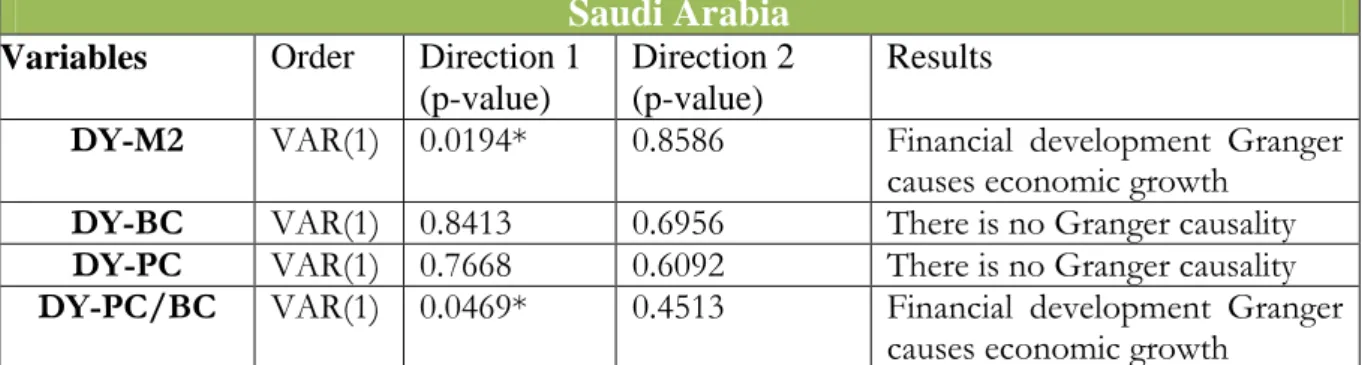
Table 14 below presents the empirical results of Granger causality test for Saudi Arabia. As you can observe, this test indicates only two Granger causal relationships from financial de-velopment variables to economic growth: Broad money supply ratio (M2) and Private credit to Banking credit ratio (PC/BC) Granger cause GDP per capita (Y). The others combinations of variables do not show any Granger causality.

Table 14 Granger causality results for Saudi Arabia

Saudi Arabia

Variables Order Direction 1

(p-value)

Direction 2 (p-value)

Results

DY-M2 VAR(1) 0.0194* 0.8586 Financial development Granger

causes economic growth

DY-BC VAR(1) 0.8413 0.6956 There is no Granger causality

DY-PC VAR(1) 0.7668 0.6092 There is no Granger causality

DY-PC/BC VAR(1) 0.0469* 0.4513 Financial development Granger

causes economic growth Notes: * - significance level of 5%

D indicates first difference of the variable Source: Author’s calculations

The next analyzed country is Kuwait (Table 15). Granger causality test represents different results from the findings for Saudi Arabia. As you can see, in this case the indicator of eco-nomic growth Granger causes Private Credit ratio (PC). The correlation between these two variables is equals 0.50, so we can admit that there is a positive correlation. Moreover we can conclude that if GDP per capita is increasing, private credit ratio (PC) will also grow.

Table 15 Granger causality results for Kuwait

Kuwait

(p-value)

Results

DY-DBC VAR(2) 0.8218 0.2152 There is no Granger causality

DY-DPC VAR(1) 0.3805 0.0443* Economic growth Granger

causes financial development

DY-D(PC/BC) VAR(2) 0.7066 0.8635 There is no Granger causality

Notes: * - significance level of 5% D indicates first difference of the variable Source: Author’s calculations

(20)

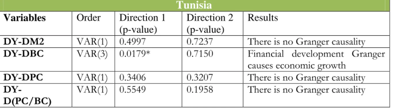
In case of Tunisia (Table 16) we can observe the only Granger causality between Banking Credit ratio (BC) and economic growth indicator. If financial development indicator changes over the time, GDP per capita will also change. The correlation indicates positive relationship (0. 65) between these variables.

Table 16 Granger causality results for Tunisia

Tunisia

(p-value)

Results

DY-DM2 VAR(1) 0.4997 0.7237 There is no Granger causality

DY-DBC VAR(3) 0.0179* 0.7150 Financial development Granger

DY-DPC VAR(1) 0.3406 0.3207 There is no Granger causality

Table 17 below shows the result of Granger causality test for Morocco. In this case we can observe interesting result – there is bidirectional Granger causality between private credit ra-tio (PC) and GDP per capita. It means that changes of one variable have an impact of perfor-mance of the other variable, but also if latter indicator changes by some external reasons, the first one will change as well.

Table 17 Granger causality results for Morocco

Morocco

(p-value)

Results

DY-DPC VAR(2) 0.0001* 0.0289* There is a bidirectional Granger

causality

Granger causality result indicates the Granger causal relations between two combinations of variables in the case of Israel (Table 18). Moreover it can be admit that only financial devel-opment proxies have impact on economic growth.

Table 18 Granger causality results for Israel

Israel

(p-value)

Results

DY-DM2 VAR(1) 0.0477* 0.3781 Financial development Granger

(21)

DY-DPC VAR(1) 0.4509 0.7755 There is no Granger causality

Granger causality test for Egypt (Table 19) indicates the similar results as in the case of Saudi Arabia. Broad money supply (M2) and Private Credit to Banking Credit ratio (PC/BC) Granger cause the economic growth indicator. There are no other Granger causal relations be-tween economic growth and financial development indicators.

Table 19 Granger causality results for Egypt

Egypt

(p-value)

Results

DY-DDM2 VAR(1) 0.0274* 0.3667 Financial development

Granger causes economic growth

DY-DDBC VAR(4) 0.7530 0.2166 There is no Granger causality

DY-DDPC VAR(1) 0.3026 0.9880 There is no Granger causality

DY-DD(PC/BC) VAR(4) 0.0495* 0.1273 Financial development

Granger causes economic growth

Notes: * - significance level of 5% D indicates first difference of the variable DD indicates second difference of the variable Source: Author’s calculations

4.3 Granger causality test for cointegrated variables

If the combination of non-stationary variables has cointegration relationship, for testing the Granger causality VECM should be applied. In this case, the variables that are used can be at level, so it is only necessary to determine the optimal lag length. For that, we are using the same approach as in case of VAR model: the order of VECM is selecting by using such in-formation criterion as Akaike inin-formation criterion.

As in the previous case we are not so much interested in VECM estimation as in Granger cau-sality test that we can apply after computing the model. By this reason only Granger caucau-sality outputs will be presented. Granger causality test is applied for the following directions, the same as in the case of VAR model:

 Direction 1 - from financial development to economic growth;

(22)

The null hypothesis for both directions is: Ho – the first variable does not Granger cause an-other variable. On the contrary, the alternative hypothesis means, that the first variable do Granger cause other variable.

The difference from Granger causality test of VAR model is that in this case we can test for different type of causality. While applying t-test of the error correction term, we can observe the results about long run causality. The second test for joint significance of the lagged varia-bles indicates the short run causality. And finally the t-test for joint significance of both the lagged variables and the error correction term can show us if this causality is strong or not. According to the previous result, it should be mentioned that only for three countries we will apply this test, because only its combination of variables indicates the cointegrating relation-ship. The results that we received indicate in all tested cases long run causal relationship from economic growth to financial development. Moreover we can conclude that there are causal relations between financial development and economic growth in two countries in the short run term. In only case of Morocco we can observe long run bidirectional causality between fi-nancial development and economic growth.

More detailed analysis will started from Kuwait. Table 20 indicates the result of Granger cau-sality test. We can observe that there is Granger causal relationship running from economic growth indicator (Y) to broad money supply ratio (M2) in the long run term. On the contrary in the short run we can conclude that there is causality from broad money supply ratio (M2) to economic growth. Both these Granger causal relationship are strong.

Table 20 Granger causality test for Kuwait

Notes: * - significance level of 5% Source: Author’s calculations

The next analyzed country is Morocco (Table 21). In both pairwise combinations we can ob-serve two way causality in the long run term. In the short run it can be concluded that proxy of financial development Granger causes economic growth.

Table 21 Granger causality test for Morocco

Combina-tion of

vari-ables

T-ratio of the error correction term (p-value) Joint significance of lagged coefficients (p-value) Joint significance of both the error correc-tion term and the lagged coefficients (p-value) Direction 1 Direction 2 Direction 1 Direction 2 Direction 1 Direction 2 Y – M2 0.6567 0.0178* 0.0175* 0.0979 0.0316* 0.0331* Combina-tion of vari-ables

T-ratio of error correc-tion term (p-value)

Joint significance of the lagged coefficients

(p-value)

Joint significance of both the error correc-tion term and the

(23)

And finally in the case of Israel (Table 22) we can observe the only causality from economic growth indicator to private credit to banking credit sector (PC/BC) in the long run term. The test for joint significance of the lagged variables and the error correction term indicates the strong causality.

Table 22 Granger causality test for Israel

lagged coefficients (p-value) Direction 1 Direction 2 Direction 1 Direction 2 Direction 1 Direction 2 Y – M2 0.0060* 0.0434* 0.0005* 0.3948 0.0000* 0.0089* Y – BC 0.0357* 0.0011* 0.0014* 0.1899 0.0005* 0.0001* Combination

of variables T-ratio of error correc-tion term (p-value)

Joint significance of the lagged coefficients

(p-value)

Joint significance of both the error correc-tion term and the lagged coefficients

(p-value)

Direction

1 Direction 2 Direction 1 Direction 2 Direction 1 Direction 2

(24)

5 CONCLUDING REMARKS

The purpose of this paper was to investigate if there is any kind of Granger causal relationship between the financial development and economic growth in a set of countries with emerging markets. If such dependence exists we were interested in which direction this relationship works. It has been shown that the indicators of financial development influence in some de-gree the economic growth. The results show weak dependence between financial development and economic growth. Moreover in some cases it can be observed either a unidirectional Granger causality from financial development to economic growth or bidirectional Granger causality.

Another stated question in this study case was whether different financial structures different-ly influence economic growth. The summarizing table 14 of results you can observe in Ap-pendix. In the case of countries with market-based financial system it can be observed some expected pattern - banking credit ratio does not Granger cause economic growth, so we can conclude that in Saudi Arabia and Kuwait banking sector have no impact on economic growth. This may indicates that the banking system compare with the stock markets is not strong enough to influence economic growth. We should take into account that Saudi Arabia is one of the biggest exporter of petroleum, so most impact on economic growth has export volume. On the contrary Kuwait stock exchange is one of the largest stock exchange within Arabic world. But in case of Kuwait the results indicate that the Granger causal relationship from economic growth to two proxies of economic growth, but the same finding cannot be applied for Saudi Arabia.

The empirical results indicate for the countries with bank oriented financial system some similarity. Banking credit ratio (BC) Granger causes economic growth in both countries, but in Morocco we also can observe causality running from economic growth indicator to BC ra-tio in the long run term. Moreover, the findings strongly support the hypothesis that economic growth indicator has Granger causal relations with three out of four proxies of financial de-velopment.

Comparing the empirical results for Israel and Egypt, it should be mentioned that in the case of the former country there is a stronger Granger causality running from financial develop-ment to economic growth. Moreover for private credit to banking credit ratio the different di-rections of Granger causality are indicated.

To sum up it is necessary to analyze and compare the findings that have been computed in this study case with the results of empirical work that was mentioned in background section. We can assume that our conclusion is similar with the empirical findings of Lee (2012) and Arestis, Luintel D., and Luintel D. (2005). Different financial systems cause economic growth. But a strong pattern cannot be observed in the present analysis. On the contrary, this work provides an opposite results that have been concluded by Levine (2002).

In regard to Granger causality, in the case of Saudi Arabia, Egypt and Tunisia there is only unidirectional Granger causality running from financial development to economic growth. On the contrary in the case of Kuwait, Morocco and Israel we can indicate bidirectional Granger causality. These findings contradict the results of the empirical study computed by Abu-Bader and Abu-Qarn (2008).

(25)

The difference of these results may be due to the different data and methodology. The indica-tors of financial development differ and also Abu-Bader and Abu-Qarn (2008) use the set of control variables. In this study case I estimated bivariate vector autoregressive model, while quadvariate vector autoregressive model is used in the other work.

The empirical findings of this study case indicate that countries that are used are different with their own historical, economical and geographical aspects. I can say in some degree the financial structure have different impact on economic growth. Some financial institutions are stronger, more stable and developed, so these give opportunity for economic development.

(26)

REFERENCES

Abu-Bader, S., Abu-Qarn, S. A.,(2008), “Financial development and Economic Growth: Em-pirical evidence from Six MENA Countries”, Review of Development Economics, 12(4), 809-817

Acaravci, A., Ozturk, I., Acaravci, S.K., (2007), “Finance – Growth Nexus: Evidence from Turkey”, International Research Journal of Finance and Economics, 11

Allen, F., (1999), “The design of financial systems and Markets”, Journal of financial Inter-mediation 8, 5-7

Arestis, P., Luintel, D. A., Luintel, B. K., (2005), “Financial structure and economic growth”, CEPP Working paper, 06/05.

Beck, T., Levine, R., (2002), “Industry growth and capital allocation: does having a market- or bank-based system matter?”, Journal of Financial Economics 64 (2), 147–180.

Christopoulos, D.K., Tsionas, E.G., (2004), “Financial development and economic growth: evidence from panel unit root and cointegration tests”, Journal of Development Economics, 73, 55-74

Demetriades, P. O., Hussein, A.K., (1996), “Does financial development cause economic growth? Time-series evidence from 16 countries”, Journal of Development Economics, 51, 387-411

Demitguc-Kunt, A., Levine, R., (1999), “Bank-based and market-based financial systems: cross-country comparisons”, Policy research working paper series 2143, World Bank.

Demirguc-Kunt, A., Maksimovic, V., (1998), “Law, finance, and firm growth”, The Journal of Finance LIII, 2107–2137.

Engle, R.F, and Granger, C.W.J. (1987), “Co-integration and Error Correction: Representa-tion, Estimation and Testing”, Econometrica, 55, 251-276.

Gerschenkron, A., (1962), “Economic Backwardness in Historical Perspective, A book of Es-says”, Harvard University Press, Cambridge, MA

Goldsmith R.W. (1969), “Financial Structure and Development,” Yale Univ. Press, New Ha-ven CN.

Granger, C.W.J. (1969), "Investigating Causal Relations by Econometric Models and Cross- Spectral Methods”, Econometrica, 37, 424-438.

Gujarati, D., N., Basic Econometrics (2004) 4th edition, The McGraw-Hill Companies

Gurley, J., G., and Shaw, E., S., (1955), “Financial Aspects of Economic Development”, American Economic Review, 45, 515-538

Gurley, J., G., and Shaw, E., S., (1960), “Money in a Theory of Finance. With a mathematical appendix by Alain C. E.”, Washignton: Brookings Institution

(27)

Guryay, E; O.V. Safakli and B. Tuzel (2007), “Financial Development and Economic Growth:Evidence from Northern Cyprus”, International Research Journal of Finance and Economics, ISSN 1450-2887 Issue 8.

Kar, M. and E.J. Pentecost (2000), “Financial Development and Economic Growth in Tur-key:Further Evidence on Causality Issue”, Department of Economics, Economic Research Paper,No. 00/27, University of Loughborough.

King, R.G. and Levine R. (1993a). “Finance and Growth: Schumpeter Might Be Right”, Quarterly Journal of Economics, 108 (3), 717-737.

Kuznets, S. (1995), “Economic Growth and Income Inequality”, The American Economic Re-view, Vol. 45, No. 1, 1-28

Lee, Bongo-Soo, (2012), “Bank-based and market based financial systems: time-series evi-dence”, Pacific-Basin Finance Journal, 20, 173-197.

Levine, R., (1997), “Financial development and economic growth: views and agenda”, Jour-nal of Economic Literature 35, 688–726.

Levine, R., (2002), “Bank-based or market-based financial systems: which is better?”, Na-tional bureau of economic research working paper series 9138

Levine. R., Loayza, N. and Beck, T. (2000), “Financial intermediation and growth: Causality and causes”, Journal of Monetary Economics 46, 31-77

Levine, R. and S. Zervos (1998), “Stock Markets, Banks and Economic Growth”, American Economic Review 88, 537-558.

Love, I., (2003), “Financial Development and Financing Constraints: International Evidence from the structural Investment Model”, World Bank, The Review of Financial Studies, 16 (3), 765-791

McKinnon, R., I., (1973), “Money and Capital in Economic development”, Washington, Brookings Institution

Patrick, H.T. (1966), “Financial Development and Economic Growth in Underdeveloped Countries”, Economic Development and Cultural Change, 14, 174-189.

Rajan, R.G and Zingales, L. (1998), “Financial dependence and Growth”, The American Eco-nomic Review, Vol.88, No. 3, 559-586.

Rammal, H. G. and Zurbruegg, R. (2007). Awareness of Islamic Banking Products Among Muslims: The Case of Australia. Journal of Financial Services Marketing, 12(1), 65-74. Robinson, J., (1952), “The Rate of Interests and Other Essays”, Macmillan, London.

Sims, C.A. (1972), “Money Income and Causality”, The American Economic Review, 62, 540-552.

(28)

Schumpeter, J.A. (1911), “The Theory of Economic Development”, Harvard University Press. Shaw, E., S., (1973), “Financial deepening in Economic Development”, Oxford University Press, New York

Stulz, R.M., (2000), “Financial structure, corporate finance, and economic growth”, Interna-tional Review of Finance 1 (1), 11–38.

The World DataBank, World Development Indicators & Grobal Development Finance

Unalmis, D. (2002), “The Causality between Financial Development and Economic Growth: The Case of Turkey”, Research Department, Central Bank of the Republic of Turkey, 06100, Ankara.

(29)

APPENDIX

Table 1 Countries' ranking

Structure activity

Structure size

1 Saudi Arabia 0,7988 South Korea 0,24761691

2 Singapore 0,794566566 Saudi Arabia 0,196963971

3 Peru 0,5147 Singapore 0,194634183

4 Finland 0,337926332 Finland 0,151489368

5 Switzerland 0,233476211 Switzerland 0,138462444

6 Chile 0,179588493 United States -0,063963785

7 Jordan 0,175424852 Sweden -0,090449811

8 South Africa 0,124516322 India -0,137257032

9 Kuwait 0,102154716 Turkey -0,160428513

10 Malaysia 0,079546214 United Kingdom -0,211675338

11 Australia -0,041673944 Spain -0,288742972

12 Sweden -0,077984423 Pakistan -0,372720654

13 United Kingdom -0,084424399 Kuwait -0,391230033

14 Philippines -0,1669 Australia -0,46925042

15 Argentina -0,171896983 France -0,60532062

16 India -0,194100399 CANADA -0,882249767

17 Israel -0,27285614 Malaysia -0,932683308

18 Mexico -0,322317037 South Africa -1,007449411

19 France -0,429311304 Germany -1,007768659

20 CANADA -0,446751736 Italy -1,068847443

21 South Korea -0,489174783 Denmark -1,115180431

22 United States -0,494496553 Israel -1,135153472

23 Turkey -0,549587252 Thailand -1,341834874 24 Colombia -0,607820418 Jordan -1,385194149 25 Spain -0,648276388 Greece -1,39523591 26 Brazil -0,649052641 Brazil -1,40916159 27 Indonesia -0,664879955 Indonesia -1,413590189 28 Morocco -0,67181023 Hungary -1,521741786 29 Belgium -0,689313013 Mexico -1,569766726 30 Greece -0,737111064 Ireland -1,626972564 31 Denmark -0,773621202 Japan -1,684507632

(30)

Source: Author’s calculations

Table 4 Unit root test for Saudi Arabia

Saudi Arabia

Variables T-statistic Critical values P-value Integrated

of order 1% 5% 10% Y Level _-1.879 _{-3.606 -2.937} _-2.607 _0.3383 _I(1) First difference -4.988* -4.205 -3.527 -3.195 0.0012 M2 -6.752* -4.199 -3.527 -3.1929 0.0000 I(0) BC -6.053* -4.199 -3.527 -3.1929 0.0001 I(0) PC -6.514* -4.199 -3.527 -3.1929 0.0000 I(0) PC/BC -33.171* -4.199 -3.527 -3.1929 0.0000 I(0)

Notes: *-significance level of 1% ** - significance level of 5% Source: Author’s calculations

36 Iran -0,943587528 Belgium -1,813585142

37 Pakistan -0,9551 Chile -1,937278887

38 Italy -1,032493252 Iceland -1,957839192

39 Thailand -1,063996345 New Zealand -1,992981373

40 New Zealand -1,0712 Egypt -2,23467797

41 Hungary -1,085681251 Argentina -2,469919147

42 Sri Lanka -1,105189449 Austria -2,688877171

43 Germany -1,1407635 Morocco -2,691968418

44 Portugal -1,2420 Iran -2,835917119

45 Slovenia -1,267632533 Bangladesh -2,882842572

46 Japan -1,419674721 Slovenia -2,897185336

47 Cyprus -1,607787335 Colombia -2,969742673

48 Tunisia -1,659296534 Sri Lanka -2,987553667

49 Austria -1,806623777 Cyprus -3,244026205

(31)

Table 5 Unit root test for Kuwait

Kuwait

Variables T-statistic Critical values P-value Integrated

of order 1% 5% 10% Y Level _-1.584 _{-4.170 -3.510} _-3.185 _0.7839 _I(1) First difference _-5.094* _{-4.175 -3.513} _-3.186 _0.0008 M2 Level _-1.614 _{-4.170 -3.510} _-3.185 _0.7719 _I(1) First difference _-6.729* _{-4.185 -3.513} _-3.186 _0.0000 BC Level _-1.283 _{-4.180 -3.515} _-3.188 _0.8790 _I(1) First difference _-7.581* _{-4.180 -3.515} _-3.188 _0.0000 PC Level _-1.573 _{-3.584 -2.928} _-2.602 _0.4880 _I(1) First difference _-4.889* _{-4.175 -3.513} _-3.186 _0.0014 PC/B C Level _-2.032 _{-4.180 -3.515} _-3.188 _0.5679 _I(1) First difference _-9.134* _{-4.180 -3.515} _-3.188 _0.0000

Notes: *-significance level of 1% ** - significance level of 5% Source: Author’s calculations

Table 6 Unit root test for Tunisia

Tunisia

Variables

T-statistic

Critical values P-value Integrated of order 1% 5% 10% Y Level -0.719 -4.161 -3.506 -3.183 0.9657 I(1) First difference _-5.660* -4.165 -3.508 -3.184 0.0001 M2 Level _0.361 _-3.574 _-2.923 _-2.599 _0.9791 _I(1) First difference -6.242* -4.166 -3.508 -3.184 0.0000 BC Level -2.151 -3.574 -2.923 -2.599 0.2262 I(1) First difference _-4.633* -4.186 -3.518 -3.189 0.0030 PC Level _-1.702 _-3.592 _-2.931 _-2.603 _0.4230 _I(1) First difference _-4.333* _-4.198 _-3.523 _-3.192 _0.0072 PC/BC Level -1.567 -3.574 -2.923 -2.599 0.4913 I(1) First difference -3.688** -4.186 -3.518 -3.189 0.0340

Notes: *-significance level of 1% ** - significance level of 5%

FInancial development and economic growth: cross-country comparisons.