School of Mathematics and Systems Engineering Reports from MSI - Rapporter från MSI
October 2009
Methods for Path loss Prediction
Cem Akkaşlı
MSI Report 09067
Växjö University ISSN 1650-2647
Abstract
Large scale path loss modeling plays a fundamental role in designing both fixed and mobile radio systems. Predicting the radio coverage area of a system is not done in a standard manner. Wireless systems are expensive systems. Therefore, before setting up a system one has to choose a proper method depending on the channel environment, frequency band and the desired radio coverage range. Path loss prediction plays a crucial role in link budget analysis and in the cell coverage prediction of mobile radio systems. Especially in urban areas, increasing numbers of subscribers brings forth the need for more base stations and channels. To obtain high efficiency from the frequency reuse concept in modern cellular systems one has to eliminate the interference at the cell boundaries. Determining the cell size properly is done by using an accurate path loss prediction method. Starting from the radio propagation phenomena and basic path loss models this thesis aims at describing various accurate path loss prediction methods used both in rural and urban environments. The Walfisch-Bertoni and Hata models, which are both used for UHF propagation in urban areas, were chosen for a detailed comparison. The comparison shows that the Walfisch-Bertoni model, which involves more parameters, agrees with the Hata model for the overall path loss.
Keywords: path loss, prediction, wave propagation, rural, urban, Hata, Walfisch-Bertoni.
Acknowledgments
I would like to express my sincere thanks to my supervisor Prof. Sven-Erik Sandström, Växjö University for his support and helpful suggestions for this thesis work. I also would like to express my special thanks to my family and friends.
Table of Contents
1. INTRODUCTION ... 1
2. THEORETICAL BACKGROUND ... 2
2.1 RADIATED AND RECEIVED POWER ... 2
2.1.1 Radiated Power ... 2
2.1.2 Radiation Resistance and Received Power ... 6
2.1.3 Friis Transmission Equation ... 7
2.2 PROPAGATION MODELING ... 10
2.2.1 Overview of Channel Modeling ... 10
2.2.2 Path loss Models due to Propagation Mechanisms ... 14
2.2.2.a Path loss due to reflection and the Two Ray model ... 14
2.2.2.b Path loss due to diffraction ... 19
3. PROPAGATION MODELS ... 28
3.1 PROPAGATION MODELS FOR RURAL AREAS ... 28
3.1.1 Deterministic Multiple Edge Diffraction Models ... 28
3.1.2 Approximate Multiple Edge Diffraction Models ... 30
3.1.2.a The Bullington method ... 30
3.1.2.b The Epstein Petersen method ... 31
3.1.2.c The Japanese method ... 32
3.1.2.d The Deygout method... 33
3.1.2.e The Giovanelli method ... 33
3.1.3 The Slope UTD method ... 35
3.1.4 TheIntegral Equation approach ... 42
3.1.5 The Parabolic Equation method ... 48
3.2 PROPAGATION MODELS FOR URBAN AREAS ... 52
3.2.1 TheOkumura model ... 52
3.2.2 The Hata model ... 54
3.2.3 TheWalfisch - Bertoni model ... 55
4. SIMULATION ... 63
4.1 The Hata model... 63
4.2 The Walfisch - Bertoni model ... 64
4.3 Comparison of the Hata model and the Walfisch - Bertoni model ... 66
APPENDIX A ... 69
APPENDIX B ... 79
APPENDIX C ... 81
APPENDIX D ... 85
1. INTRODUCTION
In radio propagation channels, spatial and temporal variations of signal levels are usually observed on three main scales. Signal variation over small areas (fast fading), variations of the small area average (shadowing), and variations over very large distances (path loss). Path loss prediction plays a crucial role in determining transmitter-receiver distances in mobile systems [1]. This thesis aims at describing various accurate path loss models that are used in rural and urban areas.
In Chapter 2, the theoretical origins of the propagation phenomena and the received power concept are introduced. The difference between the range dependent path loss and fast/slow fading, as well as the basic path loss models are introduced. Basic models are also simulated by using MATLAB.
Chapter 3 focuses on describing various accurate models for rural and urban areas, respectively. For the rural case, deterministic and approximate multiple edge diffraction models, as well as models with other approaches, are introduced. For the urban case the Walfisch-Bertoni and the Okumura-Hata models are chosen for a detailed comparison. The Walfisch-Bertoni model is described in detail via MATLAB simulations. A detailed description of the repeated Kirchoff-Integral which is used in this model is given in Appendix A. The standard Hata model is chosen as a reference for the results of the Walfisch-Bertoni model.
In Chapter 4, the proposed models are compared for various parameters and simulated in MATLAB.
2. THEORETICAL BACKGROUND 2.1 RADIATED AND RECEIVED POWER 2.1.1 Radiated Power
From the Maxwell equations for a homogeneous, isotropic, linear and lossless dielectric medium, the magnetic vector potential A can be obtained as [2, 3]:
' , 4 jkR vRe dv
J A (2.1.1) where, | | , R r r' (2.1.2) is the distance from the source point to the field point. The free space wave number is,0 0 . k
(2.1.3) Assuming a Hertzian dipole source one has the current as,
( )
Re{
j t} .
i t
Ie
(2.1.4)
Figure 2.1.1 – The Hertzian dipole.
Considering Figure 2.1.1 and replacing Jdv'in equation (2.1.1) with ˆz Idz' it can be written, ˆ ' . 4 jkR c I e dz R
A z (2.1.5)Assuming that the current is constant over the infinitesimal length l of the dipole (Rr), and that the point of observation is far away, one has,
ˆ . 4 jkr Il e r
A z (2.1.6)This expression suggests that the wave is propagating radially, in the direction of ˆr , with the phase constant k. The amplitude of the wave is inversely proportional to the distance.
Since,
B H A , (2.1.7)
and in spherical coordinates, ˆ ˆ
ˆ (cos
sin ) ,
z r θ (2.1.8)
one can write,
ˆ ˆ (cos sin ) , 4 jkr Il e r
A r θ (2.1.9)and obtain the following expression for the magnetic field,
1 1 ˆ [ ] sin 1 4 jkr jkIl e r
jkr
H A . (2.1.10)For the electric field far away from the dipole, Maxwell’s equation (J0) yields, 1
[ ]
j
E H , (2.1.11)
which can be written, 2 2 2 1 ˆ 1 1 ˆ cos 1 sin 1 , 2 4 jkr jkr Il jk Il e e r jkr r jkr k r
E r θ (2.1.12)where the intrinsic impedance of free space is introduced as,
0 0 . (2.1.13)
From the above equations it is understood that the electric and magnetic fields vary with the distance r. If the kr product in the equations is much smaller than 1, i.e. kr<<1, the terms with
2
1
r and 1r3 are predominant and the term
jkr
e goes to unity. After approximations the following expression can be written for the magnetic and electric field:
2 sin ˆ . 4 Il r
H (2.1.14)For the electric field some extra approximations can also be made for kr<<1. The term 1 ( 1) jkr can be approximated by 1 jkr. Furthermore, substituting k in equation (2.1.12) with 1 , the electric field can be written as,
3 3 2 cos ˆ sin ˆ , 4 Il j r r E r θ (2.1.15)
where the term with 1 3
r is the electric field intensity produced by a static electric dipole, and hence called the electrostatic field component. Similarly the term with 1 2
r for H, represents the magnetic field intensity produced by the very short filament of current, and is called as the
induction field component. Since r << 1/k this zone is called the near field. The time
dependent instantaneous vectors are,
( ) Re{
t
e
j t} and
e
E
h
( ) Re{
t
H
e
j t} .
(2.1.16) For the near field the instantaneous Poynting vector, which corresponds to the vector power
density (W/m2), is,
( )t ( )t ( )t Re ej t} Re{ ej t}
w e h {E H . (2.1.17) One may write a vector depending on (x,y,z,t) in phasor form as a vector depending on (x,y,z) independent of time.
By writing the real magnetic and electric field as,
* 1 ( ) [ [ ] 2 j t j t t e e h H H , (2.1.18) * 1 ( ) [ [ ] 2 j t j t t e e e E E , (2.1.19)
the instantaneous Poynting vector can then be rewritten as follows:
2 * 1 ( ) ( ) ( ) Re{[ ] [ ]} . 2 j t t t t e w e h E H E H (2.1.20) The time averaged vector power density then becomes,
* 1 ( ) Re{ } , 2 t w E H (2.1.21)
which for the near field eventually yields, 2 2 2 2 5 0 1 | | ˆ ( ) Re{ sin } 0 . 2 16 r I l t j r w r (2.1.22)
In equation (2.1.22), the -j indicates that the near zone has capacitive behavior, which means that the dominant field is purely reactive and hence has zero average power.
On the other hand, assuming that the observation point is far away from the dipole (kr>>1), the terms 1 2
r and 1r3 get extremely small. The far field components then become,
sin ˆ , 4 jkr jkIl e r
H (2.1.23) sin ˆ . 4 jkr jk Il e r
E θ (2.1.24) From this, it is seen that the far field is a spherical wave with H and E fields that are perpendicular, transverse and propagating in the r direction. In this case the medium’s intrinsic impedance can be written as,, E H (2.1.25)
and from equation (2.1.13) it is found that,
120 377 .
(2.1.26) For the far field time averaged vector power density one has,
* 2 1 1 ˆ ( ) Re{ } | | 2 2 t E w E H r , (2.1.27) 2 2 2 2 2 2 2 | | ˆ ( ) sin (W/m ) . 32 I l t k r w r (2.1.28)
Equation (2.1.28) states that the power density in the far field is purely real and directed radially outwards. Thus, this is also called the radiated power per unit area. The total
radiated power then becomes,
Prad ( ) . s
t
w ds (2.1.29)2 2 2 2 3 2 2 2 2 0 0 | | P sin | | 32 12 rad k I l d k I l
. (2.1.30) In free space (120) one has,2 2 2 Prad 40 l | |I . (2.1.31)
2.1.2 Radiation Resistance and Received Power
One may seek a relation between the current and the total radiated power from the dipole. Since the far field is purely real, the far field can be linked to a resistance
R
rad calledradiation resistance, 2 1 P | | 2 rad I Rrad . (2.1.32) Thus, 2 2 3 rad l R , (2.1.33) and in free space,
2 2 80 rad l R . (2.1.34) s V Transmitter E r Receiver rad
R
R
Loss LZ
AX
I
(90
)
0V
AZ
The scenario in Figure 2.1.2 assumes that the antennas are lossless Hertzian dipoles
(
R
Loss
0)
polarized in z direction. The electric field at distance r is,sin 4 jkr jk Il E e r
. (2.1.35)The electric field impinges on the receiving antenna at an angle of
(90
)
and induces a voltage proportional to vertical component of the electric field and the length of the receiver antenna l. So the induced voltage is,0 0
sin
V
E l
, (2.1.36) where E0 from equation (2.1.24) is,0 sin . 4 jk Il E r
(2.1.37)To find out the average power delivered to the load in Figure 2.1.2 one can assume that the load is matched to the antenna. That is to say that the antenna impedance ZAZL*. The total impedance is 2Rrad which yields maximum power to the load according to Jakobi’s law. The power delivered to the load then becomes,
2 2 2 2 0 0 1 1 P [ / 2 ] sin 2 8 r rad rad rad V R R E l R . (2.1.38)
2.1.3 Friis Transmission Equation
In antenna theory, the receiving antenna’s power capturing capability
( ) r er P A t w , (2.1.39)
is defined as the ratio of average power received by the antenna’s load, to the time average power density at the antenna, and is called effective area. Earlier the average power density for the far-field was introduced as,
2 0 | | ( ) . 2 E t w (2.1.40)
From the equations (2.1.38), (2.1.39) and (2.1.40) the effective area of the receiving antenna then can be written as,
2 2 sin . 4 er rad A l R (2.1.41)
By using equation (2.1.33) one obtains, 2 2 2 1.5sin 4 4 er r A G , (2.1.42) where, 2 1.5sin r G
, (2.1.43) is the directive gain of the Hertzian dipole. Equation (2.1.42) shows that the receiving antenna’s effective area is independent of its length and inversely proportional to the square of the carrier frequency. At this point one can realize that the term frequency dependentpropagation loss is not the effect of wave propagation but the receiving antenna itself. The
average power density in terms of radiated power, transmitter gain G and the distance r can t
be written as, 2 P ( ) 4 radGt t r
w . (2.1.44) Considering, rP
w
( )
t A
er , (2.1.45) the equations (2.1.42), (2.1.44) and (2.1.45) yield the following formula:2 r P P ( ) 4 radG Gt r r
, (2.1.46) which is called the Friis transmission formula and gives a relation between the power radiated by the transmitting antenna and the power received by the receiving antenna. The Path loss for the free space in dB then can be written as follows:2 2 2 r P ( ) 10log 10log[ ] . P (4 ) rad G Gt r PL dB r (2.1.47) The far-field (Fraunhofer) distance Rf depends on the maximum linear dimension D of the
transmitter antenna [2], 2 2 . f D R (2.1.48)
For the distance Rf to be in the far-field zone it should also satisfy Rf D and Rf
. Another practical choice is to determine a received power reference pointR
0, which is chosen smaller than any distance practically used in the mobile propagation, and also satisfies0 f
R R . Applying Friis formula provides a relation between power
P ( )
rR
at any arbitrary distance and powerP ( )
rR
0 at the reference point,2 0 r r 0 P ( )R P (R ) R R , (2.1.49)
where
R R
0 emphasizes the inverse square law. The power level in dBm is defined as the received power with respect to 1 milli-watt [4]:r 0 0 r P ( ) P ( ) 10log 20log( ) 0.001 dBm R R R R . (2.1.50)
In practice,
R
0 could be 1 m for indoor environment and 100 m-100 km for outdoor environment, for frequencies in the range 1-2 GHz.2.2 PROPAGATION MODELING 2.2.1 Overview of Channel Modeling
Traditionally, mobile radio propagation models are categorized in two groups based on the fading phenomena. The models that predict the overall average of the received signal strength at a distance from the transmitter are called large-scale propagation models [4]. In general the amount of damping is then called the path loss. Path loss is crucial in determining link budgets, cell sizes and reuse distances (frequency planning). In this kind of modeling, the mean signal strengths for arbitrary transmitter-receiver separation and large distances are predicted. Therefore, large-scale propagation models are useful for estimation of radio coverage areas, since they provide a general overview over long T-R distances. Basically, as the mobile moves away from the transmitter, the local mean of the received signal decreases gradually with slight variations. Here the local average of the received signal power is the issue.
Large scale models account for reflectors, but not dense reflecting and scattering environments. The local average received power is computed by averaging signal measurements over a measurement track of 5 to 40 moving radially away from the base station [4]. Measurement tracks for personal communications is generally from 1 m up to 10 meters long. Large-scale propagation curves are plotted based on these measurements. One important thing to point out is that the dominant mechanism in large scale models is reflection. Generally path loss models assume that the path loss is the same at a given T-R distance without including the middle scale shadowing effects [5].
Shadowing (slow-fading, log-normal fading) is caused by obstacles between transmitter and
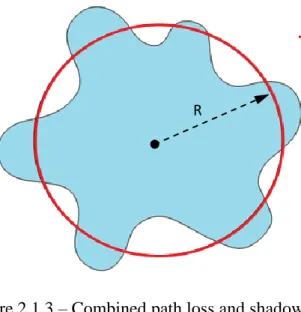
receiver. These obstacles attenuate the propagating signal power by absorbing, reflecting, diffracting or scattering. Shadowing occurs over tens or some hundred meters and is also seen as a part of large scale fading, which in fact can be also categorized as middle-scale fading. Variation of the signal due to path loss occurs over very large distances, 100 m up to 1 km. However in the case of shadowing the variation occurs over distances proportional to the length of the obstructing object, typically in the order of building dimensions, 10 m up to 100 meters. Especially in cellular system design, when modeling the coverage area of a cell, path loss and a shadowing model is combined. Figure 2.1.3 depicts contours of constant received power due to path loss plus random or average shadowing.
Figure 2.1.3 – Combined path loss and shadowing.
The second group is called small-scale models that focus on the instantaneous behavior of the received signal. These models are called small scale because here the issue is the variations of instantaneous signal strength over very short time intervals or very short distances with respect to the wave length. Moving the mobile the distance of one wavelength may cause a variation in the received signal strength of up to 40 dB. Unlike the predictions in large scale models, the variation of the signal is not a gradual decrease. The speed of motion is also a parameter that effects the variation in the signal level. Especially in urban and heavily populated areas the received signal is the vector sum of the scattered, reflected and diffracted signals which arrive at the receiving point from various directions with various propagation mechanisms. These propagation mechanisms cause rapid and dramatic variations for the resultant received signal as the mobile moves a few wavelengths.
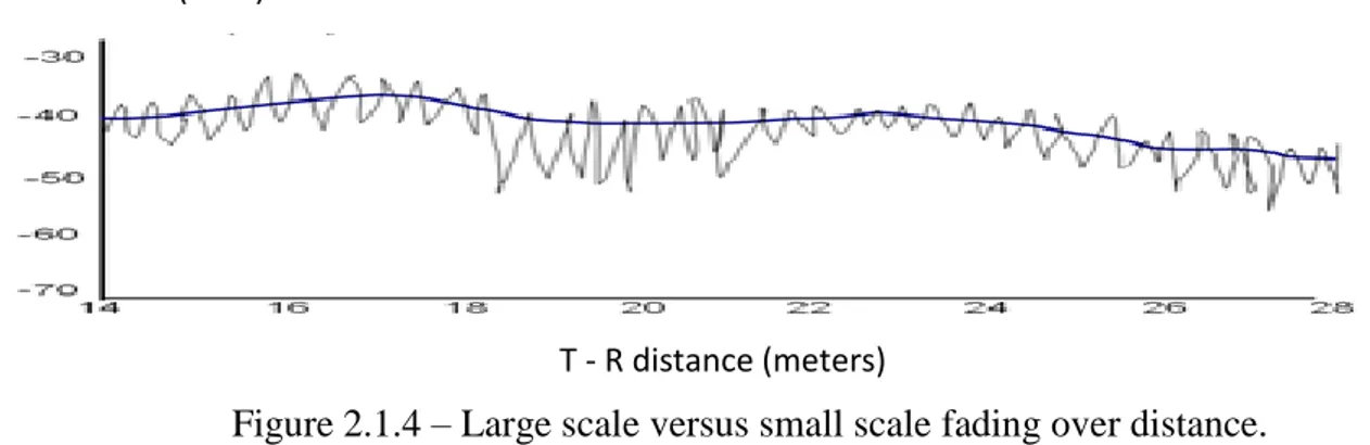
It is also important to point out that the dominant propagation mechanism in small scale fading is not reflection but scattering. Due to the fact that the phases of the received signals are random, the sum of all these different components behaves like noise. In this case the Rayleigh fading model can be used. To overcome the fading, MIMO technology may be used to achieve diversity by combining signals. The signal attenuation can be either Rayleigh distributed or Rician distributed, depending on whether there is line of sight (LOS) or not. If there are a lot of scattered components but no LOS then the attenuation coefficient can be effectively modeled as Rayleigh distributed. If there is LOS then one can apply the Rician distribution. The small scale fading model is a short term model and the severe signal fluctuations usually happen around a slowly varying mean. Figure 2.1.4 illustrates the received power variations with distance for both types of fading.
Path loss + random shadowing Path loss + average shadowing
Figure 2.1.4 – Large scale versus small scale fading over distance.
Figure 2.1.5 illustrates the received signal strength variations in large and small scale models over time. Red and green curves represent the means in large and small scale fading, respectively. One can imagine that a person is holding a power-meter and taking signal strength measurements while moving along. On top in Figure 2.1.5 large scale fading is plotted while small scale fading is plotted at the bottom. Both fadings have slowly varying means. But one can also see that even the mean variations in the small scale fading are faster than in the large scale fading.
Figure 2.1.5 – Large scale versus small scale fading over time.
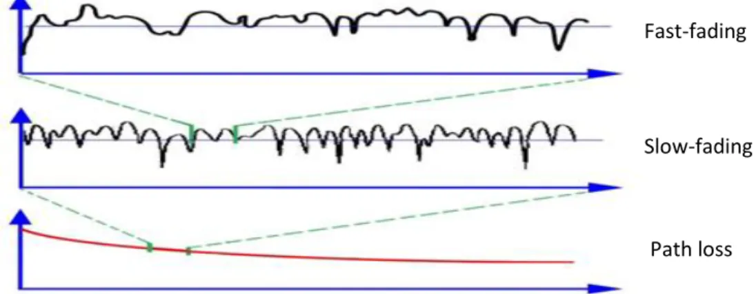
Figure 2.1.6 illustrates the same scenario and depicts the relation between the received signal strength and the distance from the transmitter. If one takes a small segment from the path loss curve and magnifies it, as in the middle figure, one finds a slow-fading (shadowing) curve. However if one again magnifies a small section from the slow-fading curve and analyzes it in detail one finds a fast-fading (short-term fading) curve. So fading can be subdivided into two additional types of fading which of course have different mathematical descriptions.
Received Power (dBm)
T - R distance (meters)
Received Power strength (dBm)
Figure 2.1.6 – Path loss vs. Slow-fading vs. Fast-fading.
As the mobile user moves away from the transmitter, measurements with a power-meter probably yield a graphic similar to Figure 2.1.4 with a decreasing trend with fluctuations around the mean. If the same user repeats this experiment he will get a similar but not the same curve. Figure 2.1.7 also shows the received power variations of the overall signal and its components as the receiver moves away from the transmitter. The horizontal axis corresponds to the T-R distance and the perpendicular axis corresponds to the power in dB.
Figure 2.1.7 – Components of Overall Signal as a function of distance.
Fast-fading
Slow-fading
Path loss Received Signal Strength (dB)
2.2.2 Path loss Models due to Propagation Mechanisms 2.2.2.a Path loss due to reflection and the Two Ray model
Reflection of an electromagnetic wave occurs when it impinges upon an object with different electrical properties and very large dimensions compared to the wavelength [4]. The wave impinging upon a new medium is partially transmitted into the second medium and partially reflected back to the first medium. If the second medium is perfectly dielectric there is no energy loss during reflection. If one assumes a second medium which is a perfect conductor, all the incident energy is reflected back into the first medium without any loss. When the first medium is free space and the permeabilities of two media are 12, the electric field intensity of the reflected and the transmitted waves are related by the simplified Reflection
Coefficient [4, 5]: | | j r i E e E , (2.2.1) and, 2 2 2 2 sin cos
for vertical polarization
sin cos
sin cos
for horizontal polarization
sin cos r i r i v r i r i i r i h i r i (2.2.2) where, i
is the grazing angle as shown in Figure 2.2.1 and r is the complex dielectric constant of the ground.
Reflection causes multipath effects. It may also be used (passive metallic reflectors) for covering areas which are normally not covered. To know the electrical properties of the reflector surface is important when it comes to modeling.
Materials in rooms that cause reflections are made out of dielectrics (walls, tables etc.). There are also nearly perfect conductors such as metal frames in the windows that form perfect reflectors.
At this point it is important to note that the statistical models begin to fail above 10 GHz. Above 10 GHz one has to search for a deterministic model in terms of rays.
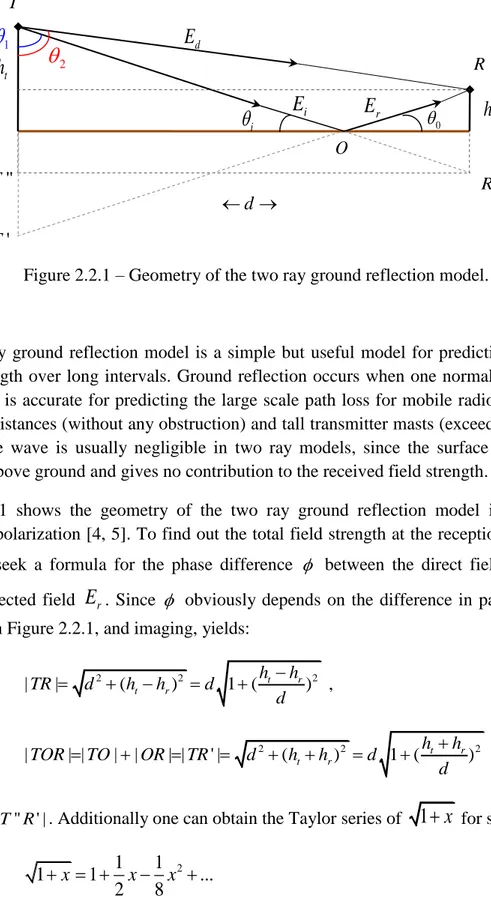
Figure 2.2.1 – Geometry of the two ray ground reflection model.
The two ray ground reflection model is a simple but useful model for predicting large scale signal strength over long intervals. Ground reflection occurs when one normally has a LOS. This model is accurate for predicting the large scale path loss for mobile radio systems with large T-R distances (without any obstruction) and tall transmitter masts (exceeding 50 m) [4]. The surface wave is usually negligible in two ray models, since the surface wave extends about 1 λ above ground and gives no contribution to the received field strength.
Figure 2.2.1 shows the geometry of the two ray ground reflection model in the case of horizontal polarization [4, 5]. To find out the total field strength at the reception point R one must first seek a formula for the phase difference between the direct field
E
d and the ground reflected fieldE
r. Since obviously depends on the difference in path lengths the geometry in Figure 2.2.1, and imaging, yields:2 2 2 | | ( ) 1 ( t r) t r h h TR d h h d d , (2.2.3) 2 2 2 | | | | | | | ' | ( ) 1 ( t r) t r h h TOR TO OR TR d h h d d , (2.2.4) where d = |T R'' ' |.Additionally one can obtain the Taylor series of
1 x
for small x as,2 1 1 1 ... 2 8 1 x x x (2.2.5) For x<<1 one has,
i
E
dE
rE
T R ' R th
rh
O i
0 2
1
d '' T'
T
1/2 (1 ) 1 1 2 x x . (2.2.6) In this case, 2 (ht hr) x d or (ht hr)2 x d and
d
h
th
r . (2.2.7) The difference in length then can be written as,2 2 1 1 2 1 ( ) (1 ( ) ) 2 2 t r t r t r h h h h h h d d d d d . (2.2.8) The phase difference then becomes [6],
2 4 h ht r d d
. (2.2.9) Here is the phase delay due to the path length difference. But there is also another phase delay which occurs at the point of reflection O. The reflection coefficient,| |
e
j
, (2.2.10) changes the amplitude and the phase of the impinging wave on reflection.In the case of vertical polarization, for very large distances, the vertical vector components
d
E
andE
i becomes almost the same. It can be seen from the geometry that,1 sin | ' | d TR and sin 2 | | d TR . (2.2.11) Assuming
i
0
for very large distances one can see that |TR| | TOR| andsin
1
sin
2 which results in equal vertical components of the electric fields in the z direction. In the case of horizontal polarization, the incident and reflected electric field are also assumed to remain the same, independent of the grazing angle.The equality of the angles
i and 0 can be derived by using boundary conditions from Maxwell’s equations in a dielectric. In the case of vertical and horizontal polarization, when0 ( =180 )
i
, the reflected waveE
r is assumed to be 180° out of phase but equal in magnitude withE
i. The reflection then gives a phase shift | | j 1 j 1e e
when
0
iTotal electric field strength at the point R is, (1 j ) (1 j ) tot d r d d E E E E e E e , (2.2.12) (1 cos sin ) tot d E E j . (2.2.13) For the amplitude one can write,
2 2 2 2
|Etot| | Ed | {(1 cos )
(sin ) } ,
(2.2.14) which simplifies to,
2 2 2 | | 4 | | sin 2 tot d E E
. (2.2.15) Thus, the received signal can be written as,2 | | 2 | | sin( t r) tot d h h E E d
. (2.2.16) The average power density for the direct path was introduced as,2 2 | | ( ) 4 rms t t E PG t d w , (2.2.17) so for the direct wave,
2 4 d PtGt E d , (2.2.18) and in free space,
30 t t d PG E d . (2.2.19) The resultant field can then be written as,
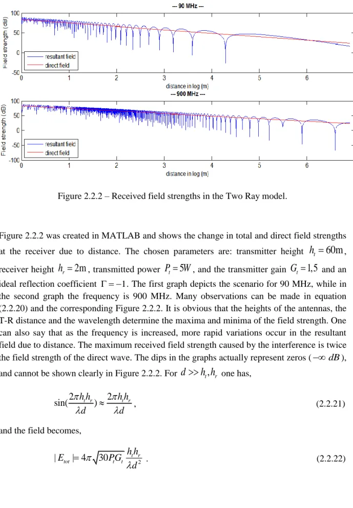
30 2 | | 2 t t sin( t r) tot PG h h E d d . (2.2.20)
Figure 2.2.2 – Received field strengths in the Two Ray model.
Figure 2.2.2 was created in MATLAB and shows the change in total and direct field strengths at the receiver due to distance. The chosen parameters are: transmitter height
h
t
60m
,receiver height
h
r
2m
, transmitted powerP
t
5
W
, and the transmitter gainG
t
1,5
and anideal reflection coefficient 1. The first graph depicts the scenario for 90 MHz, while in the second graph the frequency is 900 MHz. Many observations can be made in equation (2.2.20) and the corresponding Figure 2.2.2. It is obvious that the heights of the antennas, the T-R distance and the wavelength determine the maxima and minima of the field strength. One can also say that as the frequency is increased, more rapid variations occur in the resultant field due to distance. The maximum received field strength caused by the interference is twice the field strength of the direct wave. The dips in the graphs actually represent zeros ( dB), and cannot be shown clearly in Figure 2.2.2. For
d
h h
t,
r one has,2 2
sin( h ht r) h ht r
d d
, (2.2.21)and the field becomes,
2 | | 4 30 t r tot t t h h E PG d
. (2.2.22)At this point an expression for the total average received power can be derived as follows: 2 2 2 2 2 4 2 r (4 ) 30 | | P 120 4 t r t t r er h h PG E d G A , (2.2.23) which simplifies to the following equation:
2 2 r 4 P t r t t r h h PG G d . (2.2.24) Equation (2.2.24) shows that for very large distances the resultant field strength falls faster than the direct field. Independent of frequency, the received power decays as 14
d [4]. This is good for avoiding interference in cellular systems. This simplistic but realistic model can hold good for mobile application at GSM frequencies. The model is applicable in LOS scenarios but LOS is seldom found as one moves very large distances away from the transmitter. Since the antenna gains are fixed, the way to adjust the signal is usually to change the antenna heights.
2.2.2.b Path loss due to diffraction
Geometrical optics doesn’t include the field in the shadow of an obstruction, since it is based on rays. However, to some agree the E-M waves can propagate into the geometrical shadow depending on the wavelength, shape, height and location of the obstruction. Especially in the case of deterministic modeling diffraction models should be used.
A knife-edge geometry, depicted in Figure 2.2.3, is a special simplistic case of diffraction where there is a single obstacle which is assumed to be extremely sharp so that no significant reflections can occur. It has infinite width along z-axis (perpendicular to the page). Assuming diffraction without any transverse effects one may reduce the scenario to 2-D. It is also assumed that the obstacle in Figure 2.2.3 absorbs all the upcoming waves below its tip [4].
Figure 2.2.3 – Knife-edge geometry for a single obstacle.
h T h' 1
'
d
1d
R 2'
d
1d
1d
2d
According to the knife-edge diffraction geometry in Figure 2.2.3 the path difference can be found as follows where h' ',d d1 2' [4, 5]:
2 2 2 2
1' ' 2' ' ( 1' 2')
d h d h d d
, (2.2.25) which can also be written as,
2 2 1 2 1 2 1 2 ' ' ' 1 ( ) ' 1 ( ) ( ' ') ' ' h h d d d d d d , (2.2.26) and the approximate path length is,
2 2 1 2 1 2 1 2 1 ' 1 ' '(1 ( ) ) '(1 ( ) ) ( ' ') 2 ' 2 ' h h d d d d d d , (2.2.27) 2 1 2 1 2 ' ( ' ') . 2 ' ' h d d d d (2.2.28)
Since in practice hd d1, 2, the equations can be approximated in terms of distances parallel to and normal to the ground, one has, h h d ', 1d1' and d2 d2'. Hence the phase difference becomes, 2 1 2 1 2 2 h (d d ) d d . (2.2.29) Assuming that , and , the pitch angle, are very small,
1 2 1 2 ' ' tan tan '( ) ' ' d d h d d , (2.2.30) so that approximately, in radians,
1 2 1 2 (d d ) h d d . (2.2.31) It is important to mention the Fresnel ellipsoids since obstructions that penetrate the first Fresnel zone play a significant role in diffraction loss. If the propagating waves are considered to bend at every point between T and R then the same path length forms an ellipsoid. A Fresnel ellipsoid is a surface where the excessive path length is constant and has values,
2 n
, (2.2.32)
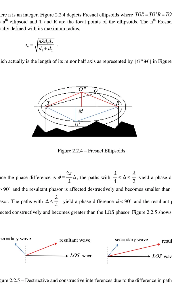
where n is an integer. Figure 2.2.4 depicts Fresnel ellipsoids where TOR TO R TO R ' '' form the nth ellipsoid and T and R are the focal points of the ellipsoids. The nth Fresnel zone is usually defined with its maximum radius,
1 2 1 2 n n d d r d d , (2.2.33) which actually is the length of its minor half axis as represented by |O M'' | in Figure 2.2.4.
Figure 2.2.4 – Fresnel Ellipsoids.
Since the phase difference is
2
, the paths with
4 2
yield a phase difference
90
and the resultant phasor is affected destructively and becomes smaller than the LOS phasor. The paths with
4
yield a phase difference 90 and the resultant phasor is affected constructively and becomes greater than the LOS phasor. Figure 2.2.5 shows this,
Figure 2.2.5 – Destructive and constructive interferences due to the difference in path lengths. resultant wave resultant wave
LOS wave LOS wave
secondary wave secondary wave T O R ' O '' O M
Often the Fresnel-Kirchhoff diffraction parameter is used as a normalized phase difference, 1 2 1 2 1 2 1 2 2( ) 2 ( ) d d d d h d d d d , (2.2.34) or simply, 2 v . (2.2.35) By applying Huygens principle to radio waves, one can predict the received signal in the shadow region as the phasor sum of the electric field components of all secondary wavelets from the obstacles [7]. Since Huygens principle assumes all these incoming and outgoing wavelets to be spherical, one should use Fresnel diffraction.
It is important to emphasize that in Fraunhofer diffraction the incoming and outgoing wave-fronts are assumed to be planar and the propagation paths after obstruction are assumed to be parallel. So the phase differences between each consecutive element of the wave front increases linearly which results in constant phase differences between consecutive elements of the wave front. Also the paths taken by the waves are considered to be the same for very large distances, again because of the parallelism, which results in equal amplitudes at a point of observation. Thus the phasors of these elements form an arc of a circle at a point of observation.
In Fresnel diffraction the outgoing wave-fronts are considered to be composed of tiny spherical wavelets and the propagating wavelets’ rays from the obstruction axis to the point of observation are not parallel. The phase differences do not increase linearly between two consecutive elements.
Figure 2.2.6 – Huygen’s principle and Fresnel diffraction geometry.
P x ' y P 1
h
2h
3h
d 3d
h yIn Figure 2.2.6, at point P the phase differences of the wavelets from the elements at , 1
, , ,...,
2 3 nh h h
h
, whereh
2
h
1h
3h
2...
h
nh
n1, is directly related to the path differences, 2 1 ( ) n n d h h d d , (2.2.36) which can be written in the form,2 1 ( 1 ( n ) 1) n h h d d d . (2.2.37) Binomial approximation for
h
n
d
path yields,2 2 1 1 1 ( ) 1 1 2 2 n n n h h h h d d d d , (2.2.38) and the phase difference for the nth element is approximately,
2 1 ( n ) n h h d . (2.2.39) This shows that the linear increase in height causes a quadratic increase in phase difference. If one marks the consecutive points with a constant phase increment ' C, i.e. the points
1 2 ' , ' ... 'n
h h h where
'
'
1'
2
'
3'
2
...
'
n
'
n1, one can write the following expression: 2 2 1 1 1 1 ' ' ' [( ' ) ( ' ) ] 2 n n h n h h n h C d
. (2.2.40) To satisfy the equation (2.2.40), one can see that h'2h'1h'3h'2 ... h'nh'n1. This means that for a linear step in phase, the step in height must decrease with n. Here the height difference h'nh'n1 is proportional to the radius and the effect of each wavelet at the observation point. Hence, the contribution of each wavelet reduces for a linear increase in phase difference [7]. At a point of observation, phasors of these elements form a curve called the Cornu spiral.In Figure 2.2.6 the incident plane wave can be defined as,
0
( , ) jkx inc
E x y E e . (2.2.41) Applying the Kirchhoff integral and Huygens’s principle to the geometry in Figure 2.2.6 for the region x0, the total electric can be written as [8, 16],
(2.2.42) where, 2 x . (2.2.43) and y is the axis of the point P in Figure 2.2.6. The integral can be written in terms of
Fresnel Integrals with the cosine integral, 2 0 ( ) cos( ) 2 v C v
u du , (2.2.44) and the sine integral,2 0 ( ) sin( ) 2 v S v
u du , (2.2.45) and the Fresnel-Kirchhoff parameter,' v y . (2.2.46) Thus, 2 ( /2) 0 ( ) ( ) v j u C v jS v
e du . (2.2.47) The asymptotic expansions for v1yield,2 1 1 ( ) cos( ) 2 2 C v v v
, (2.2.48) 2 1 1 ( ) sin( ) 2 2 S v v v
. (2.2.49) The limit, 1 1 lim[ ( ) ( )] 2 2 v C v jS v j , (2.2.50) yields, 2 ( /2) 0 1 (1 ) 2 j u e du j
, (2.2.51) 2 ( /4) ( /2) 0 ( , ) , 2 j kx j u tot y E e E x y e du
and the expression for the total field can be rewritten as [8], ( /4) 0 1 1 ( , ) [ ( ) ( )] 2 2 2 j kx tot E e E x y j C y jS y . (2.2.52)
To illustrate the amplitude changes due to height for a fixed distance x from the edge, the absolute value of the conjugate is of interest
1 1
[ ( ) ( )]
2 2
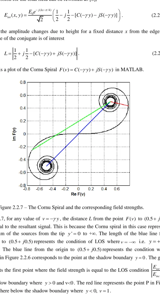
L j C y jS y . (2.2.53) Figure 2.2.7 is a plot of the Cornu Spiral F v( )C(y) jS(y) in MATLAB.
Figure 2.2.7 – The Cornu Spiral and the corresponding field strengths.
In Figure 2.2.7, for any value of v y, the distance L from the point F v( ) to (0.5 j0.5)
is proportional to the resultant signal. This is because the Cornu spiral in this case represents the vector sum of the sources from the tip y'0 to +∞. The length of the blue line from
( 0.5 j0.5) to (0.5 j0.5)represents the condition of LOS wherev i.e. y in
Figure 2.2.6. The blue line from the origin to (0.5 j0.5)represents the condition where 0
v which in Figure 2.2.6 corresponds to the point at the shadow boundary y0. The green line represents the first point where the field strength is equal to the LOS condition tot 1
inc
E
E
over the shadow boundary where y0 and v<0. The red line represents the point P in Figure 2.2.6, somewhere below the shadow boundary where y0, v1.
The total field relative to the incident field is, 4 1 1 [ ( ) ( )] 2 2 2 j tot inc E e j C y jS y E , (2.2.54)
and using the identity,
4 1 1 2 2 j e j , (2.2.55) it becomes, [1 ( ) ( )] [ ( ) ( )] 2 tot inc E C v S v j S v C v E . (2.2.56) Figure 2.2.8 represents the plots of the absolute values of the total field strengths relative to the direct field tot
inc
E
E both in linear and decibel scales due to the parameter v in MATLAB. Large positive values of v correspond to deep shadow.
Figure 2.2.8 – Relative field strength tot inc
E
E due to the parameter v in linear and dB scales. The terms with Fresnel integrals in equation (2.2.56) makes the computation difficult. Therefore, when predicting the knife-edge diffraction loss, equation (2.2.56) can be approximated by the expression given by Recommendation ITU [8] for v 0.7,
2
10 10
20log tot ( ) 6.9 20log [ ( 0.1) 1 0.1] [dB]
inc
E
J v v v
Approximations for tot inc
E
E in dB are also given by Lee [4],
10 0.95 10 ( ) 0 -1 ( ) 20 log (0.5 0.62 ) -1 0 ( ) 20 log (0.5 v) J v v J v v v J v e 2 10 10 0 1 ( ) 20 log (0.4 0.1184 (0.38 0.1 ) 1 2.4 0.225 ( ) 20 log ( ) >2.4 v J v v v J v v v
Figure 2.2.8 shows the diffraction loss due to height for a fixed frequency. However if the frequency is increased for the same scenario the ratio tot
inc
E
E decreases more quickly. Figure 2.2.9 shows the diffraction losses for 1 GHz and 4 GHz at a point of observation x=100 m and -15<y<15 meters. According to the figure, a higher frequency produces a more distinct shadow.
Figure 2.2.9 - Relative field strength tot inc
E
E for 1 GHz and 4 GHz.
The first Fresnel zone is crucial for diffraction loss. If the frequency is increased for an obstructed path, due to equation (2.2.33), the first zone gets narrower and the diffraction loss may be reduced. However, as can be understood from Figure 2.2.9 and considering the geometry in Figure 2.2.6, at higher frequency, for a fixed observation point x, moving the point in -y direction or increasing the height of obstruction causes diffraction loss to happen more quickly. The related parameters are,
1 2 1 2 2 2(d d ) v y y h d d x . (2.2.59) (2.2.58)
3. PROPAGATION MODELS
3.1 PROPAGATION MODELS FOR RURAL AREAS
3.1.1 Deterministic Multiple Edge Diffraction Models
When predicting the path loss between two fixed stations for large distances, the path profile between the stations is often reduced to single knife edges since the wavelength is short compared to the size of obstacles such as hills. The total path loss is then the free space loss plus the predicted obstruction loss of the two-dimensional multiple edge diffraction model. For multiple knife-edge geometry the waves incident on the edges will not be plane after the first edge and the Fresnel integral should be evaluated consecutively for each edge to obtain a deterministic loss prediction. Hence, for n edges an n-dimensional Fresnel integral must be evaluated. This is very difficult to implement. A method with extreme accuracy for the attenuation of electromagnetic waves by multiple edges is given by L. E. Vogler. Starting from Furutsu’s generalized residue series formulation for electromagnetic waves over a sequence of smooth cylindrical obstacles, Vogler derived an attenuation function for multiple knife edges using Fresnel-Kirchhoff theory [12]. In his derivation he replaces the residue series in Furutsu’s method with a contour integral since the series converges slowly in the case of a grazing incidence. Vogler obtains an N-dimensional integral
I
N by considering the cylindrical surfaces with zero that correspond to N multiple knife-edge geometry and describesC
N as the spreading loss factor over the propagation path in his formula [9]. The attenuationA
N, which is the ratio of total loss relative to the free space loss for N edges (see Figure 3.1.1), is given as follows [9, 10]:/2 (dB) N N N N N A C
e I , (3.1.1) where, 1 2 2 3 1 2 ... ( ) n T N N m m m d d d d C d d
, (3.1.2) 2 1 1 1 2 1 ... ... N m m N N f x N N x x I e dx dx
, (3.1.3) for N 2; andC
N
1
for N 1 whered
T
d
1...
d
n1 and,1 1 2 1 1 ( , ,..., ) ( )( ) , N N m m m m m f x x x x x
(3.1.4)for N 2; and f 0 for N 1 . 2 1 N N m
, (3.1.5) 2 1 1 2 ( )( ) m m m m m m m d d d d d d , (3.1.6) 1 1 1 2( ) m m m m m m m jkd d r d d , (3.1.7)where r1 is the radius of the first Fresnel zone.
Figure 3.1.1 depicts the geometry in Vogler’s method where the given 1, ,3 n are taken
positive since h1h h h2, > and >3 4 hn hn1 and
2 is taken negative since h2h3. d is the ndistance between (n1) and nth th edges.
Figure 3.1.1 – Multiple edge geometry for Vogler’s integral method.
Vogler transforms the multiple integral
I
N in equation (3.1.3) into an infinite summation1 m m I
which can be computed numerically. The simplified solution for the attenuationA
N becomes, /2 1 , N N N N m m A C e I
(3.1.8) where, 0 0 1 1 1 0 1 1 1 0 0 2 ( , ) (2, , ) , m m m m m m I I m m C m m
(3.1.9) 1
3
n 2
1d
1
2d
1
3d
1
1 nd
1
0 h h1 h2 h3 hn hn10 ( )! ( , , ) ( , ) ( 1, , ) , ( )! j j i N L N L i k i C N L j k I k i C N L i j j i
(3.1.10) with the repeated integrals of the error function,2 1 1 ( , ) ( ) , ! n x I n x e dx n
(3.1.11) and, 2 2 3 3 1 3 1 2 ( 1, , ) ( )! mN ( , ) ( , ) , N N N N N N N N C N m m m
I m
I m
(3.1.12) where the notations are given [9],1 2 0 , , 2 2, N 4 1, m , m 0 when k N-1 N L N L N L N k i m j m k m L N m
3.1.2 Approximate Multiple Edge Diffraction Models
Because of its computational rigor, Vogler’s method is usually used when comparing the accuracy of approximate methods. Commonly used approximate methods are the Bullington, Epstein-Petersen, Japanese, Deygout, and Giovanelli methods [10].
3.1.2.a The Bullington method
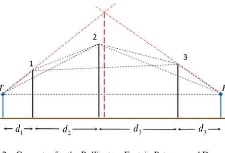
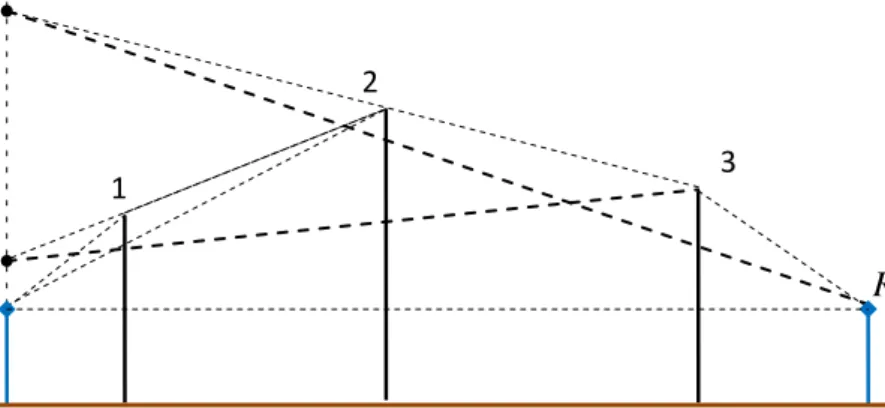
The terrain profile must be reduced to knife edges before the Bullington method is implemented. To compute the diffraction loss, an equivalent knife edge is determined by reducing all knife edges to a single knife edge. To determine the equivalent knife edge, two lines are drawn joining transmitter and receiver to with respective dominant edges which has the greatest angle of elevation. The intersection point of these two lines is the top of the equivalent knife edge and the diffraction loss is calculated as if it were the only obstacle [7]. In Figure 3.1.2 the dashed red lines depicts the Bullington geometry.
Figure 3.1.2 – Geometry for the Bullington, Epstein Petersen and Deygout methods.
3.1.2.b The Epstein-Petersen method
Here, attenuation due to each obstacle is calculated and summed to find the total diffraction loss. For instance, in Figure 3.1.2 the geometries of each triangle T12, 123 and 23R are taken as a simple knife-edge geometry and diffraction losses are computed individually and summed. For each case the obstruction lengths above the lines T2, 13 and 2R can be found by using simple geometrical laws. This method results in large errors when the obstacles are close [11]. In this case the Millington correction is added to the original loss,
10
' 20log (cosec )
L
, (3.1.14) where is the spacing parameter for the thn and (n1)th edges. The spacing parameter is found from the formula [11],
1/2 1 1 2 1 1 2 ( )( ) cosec . ( ) n n n n n n n n d d d d d d d d (3.1.15)
The Epstein-Petersen method calculates the diffraction loss for N successive knife edges and can be written as [12], 1 ( ) | ( ) | N epstein i i L N L v
, (3.1.16) where, 2 1 3 T R 1d
1
2d
1
3d
1
3d
1
2 2 1 ( ) 2 i j t i v j L v e dt
, (3.1.17)is the diffraction loss for the th
i knife edge. Since Vogler’s simplified attenuation function is,
vogler 0 1 ( ) ( ) | | 2 N N m m L N C I
, (3.1.18)then for m=0 the Epstein-Petersen loss can be described in terms of Vogler’s loss as, vogler( ) | 0 ( ) m epstein N L N L N C , (3.1.19)
which shows that Epstein-Petersen method turns out to be a first order approximation of Vogler’s method and underestimates the
C
N spreading loss factor.3.1.2.c The Japanese method
From the top of each obstruction a horizon ray is drawn which also passes from the top of the previous obstruction. The intersection point of this horizon ray with the plane of the terminal is then seen as the effective source. For instance, in Figure 3.1.3 the diffraction losses from each obstruction are calculated due to the geometries of 12, T'23 and T''3RT . The sum of these gives the total diffraction loss [11]. Actually this method is equivalent to the Epstein-Petersen method plus the Millington correction given in equation (3.1.14).
Figure 3.1.3 – Geometry for the Japanese method.
'' T 2 1 3 R ' T T
3.1.2.d The Deygout method
First the v parameter is calculated for each obstacle as if there were no other diffracting obstacles. Secondly, the dominant edge which has the maximum v parameter is determined and the diffraction loss is calculated as if it were the only edge. The dominant edge now becomes the terminal point of two sections divided by it. Then the process is repeated recursively by finding out the maximum v parameter and determining loss until all edges are considered. The total diffraction loss is then the sum of all these losses. For the geometry in Figure 3.1.2 the total excess loss L in single edge diffraction terms can be computed by the following expressions [13]: 1 2 3
(dB)
totalL
L
L
L
(3.1.20) where20log |
|
i iL
A
(3.1.21) 2 2 1 i i x i A e e dx
(3.1.22)where is calculated as in Vogler's method.i
If the edges are too many or too close, the Deygout method overestimates the path loss. In these cases Causebrook introduces a correction which reduces the overestimated path loss as follows: 1 2
(6
1 2)cos
1 3(6
1 3)cos
3,
totalL
L
L
L
L
L
L
L
(3.1.23) where, 1 3 4 1 1 2 2 3 4 ( ) cos , ( )( ) d d d d d d d d 4 1 2 3 1 2 3 3 4 ( ) cos . ( )( ) d d d d d d d d 3.1.2.e The Giovanelli method
Figure 3.1.4 relates to this method. As in the Deygout method firstly the dominant edge is determined due to the v parameter. Edge M represents the dominant edge. Then a reference point R’ is found by projecting a line on to the RR’’ plane which starts from M and passes through the adjacent edge N. The loss due to the v parameter for the TMR’ geometry is then (3.1.24)
calculated by obtaining the excessive effective height [10, 13]. The effective height for edge M which is the excess height above TR’ is,
1 1 1 1 2 3 '' d H , h h d d d (3.1.25) where, 2 3
H
h
md
and 2 1 2 . h h m d (3.1.26)So the loss from edge M can be written as a function of the TMR’ geometry parameters as,
1 2 3 1
( ,
,
'') .
M
L
f d d
d h h
(3.1.27)
After computing the loss from the dominant edge the dominant edge now becomes the terminal point for two sections divided by it, as in the Deygout method. The same process is applied to the remaining secondary edge N. The effective height for edge N which is the excess height above MR is,
3 1 2 2 2 3 ' d h . h h d d (3.1.28)
So the loss from edge N can be written as a function of the MNR parameters as,
2 3 2
( , ,
') .
N
L
f d d h h
(3.1.29)
The total loss can then be written as,
.
total M N
L
L
L
(3.1.30)
For n edges this process is repeated until there are no edges left to be considered.
Figure 3.1.4 – Geometry for the Giovanelli method.
'' R M N ' R 1
![Figure 3.1.5 depicts a slope UTD diffraction geometry with a wedge, where TT ' is the incident shadow boundary and T T R R ' is the reflection boundary [17]](https://thumb-eu.123doks.com/thumbv2/5dokorg/5475465.142495/40.892.158.631.317.1186/figure-depicts-diffraction-geometry-incident-boundary-reflection-boundary.webp)
