C851
.C47
no.
35
ARCHIVE
ISSN No. 0737-5352-35AEROSOL HYGROSCOPICITY AND VISIBILITY 'ESTIMATES
IN THE GREAT SMOKY MOUNTAINS NATIONAL PARK
Jenny L. Hand and Sonia M. Kreidenweis
Department of Atmospheric Science Colorado State University
Fort Collins, CO
Funding Agency:
National Park Service # 1443-CAOOO1-920006, AMD#5/SUB#3
June, 1997
I
O;j 1999
AEROSOL HYGROSCOPICITY AND VISmILITY ESTIMATES IN THE GREAT SMOKY MOUNTAINS NATIONAL PARK
Jenny L. Hand
Sonia M. Kreidenweis Department of Atmospheric Science
Colorado State University Fort Collins, CO
ABSTRACf
Summertime visibility in the National Parks in the Eastern United States is often very poor, due to high particulate mass concentrations and high relative humidities. As a part of the Southeastern Aerosol and Visibility Study (SEA VS) in the Great Smoky
Mountains National Park during the summer of 1995, aerosol size distributions (Dp = 0.1-3 J.1lIl) were measured with an Active Scattering Aerosol Spectrometer (ASASP-X). A
relative humidity (RH) controlled inlet allowed for both dry and humidified measurements. The objective of this experiment was to examine the aerosol size distribution and its
variation with RH to characterize its effect on visibility in the region.
The AS ASP-X was calibrated with polystyrene latex spheres (PSL) (m = 1.588), however, the instrument response was sensitive to the refractive index of the measured particles, which was typically much lower than that of PSL. An inversion technique accounting for varying particle real refractive index was developed to invert ASASP-X data to particle size.
Dry (RH
<
15%) particle refractive indices were calculated using the partial molarrefractive index method and 12-hour fine aerosol
«
2.5 J.1lIl) chemical compositions from the National Park Service Interagency Monitoring of Protected Visual Environments (IMPROVE) filter samples. A study average dry refractive index of m=
1.49±
0.02 was determined. The dry aerosol number distributions inverted using the scaling method were fit with single mode lognormal curves, resulting in dry accumulation mode size parameters. A study average total volume concentration of 7±
5 J.1m3 cm-3 was determined, with a maximum value of 26 J.1m3 cm-3• The large variability was due to extremes inmeteorological situations occurring during the study. The study average volume median diameter was 0.18
±
0.03 J.1m, with an average geometric standard deviation of 1.45±
0.06.A newly-developed iteration method was used to determine wet refractive indices, wet accumulation mode volume concentrations and water mass concentrations as a function of relative humidity. Theoretical predictions of water mass concentrations were determined using a chemical equilibrium model assuming only ammonium and sulfate were
hygroscopic. Comparisons of predicted and experimental water mass showed agreement within experimental uncertainties.
To examine the effects of particles on visibility, particle light scattering coefficients,
b sp' were calculated with derived size parameters, refractive index and Mie theory. Dry
scattering agreed well with nephelometer measurements made at SEA VS, with an average
hsp of 0.0406 lan-I. Estimates of particle light scattering growth (bib) were determined from ratios of wet and dry light scattering coefficients, and also agreed with nephelometer results.
The new inversion techniques were compared to earlier, simpler methods which ignored variations in aerosol chemical composition. The simpler method yielded smaller mean diameters, however, hygroscopicity estimates were comparable to those derived using daily varying chemical composition. This suggests that although the aerosol
chemical composition is needed to determine aerosol size parameters, it may not be critical for deriving hygroscopicity (or other ratios of size parameters). This result may be specific to this study, as the variation in refractive index with RH assumed by previous models appears to be a good estimate for that observed during SEAVS.
ACKNOWLEDG:MENTS
We would like to thank the following people at CSU for their support of this work: Rodger Ames, Derek Day, Eli Sherman, and Brian Jesse.
Several people at the Air Quality Division of the National Park Service/CIRA also contributed to this work: William MaIm, Kirk Fuller, and Jim Sisler. To them we also express our gratitude.
Several people generously allowed us to use their computer programs in this work. Dr. Chris Pilinis of the University of Miami provided his EQun..m program for estimating water mass concentration. Dr. Alfred Wiedensohler at the Institute of Tropospheric Research in Leipzig, Germany, made Evan Whitby's DISTFIT lognormal fitting program available to use with our aerosol size distributions. Dr. Peter McMurry and Bill Dick from the University of Minnesota provided helpful suggestions in deriving a scaling technique for data inversion.
Jenny Hand expresses her appreciation to her advisor, Dr. Sonia Kreidenweis, for her enthusiasm and availability during the course of this work. My gratitude also goes to Dr. Jeff Collett and Dr. Marty Fettman who gave of their time and helpful suggestions as committee members. Appreciation should also be extended to the CSU Atmospheric Chemistry group (especially Debra Y. Harrington) for their helpful suggestions in the preparation of this thesis. I must extend my overwhelming gratitude to my family: Mike, Ruth, Sharon, Dolan, and Cory, without whose help I am certain I would not have finished on time. And of course, Teegan, who provided so much laughter.
This research was supported by the National Park Service under contract number 1443-CAOOO 1-920006, AMD#5ISUB#3
TABLE OF CONTENTS
ABSTRACT ... iii
ACKNOWLEDGMENTS ... v
TABLE OF CONTENTS ... vi
LIST OF TABLES ... viii
LIST OF FIGURES ... ix
CHAPTER 1. INTRODUCTION ... 1
1.1 Experimental Background.. . . .. 3
CHAPfER 2. OPTICAL PARTICLE COUNTER ... 6
2.1 Theory . . . .. 6
2.2 Calibration. . . .. 9
2.3 Detennination of Channel Diameter. . . .. 12
2.4 Diameter Scaling Method. . . .. .. 18
CHAPTER 3. DATA INVERSION AND RESULTS USING A RURAL AEROSOL MODEL OF REFRACTIVE INDEX ... 23
3.1 Lognonnal Size Distribution Function ... 24
3.2 Particle Hygroscopicity ... 28
3.3 Particle Light Scattering ... 32
3.4 Particle Light Scattering Growth Curve ... 35
CHAPfER 4. DRY REFRACTIVE INDEX AND CHEMICAL COMPOSmON ... 37
4.1 Partial Molar Refractive Index Method ... 37
4.2 Volume Weighted Refractive Index Method ... 39
4.3 Chemistry ... 39
4.3.1 Choices of Chemical Composition ... 43
4.4 Final Choices for Refractive Index ... 46
4.5 Complex Refractive Index ... 48
CHAPfER 5. DETERMINATION OF WET REFRACTIVE INDEX ... 52
5.1 Method ... 52
5.2 Sensitivity of Iteration on Input Values ... ~ ... 54
5.3 Experimental Water Mass ... 57
5.4 Theoretically Predicted Water Mass ... 58
CHAPfER 6. SEAVS RESULTS BASED ON DAILY VARYING CHEMICAL COMPOSmON ... 65
6.1 Accumulation Mode Dry Size Parameters for Non-Absorbing Aerosol ... 65
6.2 Particle Hygroscopicity ... 67
6.3 Particle Light Scattering ... 69
6.4 Particle Light Scattering Growth Curve ... 70
6.5 Absorbing Aerosols: 'The Effects of Including Elemental Carbon ... 71
CHAPTER 7. CONCLUSION ... 74
CHAPTER 8. FUTURE WORK ... 77
APPENDICES
A. Sensitivity Studies to Analysis Methods and Instrument Calibration ... 84
A.1. Sensitivity Studies to Lognormal Size Distribution Functions ... 85
A.l.l. Total Number Concentration ... 85
A.1.2. Accumulation Mode Volume Concentration ... 86
A.1.3. Volume Median Diameter ... 87
A.1.4. Geometric Standard Deviation ... 89
A.l.5. Particle Hygroscopicity ... 90
A.l.6. Experimental Uncertainty ... 91
A.2. Sensitivity to Instrument Calibration ... 94
A.2.1. Total Number Concentration ... 94
A.2.2. Accumulation Mode Volume Concentration ... 94
A.2.3. Volume Median Diameter ... 96
A.2.4. Number Median Diameter ... 96
A.2.5. Geometric Standard Deviation ... 98
A.2.6. Particle Light Scattering ... > • • • • • • • • • • • • • • • • • • • • • • • • • • • • • • • 98 A.2.7. Particle Hygroscopicity ... 99
B. Sensitivity Studies to Daily Varying and Complex Refractive Index ... 101
B.l. Sensitivity Studies to Daily Varying Refractive Index ... 101
B.l.l. Total Dry Number Concentration ... 101
B.1.2. Dry Accumulation Mode Volume Concentration ... 101
B.l.3. Dry Number Median Diameter ... 103
B.l.4. Dry Volume Median Diameter ... 103
B.l.5. Dry Geometric Standard Deviation ... 104
B.l.6. Particle Light Scattering ... 104
B.l.7. Particle Hygroscopicity ... 106
B.2. Sensitivity of the Effects of Elemental Carbon ... 107
LIST OF TABLES
CHAPTER 1
1.1 Meteorological Periods During SEA VS ... 5 CHAPTER 2
2.2.1 ASASP-X Relative Gains and Normalization Constants ... 12 2.3.1 Lower Channel Limit Scattering Response and Diameters ... 16 CHAPTER 3
3.1.1 Rural Aerosol Model Refractive Index and Relative Humidity ... 23 3.1.2 Dry Accumulation Mode Size Parameters Using a Rural Aerosol Model ... 28 CHAPTER 4
4.3.1 Physical Constants of Species Used in Refractive Index Calculations ... 44 CHAPTER 5
5.2.1 Dry Input Values for Sensitivity Study ... 56 5.2.2 Percent Change in Dry Mass Fraction ... 57 5.4.1 Percent Change in Water Mass Ratio ... 63 CHAPTER 6
LIST OF FIGURES
CHAPTER 1
1.1 Great Smoky Mountain National Park and Surrounding Areas ... 4
CHAPTER 2 2.1.1 Discriminator Level Voltages for the ASASP-X Size Ranges ... 7
2.1.2 Theoretical Response Functions for the AS ASP-X ... 8
2.2.1 Discriminator Level Voltages Normalized by Relative Gain ... 11
2.3.1 Mie Theoretical Response for m
=
1.588 ... 132.3.2 Mie Theoretical Response for m
=
1.530 ... 152.3.3 PSL Number Distribution ... 17
2.4.1 Collapsed Mie Response around m = 1.530 ... 19
2.4.2 Diameter Scaling Factor as a Function of Refractive Index ... 21
2.4.3 Scaled Diameters for Various Refractive Index ... 22
CHAPTER 3 3.1.1 Example Aerosol Volume Distribution ... 25
3.1.2 Example Aerosol Number Distribution ... 26
3.1.3 Dry Accumulation Mode Size Parameters for the Rural Aerosol Model ... 27
3.2.1 Hygroscopic Growth for the Ammoniated Sulfate System ... 29
3.2.2a Hygroscopic Growth Using Volume Median Diameter Ratios ... 31
3.2.2b Hygroscopic Growth Using Accumulation Mode Volume Ratios ... 31
3.3.1 Timelines of Particle Light Scattering ... 35
3.4.1 Estimates of Particle Light Scattering Growth for the Rural Aerosol Model ... 36
CHAPTER 4 4.3.1 IMPROVE Mass Concentration ... 41
4.3.2 Ammonium to Sulfate Molar Ratio ... 41
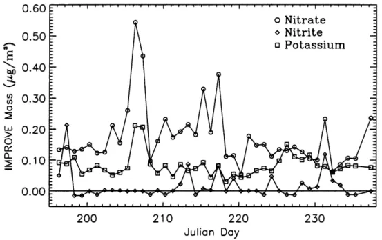
4.3.3 Nitrate, Nitrite and Potassium Mass Concentration ... 42
4.3.4 Soil Mass Concentration ... 42
4.3.5 Dry Soil Refractive Index ... 45
4.3.6 Refractive Index of Soil and Other Components ... 46
4.4.1 Soil Event Volume Distribution ... 47
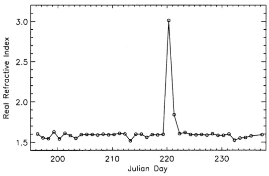
4.4.2 Dry Refractive Indices Used in the Data Inversion ... 49
4.5.1 Complex Refractive Indices ... 50
4.5.2 Mie Theoretical Scattering for Complex Refractive Indices ... 51
CHAPTER 5 5.1.1 Flow Chart of Wet Iteration Method ... 53
5.2.1 Solutions to Dry Mass Fraction Functional Equation ... 56
5.3.1a Water Mass as a Function of Relative Humidity ... 60
5.3.1b Water Mass as a Function of Wet Volume ... 60
5.3.1c Water Mass Fraction as a Function of Wet Density ... 60
5.3.1d Water Mass Fraction as a Function of Wet Refractive Index ... 60
5.4.1 IMPROVE and Accumulation Mode Dry Mass ... 61
5.4.2 Experimental and Theoretical Water Mass Ratio Comparisons ... 62
5.4.3a Theoretical Water Mass Ratio as a Function ofRH and ID ... 64
5.4.3b Experimental Water Mass Ratio as a Function ofRH and ID ... 64
CHAPTER 6 6.1 Dry Accumulation Mode Size Parameters for Varying Chemical Composition ... 66
6.2.1b Hygroscopic Growth Using Accumulation Mode Volume Ratios ... 68
6.2.2 Iterated Refractive Index as a Function of RH ... 69
6.3.1 Timelines of Particle Light Scattering ... 70
6.4.1 Estimates of Particle Light Scattering Growth for Varying Composition ... 71
6.5.1a Timelines of Particle Light Extinction and Scattering for Absorbing Aerosol ... 73
FIGURES IN APPENDICES APPENDIX A
A.1.1a. Comparisons of Dry Total Number Concentration ... 86
A.1.1b. Comparisons of Wet Total Number Concentration ... 86
A.1.2a. Comparisons of Dry Accumulation Mode Volume Concentration ... 87
A.1.2b. Comparisons of Wet Accumulation Mode Volume Concentration ... 87
A.1.3.1a. Comparisons of Dry Volume Median Diameters ... 88
A.1.3.1b. Comparisons of Wet Volume Median Diameters ... 88
A.1.3.2. SEAVS Wet Volume Distribution ... 88
A.1.4a. Comparisons of Dry Geometric Standard Deviation ... 89
A.1.4b. Comparisons of Wet Geometric Standard Deviation ... 89
A.1.5a. Comparisons of Hygroscopicity Estimates: Diameter Ratios ... 90
A.1.5b. Comparisons of Hygroscopicity Estimates: Volume Ratios ... 90
A.2.1a. Comparisons of Dry Total Number Concentration ... 95
A.2.1 b. Comparisons of Wet Total Number Concentration ... ~ ... 95
A.2.2a. Comparisons of Dry Accumulation Mode Volume Concentration ... 96
A.2.2b. Comparisons of Wet Accumulation Mode Volume Concentration ... 96
A.2.3a. Comparisons of Dry Volume Median Diameters ... 97
A.2.3b. Comparisons of Wet Volume Median Diameters ... 97
A.2.4a. Comparisons of Dry Number Median Diameters ... 97
A.2.4b. Comparisons of Wet Number Median Diameters ... 97
A.2.5a. Comparisons of Dry Geometric Standard Deviation ... 98
A.2.5b. Comparisons of Wet Geometric Standard Deviation ... 98
A.2.6a. Comparisons of Dry Particle Light Scattering Coefficients ... 99
A.2.6b. Comparisons of Wet Particle Light Scattering Coefficients ... 99
A.2.7.1 a. Comparisons of Hygroscopicity Estimates: Diameter Ratios ... 100
A.2.7.1 b. Comparisons of Hygroscopicity Estimates: Volume Ratios ... 100
A.2.7.2. Comparisons of Particle Light Scattering Growth ... 100
APPENDIXB B.1.1 Comparisons of Dry Total Number Concentration ... 102
B.1.2. Comparisons of Dry Accumulation Mode Volume Concentration ... 102
B.1.3. Comparisons of Dry Number Median Diameters ... 103
B.1.4. Comparisons of Dry Volume Median Diameters ... 104
B.1.5. Comparisons of Dry Geometric Standard Deviation ... 105
B.1.6. Comparisons of Dry Particle Light Scattering Coefficients ... 105
B.1.7.1a Comparisons of Hygroscopicity Estimates: Diameter Ratios ... 106
B.1.7.1b. Comparisons of Hygroscopicity Estimates: Volume Ratios ... 106
B .1.7 .2a. Comparisons of Particle Light Scattering Growth ... 107
B.2.1a. Comparisons of Particle Light Extinction Coefficients ... 108
B.2.1 b. Comparisons of Particle Light Scattering Coefficients ... 108
CHAPTER 1. INTRODUCTION
In 1988, several national agencies (Environmental Protection Agency, Fish and Wildlife Service, Bureau of Land Management, National Park Service, and the Forest Service) initiated a national visibility and aerosol monitoring network to detennine spatial and temporal trends in aerosol composition and related visibility reduction. The monitoring network was named IMPROVE (Interagency Monitoring of Protected Visual
Environments) (MaIm et al., 1994a). One of the major objectives of IMPROVE was to characterize the background visibility in several regions of the United States. Along with particle light scattering and extinction, aerosol mass concentration and composition are measured at designated IMPROVE sites, one of which is the Great Smoky Mountains National Park (GRSM). The major visibility-reducing aerosol constituents were determined to be sulfates, nitrates, organics, elemental (absorbing) carbon, and soil. In most regions of the United States, sulfates and organics were primarily responsible for light extinction, however, in Southern California, nitrates were the major contributing factor in visibility reduction. Further discussion of temporal and spatial trends of aerosol loading and particle light extinction were reported by MaIm et ale (1994a).
During the summer of 1995, the Southeastern Aerosol and Visibility Study (SEA VS) was conducted in the GRSM to continue the investigation of the spatial and temporal trends in aerosol composition and visibility reduction. Previous IMPROVE monitoring studies have shown that in the GRSM, temporal trends demonstrated higher concentrations of major aerosol constituents and correspondingly higher light extinction during summer (Malm et al., 1994a). The high ambient relative humidities persisting in the study region lead to visibility issues due to aerosol growth from·water uptake.
The objectives of CSU's involvement in SEA VS included measuring wet and dry
aerosol size distributions to determine particle hygroscopicity. A Particle Measuring Systems (PMS) Active Scattering Aerosol Spectrometer (AS ASP-X) was used to measure aerosol number distributions. A relative humidity controlled inlet allowed measurements to be perfonned at specific relative humidities. Measurements of aerosol number distributions at high and low relative humidities provided estimates of aerosol hygroscopicity.
Experimental details can be found in Ames and Kreidenweis (1996).
Calibration of the ASASP-X instrument response for particles of varying refractive index was perfonned by applying a diameter scaling method based on refractive index developed for this purpose. Literature values of refractive index as a function of relative humidity (Shettle and Fenn, 1979) were initially applied in the data inversion. Dry (RH
<
15%) daily varying refractive indices computed from IMPROVE aerosol chemical
compositions were later applied. Accumulation mode number distributions derived from the data inversion were fit with a lognonnal fitting program (DISTFIT, Whitby, 1991), from which accumulation mode lognonnal size parameters were determined.
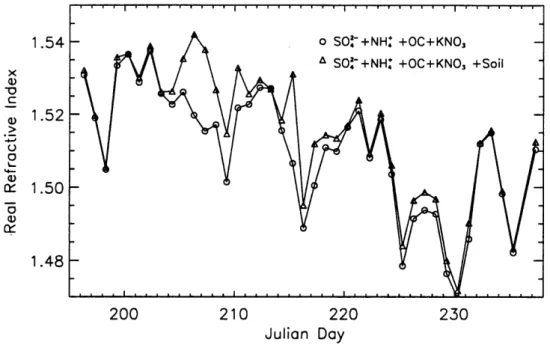
Calculations of daily dry real refractive indices were made using the partial molar refractive index method (Stelson, 1990). Chemical compounds (IMPROVE) included in the calculation were sulfate and ammonium (with associated hydrogen), organic carbon, and potassium nitrate. A small amount of water consistent with an ammonium bisulfate
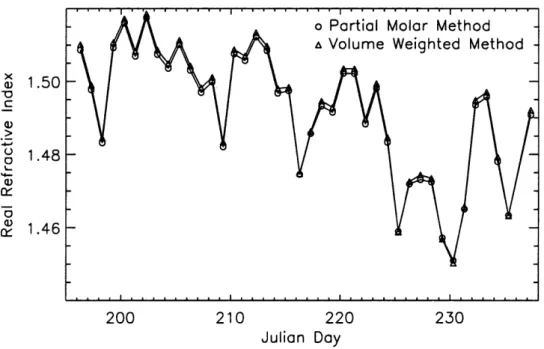
compound at 15% relative humidity was also included. Volume weighted refractive indices were computed for comparison, and the two methods were in good agreement. Complex refractive indices were calculated separately by including elemental carbon.
Wet refractive indices were determined using a newly-developed iterative method. Inputs included dry aerosol density, dry refractive index, aerosol mass and dry
accumulation mode volume concentration (derived from the ASASP-X). Wet refractive indices were used to invert high relative humidity AS ASP-X size distributions. Water mass was determined with the iterative method and compared to thennodynamically
predicted water mass assuming only ammonium and sulfate were hygroscopic (EQUILffi, Pilinis and Seinfeld, 1987). Comparisons of water mass ratios showed scatter around a 1:1 line, with 33 of the 61 total values corresponding to larger theoretical water mass ratios.
Results presented in this thesis include dry accumulation mode size parameters,
particle light scattering coefficients (bsp ), light scattering growth curves (blho )' and particle
hygroscopicity calculated from ratios of accumulation mode volume concentrations and volume median diameters. All of the results were calculated in two ways: from
distributions inverted with a rural aerosol model of refractive index, and using the daily
varying wet and dry refractive indices calculated in this thesis. Dry accumulation mode
parameters calculated from daily varying refractive indices increased slightly when compared to those calculated using the rural aerosol model. Comparisons of
hygroscopicity results suggested that this difference may cancel when ratioing parameters, resulting in similar aerosol growth values. Knowledge of the aerosol composition may therefore not be critical in making such observations.
Section 1.1. Experimental Background
Details of the experimental measurements taken during the SEA VS study were
provided in Ames and Kreidenweis (1996), however, a general overview will be provided
here to familiarize the reader with the motivation and methods for obtaining data, and to place the remainder of the thesis in context.
The field sight was located at Look Rock Tower (near Abrams Creek) at an
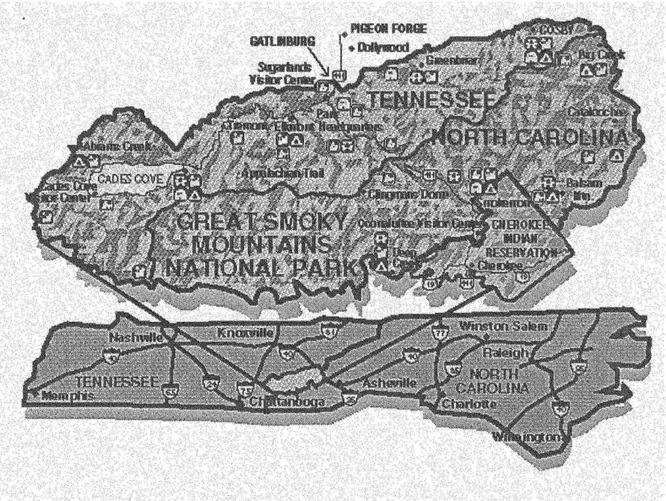
elevation of 793 meters, on the western edge of the Great Smoky Mountains National Park overlooking the Tennessee Valley and Cumberland Plateau. Figure 1.1 illustrates the
location of the sampling site and surrounding topography (Sherman et aI., 1997). The
National Park Service! Colorado State University study included the following
humidity (RH) dependent aerosol size distributions, RH dependent and ambient particle light scattering measurements, and local meteorological conditions (Ames and
Kreidenweis, 1996).
Relative humidity dependent measurements were performed daily using a RH controlled inlet, from which a radiance research nephelometer and an optical particle counter (ASASP-X) sampled. Total particle number concentration was measured with a Condensation Nuclei Counter (CNC) both night and day. Ambient light scattering was measured with a bank of nephelometers. All experimental details of the measuring system and protocol can be found in Ames and Kreidenweis (1996) and Day et al . (1996).
Figure 1.1 Great Smoky Mountains National Park and surrounding area (Sherman et ai.
1997).
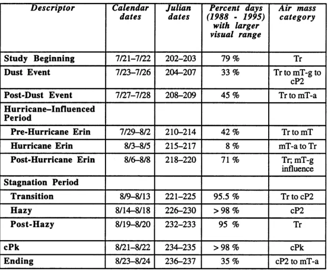
Unique meteorological periods occurring during SEA VS were characterized by Sherman et al. (1997). Table 1.1 summarizes specific meteorological events. These events
will be investigated in more detail later by evaluating differences in chemical composition, aerosol size parameters, and light scattering measurements during each period.
Table 1.1
Meteorological periods during SEA VS, as defined by Sherman et al. (1997).Classification of study periods was based on visibility conditions and synoptic scale air
mass source regions.
Descriptor
Calendar
Julian
Percent days
Air mass
dates
dates
(1988 - 1995)category
with larger
visual range
Study Beginning
7/21-7/22 202-203 79% TrDust Event
7/23-7/26 204-207 33% TrtomT-gtocP2
Post-Dust Event
7/27-7/28 208-209 45% Trto mT-aHurricane-Influenced
Period
Pre-Hurricane Erin
7/29-8/2 210-214 42% TrtomTHurricane Erin
8/3-8/5 215-217 8% mT-atoTrPost-Hurricane Erin
8/6-8/8 218-220 71 % Tr; mT-g influenceStagnation Period
Transition
8/9-8/13 221-225 95.5 % TrtocP2Hazy
8/14-8/18 226-230 >98% cP2Post-Hazy
8119-8/20 232-233 95 % TrcPk
8/21-8/22 234-235 >98% cPkEnding
8/23-8/24 236-237 35 % cP2 to mT-aCHAPTER 2: OPTICAL PARTICLE COUNTER
2.1. Theory
The optical particle counter used in this study was a Particle Measuring Systems (PMS) Active Scattering Aerosol Spectrometer Probe (ASASP-X). The measuring range
of the AS ASP-X (Dp
=
0.09 to 3.00 1J.D1) is divided into four overlapping size ranges, eachwith 15 size channels. Particles were sized with the following method. The light scattered by a particle passing through a He-Ne laser (A.=632.8 nm) was focused to a photodiode, which converted the intensity to a voltage. Depending on the magnitude of the voltage, the particle was classified into a particular size channel. This sizing depended upon the
manufacturer calibration which determined the relationship between voltage and size channel. The standardized calibration performed by PMS for the ASASP-X included polystyrene latex spheres (PSL) and glass beads. For each of the four ranges,
discriminator level voltages (DL V) were defmed for each of the 15 size chanriels. Each
range was normalized, so that the DL V varied from 0 to 10 volts. The voltage was
amplified by programmable amplifiers allowing it to be related to a specific diameter for all four ranges. The largest diameter range (range 0) corresponded to the smallest gain (smallest voltage amplification). For smaller size ranges, the voltage decreased and the range relative gain increased. A diameter-voltage relationship was thus established by the manufacturer. Figure 2.1.1 demonstrates the DL V for all ranges when normalized between 0 and 10 volts.
10.0 :- I I I I I I I ~ 1 0
§
~
~
0~
0 0 0 0 - 0 0 6. 0 0 0 6. 0 0 0 - 0 0 6. 0 0 0 6. 0 0 6. 0 en 0 6. 0....
0 0 1.0 ~ 0 6. 0 -> I-0 6. 0 l- I-6. I- 0 ~ 0 0 range 0 I- 0 range 1 0 6. range 2 I- 0 range 3 0 0.1 I I I I I I I 0 2 4 6 8 10 12 14 16 Bin NumberFigure 2.1.1. Discriminator level voltages (DLV) for the ASASP-X ranges.
Not taken into account during this calibration was the effect of refractive index on the light scattered from the particle. The smoothed manufacturer calibration was based on
PSL spheres (m =1.588-0i) ,and the resulting empirical relationship between voltage and
diameter assumed the instrument was insensitive to the optical properties of measured particles (PMS Manual, 1977). To correct the calibration for particles of other refractive index, Mie scattering theory was employed which assumed measured particles were spherical. Following the methods of Garvey and Pinnick (1983), Pinnick and Auvermann (1979), and Kim and Boatman (1990), the theoretical scattering response for the ASASP-X was calculated using the following equation:
{3
R =
~
J[IS\(6) + S\{1r-6)n+ [IS2(6) + S2(n -6)12jsin6d6 (2.1.1)where Sl x, m,9) and Six, m,9) are the Mie scattering functions corresponding to light with its electric vector polarized perpendicular and parallel to the scattering plane,
respectively. These functions depend on the index of refraction, m, the particle size
parameter, x=kr (k is the wavenumber and r is the particle radius), and the scattering angle
9. The integration is from a
=
350to
f3
=
1200, corresponding to the optics in the
ASASP-X. The BHMIE code provided in Bohren and Huffman (1983) was used to calculate Slx,
m,9) and Six, m,9). Theoretical response functions were then calculated for particles of different refractive index. Figure 2.1.2 provides examples of theoretical response
functions for different real refractive indices.
-
Q) 10-6-
CJ.-
~ s... 10-7 «S ~"
IIIS
10- B CJ--
Q) Ul 10- 9c
0 m=1.530 ~ Ul m=1.4BO Q) 10- 10 0::-
m=1.469 «S m=1.443 CJ.-
10- 11 ~ Q) m=1.420 s... 0 m=1.330 Q) 10- 12..c:
E-4 0.1 1.0 Particle Diameter (J..Lm)Figure 2.1.2. Theoretical response functions for the ASASP-X.
The experimental voltage was related to theoretical response by converting voltage
TR = DLV
NC· RG (2.1.2)
where NC is the nonnalization constant (V cm-2) and RG is the relative gain of a specific
range. Determination of NC and RG will be discussed in Section 2.3.
Refractive indices of atmospheric aerosols are generally significantly lower than that of PSL (Stelson, 1990). By not correcting the instrument calibration for true refractive index of a particle, measured sizes are underestimated, as reported by other researchers (Hering and McMurry, 1991; Kim and Boatman, 1990; Hand and Kreidenweis, 1996; Kim, 1995). This underestimation of aerosol size due to instrument calibration was the main motivation for developing a unique calibration for the ASASP-X in this thesis. The following sections detail the development of this calibration.
Section 2.2. Calibration
The calibration for the ASASP-X used in this thesis required determining the values
of the discriminator level voltages (DL V) for each diameter size channel, relative gains for
each range, and a normalization constant used to relate theoretical scattering cross-sections to experimental voltage values. The calibration developed here differs somewhat from that derived in Ames and Kreidenweis (1996) for the same instrument; sensitivity of results to
calibration procedures will be investigated by comparing results derived from two different
calibration methods (see Appendix A2).
Although the ASASP-X operating manual provided the values of discriminator level voltages, they were measured for this instrument after the field study concluded.
Details and descriptions of these measurements can be found in Ames and Kreidenweis
(1996), where the first experimental values determined were used in this work. These voltage values agree very well with those reported in the PMS manual.
To determine the relationship between theoretical particle scattering and
experimental voltages, measurements of PSL spheres were made because of their known monodisperse size and refractive index. Six sizes of PSL spheres from Interfacial Dynamic Corporation were used to calibrate the ASASP-X: 0.19, 0.25, 0.30, 0.41, 0.47, and 0.87
J..l.Ill diameter. Calibrations were performed both in the field and in the Atmospheric Simulation Laboratory at CSU after the conclusion of the study. PSL spheres were atomized and sampled with the ASASP-X both from the atomizer and after passing through a differential mobility analyzer (DMA) set to the corresponding voltage/size. The AS ASP-X channel corresponding to the maximum counts for a given size during these
measurements was the same for both sampling methods. More detailed discussion of this experiment can be found in Ames and Kreidenweis (1996). These measurements were used in this thesis to determine the relative gain and normalization constant for the
ASASP-X.
The measured DL V for each range were used to determine gain amplification. The channel voltage corresponding to the same diameter (assigned by PMS) in two consecutive ranges were ratioed to determine the gain between two ranges. For example, range 1, channels 10 and 14 overlap with range 0, channels 1 and 2. The lower limit channel voltage of range 1, channel 10 (0.957 V) was ratioed to range 1, channel 10 (5.356 V) to obtain a gain of 5.5967 between ranges 0 and 1. An average of all the overlapping
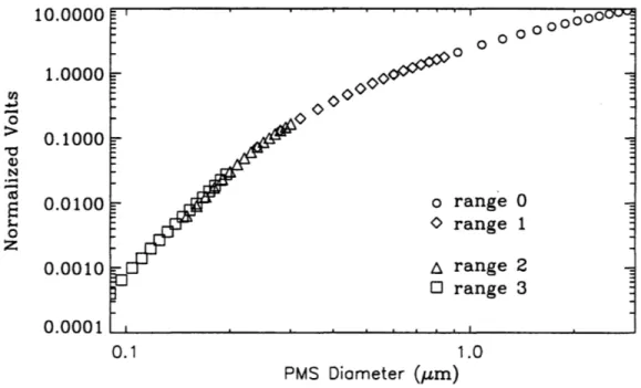
channels between these two ranges resulted in a gain of 5.62. This procedure was repeated for the other consecutive ranges to obtain average gain values between the other ranges. Figure 2.2.1 shows discriminator level voltages for all ranges normalized by their respective relative gains, resulting in a smooth, continuous calibration curve.
Because the PMS diameter assigned to a particular bin may not be accurate, the measurements of PSL spheres with diameters existing in the overlapping region of two size ranges were used to determine gain amplification as a check on the values used to obtain Figure 2.2.1. For each measurement, the channel corresponding to maximum counts was
recorded for the respective range. The upper and lower limit discriminator level voltages corresponding to the maximum count channel were averaged to obtain one voltage value
per channel, referred to as the maximum channel voltage (VM ) . For two overlapping
ranges, V M was ratioed to obtain the gain value between the two ranges. The same
procedure was performed for relevant PSL sizes in other ranges. Gains between ranges 0-1, 1-2, and 2-3 were obtained and then normalized by the gain for range O. These values
were typically within
±
20% of those derived from the first method described, using PMSdefined diameter bins (Figure 2.2.1).
rn ..,J
o
>
-0 Cl) N .-... 10.0000 1.0000 0.1000E
0.0100 s... o Z 0.0010 0 0 ~ 0 o 0000 0 0 0 0 rangea
range 1 range 2 range 3 0.0001~ __________ ~ __ ~ __ ~~~~~~~ ______ ~ __ ~ 0.1 1.0 PMS Diameter (J.Lm)Figure 2.2.1. Discriminator level voltages normalized by relative gain for the ASASP-X, derived using overlapping size channels.
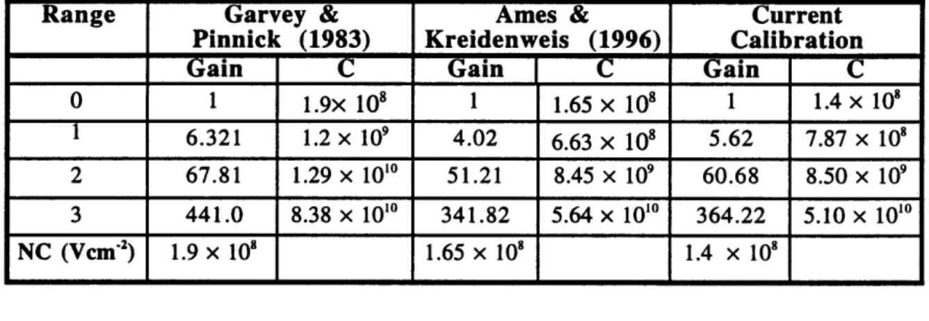
The relative gains (relative to range 0) used to create Figure 2.2.1 are reported in Table 2.2.1. Also reported in Table 2.2.1 are gain values from other investigators for comparison. Notice that the voltages in Figure 2.2.1 now fall between 0.0001 and 10 V in comparison to Figure 2.1.1 due to the normalization by relative gain.
To determine the nonnalization constant (V cm-2) which relates voltage to
theoretical response, Mie scattering response was calculated for m=1.588 (PSL) at each of
the PSL diameters used in the calibration. The maximum channel voltage (V M ) in which
that particle appeared was divided by the calculated scattering response value (cm2). For
the various PSL sizes included in the calibration, an average NC of 1.4x 10⁸ V cm-2 was
obtained. The product of NC and RG (denoted C ) provides a comparison of the
constant used to nonnalize each range. These values are also found in Table 2.2.1, along with values used in previous studies.
Table 2.2.1 Relative gains for each range, with the corresponding nonnalization constant.
Range Garvey & Ames & Current
Pinnick (1983) Kreidenweis (1996) Calibration
Gain C Gain C Gain C
0 1 1.9x 10⁸ 1 1.65 X 10⁸ 1 1.4 X 10⁸ 1 6.321 1.2 x 10⁹ 4.02 6.63 x 10⁸ 5.62 7.87 x 10⁸ 2 67.81 1.29 x 10¹⁰ 51.21 8.45 x 10⁹ 60.68 8.50 x 10⁹ 3 441.0 8.38 x 10¹⁰ 341.82 5.64 x 10¹⁰ 364.22 5.10 x 10¹⁰ NC (Vcmo1) 1.9 x 10⁸ 1.65 X 10⁸ 1.4 X 10⁸
The constants derived in this thesis tend to be lower, or fall between the constants
presented by other investigators. The effects of this smaller nonnalization constant will be investigated in Appendix A2. Determination of channel limit diameter is discussed in the following section.
Section 2.3. Determination of Channel Diameters
To determine the diameter-channel relationship, the nonnalization constant, NC ,
normalized DL V in each range. Two diameter-channel relationships will be derived in this section, those for m=1.588 (PSL) and m=1.530, corresponding to dry ammonium
sulfate. Figure 2.3.1 shows the Mie theoretical response for m=1.588 (PSL). Also plotted
on Figure 2.3.1 is the diameter-voltage relationship for PMS defined diameters with DL V converted to scattering response using NC =1.4x10⁸ V cm-2• For smaller particles, a
shift in diameter values was required because the PMS defmed channel-diameters do not fall directly on the Mie theoretical scattering response. The newly-defmed diameters required to "match up" channel limit scattering response and Mie theoretical response were determined by an interpolation method. Figure 2.3.1 demonstrates the differences between these diameters. 10-7
-
Q) Cj....
~ 10-8 s.. «S 0.. ~e
CJ 10-9 ... Q) rn I::: 0 0.. 10- 10 rn Q) 0::-
«S .~ 10- 11 ~ Q) s.. 0 Q) .a E-o 10- 12 0.1Derived Diameters for m= 1 .588
Diameter (JLm) f). o 1.0 Derived PMS
Figure 2.3.1 Derived and PMS diameters for PSL (m = 1.588).
Due to the overlapping nature of the ASASP-X size ranges, a scheme for dealing with measured counts in the overlapping size channels was required. In developing this
scheme, the 60 original size channels were reduced to 34. As discussed in Ames and Kreidenweis (1996), the discriminator level voltages in ranges 2 and 3 had more
experimental measurement uncertainty than in the larger size ranges. In these lowest two ranges, two to three size channels were grouped together to account for the noise in voltage measurements. In the lowest size range (range 3), the fIrst and second channels were discarded completely. In other ranges, 2 to 3 consecutive size channels were grouped together, leading to fewer overall channels. This method was similar to that in Ames and Kreidenweis (1996). The overlapping scheme used in this work was simplifIed by the continuous voltage calibration curve derived in the previous section. The size channels in overlapping regions lie directly on top of one another (see Figure 2.2.1), allowing for some channels to be discarded. The particles with diameters corresponding to the upper end of a size range were sized with more precision than at the lower end (PMS Manual, 1977). Whenever possible, the lower channels of an overlapping range were therefore discarded while the upper channels of the smaller range were retained. This method for dealing with overlapping size ranges resulted in no averaging of counts between channels.
Previous researchers have investigated the effects of the multi valued region of the Mie theoretical response on size distributions (Hering and McMurry, 1990; Kim, 1995, Richards et aI., 1985; Pueschel et al., 1990). For PSL, this region occurs around Dp
=
0.4- 0.6 J.lm (see Figure 2.3.1). For a particular theoretical response, a unique diameter cannot be determined in this range. In deriving size channels in this region, two methods were investigated: smoothing through the region, and lumping the entire diameter range into one channel. Although the lumped diameter method seemed more appropriate,
applying it in the calibration resulted in unusual peaks and dips in the number distributions which were suspect. Similar results were obtained by Pueschel et. al (1990) for a similar calibration. A smoothed set of diameters falling parallel to the original PMS calibration was therefore applied in the multi valued region. The resonances in the Mie theoretical response curve corresponding to Dp > 1.0 J.lm made it difficult to assign diameters to size channels
in this region. PMS defined diameters were therefore chosen in the largest size range (range 0).
The final 34 size channels correspond to a specific set of scattering response values
(cm2). These scattering values remain constant; determining the corresponding particle
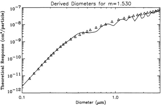
diameters for a different refractive index requires shifting the diameters to the respective Mie theoretical response curve (Hand and Kreidenweis, 1996). Figures 2.3.1 and 2.3.2 show the resulting channels for m=I.588 and m=I.530. Table 2.3.1 reports the lower
channel limit scattering response and diameter derived for m = 1.588 and m = 1.530.
10-7 Derived Diameters for m= 1.530
-
Q) '0 ... ~ 10-8 s.. «S 0..:;--.
e
0 10- 9-
Q) en d 0 0.. 10- 10 en Q) 0:: ta 0 :;:; 10- 11 Q) s.. 0 Q) ..c:: E-< 10- 12 0.1 1.0 Diameter ().Lm)Figure 2.3.2. Derived diameters for m = 1.530, with the corresponding Mie theoretical response.
Two consistency checks were made on this diameter set. The first check was performed using PSL calibration measurements. The PSL data.were inverted using the
derived smoothed diameter set for m = 1.588. A lognormal fitting program (DISTFIT,
Table 2.3.1. Lower limit channel response and diameter for m = 1.588 and m=I.530. Bin Scattering m= 1.588 m=1.530 Cross-Section (cm-2 ) Dp (Ilm) Dp(llm) 1 7.0856x10⁻¹² 0.116 0.120 2 1.4128x10⁻¹¹ 0.130 0.134 3 2.5671x10⁻¹¹ 0.143 0.149 4 4.3478x10⁻¹¹ 0.157 0.162 5 6.9424x10⁻¹¹ 0.170 0.176 6 1.0682x 1 0-10 0.183 0.190 7 1.6430x 1 0-10 0.197 0.204 8 2.1621x10⁻¹o 0.208 0.216 9 3.4936x10⁻¹O 0.228 0.236 10 5.1980x10⁻¹O 0.248 0.257 11 7.1496x10⁻¹O 0.266 0.275 12 9.3706x10⁻¹o 0.283 0.293 13 1.4306x10⁻⁹ 0.320 0.331 14 1. 9887x 1 0-9 0.360 0.370 15 2.6176x10⁻⁹ 0.400 0.414 16 3.3149x10⁻⁹ 0.440 0.452 17 4.1036x10⁻⁹ 0.480 0.497 18 4.9609x10⁻⁹ 0.520 0.538 19 6.8025x10⁻⁹ 0.600 0.621 20 8.7250x10⁻⁹ 0.680 0.704 21 1.0663x10⁻⁸ 0.760 0.787 22 1.5136x10⁻⁸ 0.920 0.920 23 1. 9700x 1 0-8 1.08 1.08 24 2.4286x 1 0-8 1.24 1.24 25 2.8936x10⁻⁸ 1.40 1.40 26 3.3493x10⁻⁸ 1.56 1.56 27 3.7757x10⁻⁸ 1.72 1.72 28 4.2193x10⁻⁸ 1.88 1.88 29 4.6643x10⁻⁸ 2.04 2.04 30 5.1086x10⁻⁸ 2.20 2.20 31 5.5379x10⁻⁸ 2.36 2.36 32 5.9629x10⁻⁸ 2.52 2.52 33 6.3707x10⁻⁸ 2.68 2.68 34 6.7567x10⁻⁸ 2.84 2.84 7.1471x10⁻⁸ 3.00 3.00
median diameter was compared to the indicated PSL diameter, to determine if the particles were sized correctly. Of particular interest was the comparison of PSL particle sizes in the
multivalue region. For the instrument calibrations performed during SEA VS with 0.41
J.1m PSL particles, an average number median diameter of 0.413
±
0.007 J.1m wasdetermined. Figure 2.3.3 provides an example of a PSL (0.41 J.1m) number distribution and
corresponding lognormal curve fit.
Aerosol Number Distribution
4000 m = 1.58800 PSL
EN
227.802 -n I 3000E
Dp1n 0.419000 (,) - . " 0.. 1.05500 0 u=gn
2000 g -'ljX
2 = ... 0.122000z
'lj 1000 JD 195.661 0 0.1 1.0 Dp (J.Lm)Figure 2.3.3. PSL (D p
=
0.41 J.1m) number distribution and lognormal fit.This check was also used to investigate the effects of a lumped versus smoothed diameter set through the multivalue region. When using a lumped diameter channel in the multivalue region, fit number median diameters were different from the known PSL diameters due to the width of the channel where maximum counts occurred. The distribution was also fit with a larger geometric standard deviation. For the smoothed
diameter set, the median diameters always agreed very well with PSL indicated diameters, and reasonable geometric standard deviations were determined. It should be noted that for the 0.21 J.1m PSL, the lognormal curve fits consistently resulted in a median diameter of 0.25 J.1m, while the 0.19 J.1m PSL particles agreed well with the lognormal number median diameter. Because both of these PSL particles were sized in range 2 (two to three channels apart), it was concluded that there was some discrepancy with the 0.21 J.1m PSL spheres.
The second check performed on the diameter set involved the overlapping size ranges. As noted in Figure 2.2.1, when normalized by the appropriate relative gain, the discriminator level voltages resulted in a continuous calibration curve. For the overlapping size channels, the number of counts in each channel should be the same. For example, in range 3, channels 10-13 overlap with range 2, channell. The sum of the counts in channels 10-13 (range 3) and the counts in channell (range 2) should be the same if the relative gains were appropriate. For all ranges, these comparisons were very close, with an average percent difference in counts of 0.01 %. Based on these checks, the diameters derived in this thesis were assumed to be an appropriate calibration choice and were used to invert ASASP-X data.
Section 2.4. Diameter Scaling Method
The re-calibration of channel diameters based on refractive index in Section 2.3 was a time-consuming and tedious process. A method by which a set of diameters could be scaled based on refractive index was needed and will be developed in this section. The motivation for developing a scaling method will become apparent in Chapter 4 when daily varying refractive indices of dry aerosol measured during SEA VS will be calculated. Speedy derivation of diameters for arbitrary refractive index will be essential for ASASP-X data inversion.
As seen in Figure 2.1.2, Mie theoretical response curves (TR ) for a variety of real refractive indices have basically the same shape: linear from Dp 0.1 - 0.4 J.1m, a resonance (multivalue) region from Dp= 0.4 - 0.6 J.1m, and resonances when Dp > 1 J.1m. Being able to relate Mie scattering curves to one another was essential in this scaling process. The theoretical response for a 0.1
J.1II1
diameter particle for real refractive indices ranging fromm = 1.33 to 1.530 were calculated from equation (2.1.1). The ratio of the theoretical response value at Dp
=
0.1 J.1m for a given refractive index (TRj ) and for that of m=
1.530(TRJ.53oJ was determined, as in equation (2.4.1):
f. - TR1.530
TR.i - TR.
1
(2.4.1)
Scattering values for particle diameters ranging from 0.1 - 3.0 J.1m corresponding to a given refractive index were multiplied by
iTR ,
resulting in a "collapse" of the Mie curve to the m= 1.530 position (see Figure 2.4.1).
-
Q)-
0 .-~ s.. a:s P.. "'-... N6
0---
Q) Ul d 0 P.. Ul Q) ~-
a:s 0 :;; Q) s.. 0 Q) ..c:: E-t 10- 6 10- 7 10- B 10- 9 10- 10 10- 11 10- 12 0.1 1.0 Particle Diameter (fLm)Figure 2.4.1 "Collapsed" Mie curves around m =1.530.
m=1.530 m=1.4BO m=1.469 m=1.443 m=1.420 m=1.330
The scaling factor for the theoretical response
if
TR) needed to be translated to adiameter scaling factor'!D' By performing a linear regression in the 0.1 - 0.4 J.UI1 diameter
range on the original and "collapsed" Mie curves for a given refractive index, two linear
equations of the fonn TR = aD p
+
b were determined, where a was the slope, and b wasthe intercept. These two equations were used to determine a diameter scaling factor in the following way.
Two values of scattering response were chosen (lxlO-lo and Ix 10-9 cm2/particle).
These were substituted into both the original and "collapsed" linear equations, from which
the values of Dp were determined. A ratio of the original and scaled diameters resulted in a
diameter scaling factor'!D' analogous to the theoretical response scaling factor,! TR' A fit of
!D versus real refractive index (Figure 2.4.2) resulted in a polynomial, equation (2.4.2),
with a correlation coefficient of R2 = 0.9999,
fo
=
1.759m2 - 5.9873m + 6.0436 (2.4.2)where m is refractive index. By using this equation, an original set of diameters
(m=1.530) were scaled to a new refractive index by calculating!D' and multiplying all
diameters in the original set bY!De
Although this scaling was determined from a specific set of seven refractive indices, it was also successfully applied for other refractive indices not used in the development of the equation (see Figure 2.4.3). The advantages of this scaling included a quick
determination of new diameters to expedite data inversion, and scaling of diameters in the
region D p
>
1 Jlm where resonances in scattering response make it difficult to detennine aunique diameter. The disadvantage was that for a refractive index approaching that of water, the Mie curves flatten and the scaling becomes less appropriate (see Figure 2.4.3). The lowest refractive indices in this study for which this scaling procedure will be applied
rural aerosol model for refractive index as a function of relative humidity. In Chapter 6, it
will be applied to derived daily refractive indices.
Diameter Scaling Factors
1.20
-
'tJ -"'-" I... 1.15 0 ... u 0-
0'1 c 1.10 0 u en I... Q) ... Q) 1.05 E .2 "'0 1.35 1.40 1.45 1.50 refractive indexm-l.330 smoothed bins 10-7~----~--~~--~-T~~----~--~ 0.1 1.0 Dp (,aD) m= 1.42 smoothed bins 10-7---~--~~~~-T~~----~--~ 10-12~ ____ ~ __ ~~~~~~~ ____ ~~~ 0.1 1.0 Dp (,aD) m=1.501 smoothed bins 10-7~----~--~~~~~~~----~~~ 10-12L.-____ ~ __ ~~ ... ~~~~ ____ ~ __ ~ 0.1 1.0 Dp Uun) m-1.380 smoothed bins 10-7~----~--~~--~~~~----~~~ 0.1 1.0 Dp Uun) m= 1.469 smoolhedbins 10-7~----~--~~~~~~~----~~~ Dp (,aD) m=-1.520 smoothed bins 10-7~----~--~~--~-T~~----~--~ Dp Uun)
CHAPTER 3. DATA INVERSION AND RESULTS USING A RURAL AEROSOL MODEL REFRACTIVE INDEX
The initial ASASP-X data inversion was performed by employing a rural aerosol model of refractive index based on relative humidity (Shettle and Fenn, 1979). The values of refractive index used in Ames and Kreidenweis (1996) were applied in this section for data inversion and can be found in Table 3.1.1. No absorbing characteristics of the aerosol were considered, therefore the imaginary part of the complex refractive index was ignored.
Table 3.1.1. Rural aerosol model of refractive index
Relative Real refractive Interpolated Relative humidity
Humidity index, m, for values of of applied
(%)
rural aerosol refractive refractive indexmodel index, m
(%)
(Shettle and Fenn.1979)
Dry 1.530-0.00660 i 1.530 40>RH 50 1.520-0.00626 i 1.520 40<RH<60 70 1.501-0.00560 i 1.501 60<RH<73 75 1.469 73 <RH <77 80 1.443-0.00370 i 1.443 77 <RH <83 85 1.420 83<RH
The calibration used for data inversion was described in the previous sections, and diameter size channels as a function of refractive index were determined using the scaling procedure described in Section 2.4. The results presented in this section include dry accumulation mode size distribution parameters, hygroscopicity, and particle light scattering. The present results differ from those in Ames and Kreidenweis (1996) in two respects: the new calibration and refractive index scaling of instrument response, and the fitting of a lognormal size distribution function to the data. In Appendix A, sensitivity studies are presented to demonstrate the effects of these different assumptions on the derived results.
Section 3.1. Lognormal Size Distribution Function.
Atmospheric aerosol size distributions are often conveniently described as a lognormal size distribution function of the form (Seinfeld, 1986):
n(lnDp ) (3.1.1)
where Dpg,n is the number median diameter, O'g is the geometric standard deviation, Dp
is the particle diameter, and N is the total number concentration. From these parameters,
other size distribution parameters can be derived. Total volume concentration was calculated from equation (3.1.2).
1C 3
V = '6NDpvm (3.1.2)
where Dpvm is the volume mean diameter and is given by equation (3.1.3).
Dpvm
=
-Dpg,n exp(1.5 ·In 2 O'g) (3.1.3)The volume median diameter, Dpgv' was calculated from equation (3.1.4).
(3.1.4)
To determine ASASP-X size distribution parameters, the DISTFIT lognormal fitting program (Whitby, 1991) was employed. Single mode lognormal functions were fit
Jlm) of the distribution. The reasons for fitting the lognormal size distribution function to the ASASP-X data were threefold. The first reason is demonstrated by a sample SEAVS ASASP-X aerosol volume distribution in Figure 3.1.1.
Aerosol Volume Distribution
12
-
10 fte
0"-
8 ne
::t DpiY 0.240000 EV 3.98000 ' - ' 0.. 6 JD 205.748 0 0.0 RH 0-
4 "tj "-> "tj 2 0 0.1 1.0 Op ().Lm)Figure 3.1.1. Sample SEA VS aerosol volume distribution.
An obvious decrease in the distribution around Dp= 0.4 Jlm in Figure 3.1.1 is often
noticeable in distributions measured with optical particle counters and is most likely an artifact of the flat region of the Mie response curve in that size range (Hering and
McMurry, 1991, Richards, et al., 1985). This large decrease in the size distribution was
smoothed by the lognormal curve (see Figure 3.1.1).
The second reason for fitting the data was that the lognormal function was
capable of capturing particle sizes smaller than the measuring range of the ASASP-X (Dp
<
0.1 Jlm). By including these sizes, a more realistic approximation of the accumulationdiameter, Dpg,n, was computed. This parameter was unobtainable using the method in
Ames and Kreidenweis (1996) because the smaller size range of the number distribution was not captured. The number distribution parameters were required for light scattering calculations, as discussed in Section 3.3.
6000 __ 5000 n I
8
~ 4000 Poto
gn
3000:a
"
~ 2000 1000Aerosol Number Distribution
/ / / / / I EN 2677.27 DplD 0.152000
a.=
1.73300 RH=
79 % JD 223.545 o~__
~__
~~/~~~~__
~__
~~~~~____
~~~~ 0.01 0.10 1.00 Dp (J.Lm)Figure 3.1.2. Sample SEA VS number distribution. The dashed line corresponds to the lognormal curve and demonstrates the extrapolated part of the distribution.
Finally, the fitting automatically determined the accumulation mode for each distribution whereas the accumulation mode cut-off diameter had to be chosen arbitrarily in Ames and Kreidenweis (1996). Comparisons of derived quantities assuming no size distribution function were compared to results obtained using the lognormal fit (see Appendix A), and showed good agreement between the two methods.
~ Dry Total Number Concentration (cm-3 )
'5
2500~----~----~,~---~---.~---~--~--~---~----~ - 2000 , •~
1500 • • • • "i,· •
8J
,. .,,, , ••
Ie •• • , . ~ 1 0 0 0 . .I . ' . ..
. •.
iii 500 ' . , • O • • • ~ ~----~---~---~----~---~--~ E- 200 210 220 230 Julian DayDry Total Volume Concentration (JLm3
/cm3 ) ~ 25~----~--~---~---~~--~--~--~--~ o 20 • ;:--.. 8 15
J
..; 10&
•
, .
f·
§
5··
,It,.".,.,.;,_.
..,.,'
o
O~ ____ ~ ____________ ~ ______ ~~ ____ ~ ________________ ~ > 200 210 220 230 Julian Day Dry Dpg,v (JLm) 0.34 ;... •-8'
0.32 j , . • ~ :to 0.30 ~ • • : , , • • • - .. - 0.28 - • . . . .-:0
0.26 ~ • , • • • • , •-&
0.24 ~ • •• & .. • : , , .-8:~~ 1:..~
_ _ --a... _ _ _"--.;::iI:t...--_---....;\_, __
, ___
... _____
--,-_...::I-200 210 220 230 Julian Day Dry Dpg,n (JLm) 0.24 :- • -:
8'
0.22 ~ • , • , • , :to 0.20 ~ • • - 0.18 :- • , •• : , . . . • • •1.
!
-~ 0.16 ;;.. .. , , • • • Q. 0.14 ~S \ • •• '
•
Q 8:l~~:-_____________________ •
__________________________
~__
~-: 1.6 1.5 ~ • t ' . b 1.4 ,... 1.3 '-200 200 210 220 230 Julian DayDry Geometric Standard Deviation
«(]
11.)•
•
~:
..
'
,"
..
.
....
-,
..
•
•
210 Julian Day•
·,1
~,
,.
:
.
,."t··
-220 230Timelines of dry accumulation mode size parameters calculated for dry
(RH<15%) aerosol are presented in Figure 3.1.3 for JD 195-232. The trends in the size
parameters tended to follow the meteorological trends occurring in the site region, as defined in Shennan et al. (1997) (see Table 1.1 in Chapter 1). Most noticeably, accumulation mode total number and volume concentrations increased during the
extreme haze period at the end of the study. The geometric standard deviation, Gg,
remained very stable during this period. Study averages for dry accumulation mode
aerosollognonnal size parameters assuming a real dry refractive index of m = 1.530 are
reported in Table 3.1.2.
Table 3.1.2. Dry accumulation mode lognonnal size parameters for dry real refractive
index of m
=
1.530.Size Study Standard Study Study
Parameter Average Deviation Maximum Minimum
N (cm-3 ) 1200 ±5oo 2384 145 V {Jlm3cm-3 ) 7 ±4 21.77 0.98 Dpg,n (J.1m) 0.17 ±0.03 0.232 0.116 DDIl.v (J.1m) 0.26 ±0.03 0.331 0.206 0'11 1.45 ±0.06 1.664 1.353
Section 3.2. Particle Hygroscopicity
The major objective of the CSU SEA VS experiment was the determination of aerosol hygroscopicity. A solid aerosol particle will remain in crystalline fonn until a thennodynamically preferred relative humidity satisfying equation 3.2.1 is reached (tenned the relative humidity of deliquescence, RHD)
where aw . .SIU is the water activity of the saturated solution (Tang, 1996). Equation (3.2.1)
ignores the Kelvin effect, which is generally unimportant for Dp> 0.1
JlD1
forthehumidities examined in this study. At the RHO, the particle will spontaneously begin to take up water (deliquesce) and grow. As relative humidity is increased, equilibrium between the aerosol particle and the surrounding water vapor is maintained and the particle continues to grow with the addition of water according to a growth curve
corresponding to its particular composition. For the same solution drop which is dried, a hysteresis effect is demonstrated when the particle "descends" on a different branch (efflorescence) than that of the deliquescence curve. The particle will release water and return to crystalline form at a relative humidity lower than the RHO. Figure 3.2.1 shows
the hysteresis effect for ammonium sulfate (Nemesure et al., 1995). Different pure salts
demonstrate different growth characteristics depending on their corresponding RHO and solution thermodynamics, as demonstrated in Figure 3.2.1 for the ammonium sulfate system. 2.0
r2
1.8~
1.8 1.4-1.2...
----
...
I' (NH. )2 SO.I:
NH .. HSO.. i, ow ow i'Ra
SO. ,. I i'-.-
---_
...
,.
,
FO ,,.
,
,.
,.
/0 I ~.,. " I .~,
~-,,'
_ - - - I 1.0~ __ -_-__ ~ ______ ~· ______ ~ ______ ~ ______ ~o
20 40 80 80 100 RelaUve lIumidlty. XFigure 3.2.1 Hygroscopic growth for the ammonium sulfate system (Nemesure et al.,
1995)
Hygroscopicity of the aerosol measured during SEA VS was calculated using ratios of lognormal size parameters. The pairs of wet and dry distributions used to calculate these ratios were the same as those in Ames and Kreidenweis (1996). Two
wet to dry accumulation mode total volume concentration (DyID y.o)' Equations 3.2.2 and 3.2.3 were used to calculate growth curves from wet-to-dry diameter and volume ratios, respectively: Dd Dpgv.wet - - = D d,o D pgv. dry (3.2.2) (3.2.3)
Figures 3.2.2(a) and 3.2.2(b) show the resulting growth curves for both methods, with fourth-order polynomial fits to the data. Values of DvIDv.o demonstrated more scatter
than diameter ratios but with larger growth at higher RH. Tang et ale (1978) showed that
pure sulfate particles had growth factors ranging from 1.5 to 1.8 at 80 % RH, depending
on the particle acidity. Svenningsson et ai. (1992) observed two hygroscopic modes
when measuring hygroscopic growth. At 85 % RH, the more-hygroscopic mode mean
growth factor was 1.44
±
0.14 while the less-hygroscopic mode mean growth was 1.1±
0.07, with no significant size dependence. Svenningsson et ai. (1992) concluded that both
the hygroscopic modes included insoluble material because the measured growth was much less than that of pure salt. Two hygroscopic modes were previously observed by
other investigators (McMurry and Liu, 1978; McMurry and Stolzenburg, 1989; Covert et
aI., 1991). It was suggested by Svenningsson et ale (1992) that the less-hygroscopic mode probably contained soot and organics, while the more-hygroscopic mode most likely consisted of more soluble material such as the major ions, along with some insoluble material. From the fourth-order polynomials plotted in Figures 3.2.2 (a,b), the hygroscopic growth at 85% for the rural aerosol model varied between 1.24 and 1.28 depending on the method of calculation. These results fell between the values obtained
by Svenningsson et ai. (1992), suggesting some insoluble material was present. A
shape; no abrupt change in DIDo occurred for any RH, suggesting the particles were measured on the efflorescence curve, or their composition was something that deliquesced at low RH. More discussion of this feature can be found in Section 4.4.
1.40 1.30
o
" a 1.20 1.10 1.00o
y= 1.983e-8x· - 2.41ge-6x3+
1 .082e-04x2 - 1. 1 5ge-3x+
1 .00 o o o o 0 00 a:J o 0 -g-~--~---o 20 40 60 80 Relative Humidity (%)Figure 3.2.2(a) Hygroscopic growth using diameter ratios.
1.40 1.30 o a " a 1.20 1.10 1.00
o
y= 2.304e-8x· - 3.046e-6x3+
1.554e-04x2 - 1.947e-3x+
1.00 o o o o 0 0 0 0 o o o 00 o 0 _J:J _ _ --~----~---o 0 o o 20 40 60 80 Relative Humidity (%)Figure 3.2.2(b) Hygroscopic growth using volume ratios.
Section 3.3. Particle Light Scattering (b ,,)
Light extinction is contributed to by several components, and the extinction coefficient can be described by equation 3.3.1 (in units of inverse length):
(3.3.1)
where bsp and bap correspond to scattering and absorption by particles, respectively, and
b sg and bag are scattering and absorption by gases. Absorption by particles is due mainly
to elemental carbon (soot). Scattering by air molecules is called Rayleigh scattering and
the major absorbing gas is nitrogen dioxide. Particle light scattering coefficients can be
calculated from equation 3.3.2, where the subscript denoting scattering (sp ) is replaced
by (ap ), if the absorption coefficient is desired.
b sp =
j
~Qsp
(x, A, m)D; ( dN JdlOgD po 4 dlogDp (3.3.2)
The Mie scattering efficiency, Qsp' is a function of size parameter (x=1dJ/A), scattered
wavelength of light,
A,
and particle refractive index, m. The calculation of scatteringcoefficient, bsp' also depends upon the aerosol number size distribution (dN/dlogDp) and
the geometric area of the particles (D/) (Hegg, et al., 1993).
For calculations performed using ASASP-X number distributions, the lognormal size function was convenient to use in a numerical integration of equation 3.3.2. The
lognormal number size distribution was divided into 100 size bins, evenly spaced in InDp '
ranging from 0.01 - 10 Jlm. The number concentration in each bin was calculated using
the difference of a cumulative distribution function, F(Dp)' calculated at bin diameters Dp•i
F(O .) = N + N erf(ln(Op'i/Dpg,n)]
p,l 2 2 .J2ln(1
g
(3.3.3)
where N, Dpg ,n ' and (1g were defined as lognormal parameters. The particle bin
boundary diameter is given by D p.i ' and erf is the error function. The bin number
concentration, Nil determined from equation (3.3.4), was summed over all bins and
compared with the total lognormal number concentration, N, to assure consistency.
(3.3.4)
The midpoint bin diameter, Dpm,i' of each bin was calculated with equation (3.3.5), and
converted into the size parameter with
A
= 0.530 Jlm, chosen to represent the midpoint ofthe visible spectrum.
(3.3.5)
Scattering efficiency, Qslx, m, A) ,was calculated using Mie theory (Bohren and
Huffman, 1983), assuming spherical, internally mixed homogeneous particles. For each
bin, the scattering efficiency, Qsp , and scattering coefficient were calculated using
equation (3.3.6) at the midpoint diameter. The refractive index applied in this calibration
corresponded to those in the rural aerosol model. For dry (RH < 15%) distributions, the
refractive index was always taken to be m = 1.530.
1C 2
The total scattering coefficient, hsp , was then calculated by equation (3.3.7).
(3.3.7)
Figure 3.3.1 shows timelines of hsp (km-I) for dry (RH<15%, m=1.530)
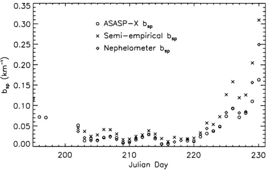
accumulation mode aerosol with a study average of 0.044 km-I. Nephelometer
measurements at SEA VS showed good agreement, except for the last two days when the nephelometer was unreliable (Day et aI., 1996). The scattering coefficients calculated from a semi-empirical fit based on work by Malm et aI. (1994a), given by equation (3.3.8), are also plotted.
bsp == effdrum [sulfate]J(RH) + 0.003[Inorg]J(RH) + O.OO4[OC] + 0.001 [soil] (3.3.8)
(Equation (3.3.8) from Derek Day, personal communication). The closed brackets in equation (3.3.8) denotes species concentration in J.lg m-3• The coefficients thus represent
species mass scattering efficiencies. The term efhrum is the mass scattering efficiency of sulfate computed from daily DRUM sampler measurements made during SEA VS. The growth term, (f(RH)), which appears in the first and second terms, represents the change in mass scattering efficiency with relative humidity for hygroscopic particles (Malm et
ai.,
1994b). The dry scattering efficiency for organic carbon was taken as 0.004 km-IJ.lgm-3 and for soil as 0.00 1 km-I J.lg m-3• The soil constituents for this calculation were
assumed to be silicon, aluminum, and iron. Inorganic aerosol, [inorg], included N03-, Na+, and CI-, and a dry scattering efficiency of 0.003 km-IJ.lg m-3 was assumed for these.
The trends were consistent with meteorological periods, e.g., bsp increased during the hazy event, when decreased visibility was expected. Although trends agreed for the two methods of computing hsp , ASASP-X data were significantly lower than those using
the semi-empirical relationship, as shown in Figure 3.3.1. From equation (3.3.2), the
components which affect the calculations of hsp were the scattering efficiency, Qsp' the
particle area, D p 2, and the number distribution. If the refractive index used in the
calculation was smaller, the scattering would decrease, but the inverted size distributions
would lead to larger size parameters. Tang (1996) and Hegg et ale (1993) found that in
calculations of light scattering coefficients, the chemical effect (species composition) is
outweighed by the size effect. In Chapter 6, the effects of lower refractive index and
larger particle area will be investigated.
0.35 0.30 0.25 g. 0.15 .0 0.10 0.05 200 o ASASP-X bsp x Semi-empirical bsp o Nephelometer bsp 210 Julian Day 220 x x x oOo@ xo 0 x o 230
Figure 3.3.1 Timeline of dry hsp (kIn-I) for rural aerosol model (RH < 15%, m = 1.530)
plotted with nephelometer measurements and semi-empirical estimates.
Section 3.4. Particle Light Scattering Growth Curve (bib 0 )
As mentioned in the previous section, the effects of relative humidity on
scattering efficiencies for hygroscopic particles will modify the particle light scattering
coefficient, h sp• As particles take up water, light scattering characteristics change
through decreased refractive index, and increased size (area). Ames and Kreidenweis (1996) demonstrated the effects of increased relative humidity on scattering coefficients