Learning Stochastic Nonlinear Dynamical Systems Using Non-stationary Linear Predictors

Using Non-stationary Linear Predictors

MOHAMED RASHEED-HILMY ABDALMOATY

Licentiate Thesis

Stockholm, Sweden

TRITA-EE 2017:172 ISSN 1653-5146

ISBN 978-91-7729-624-9

School of Electrical Engineering Department of Automatic Control SE-100 44 Stockholm SWEDEN Akademisk avhandling som med tillst˚and av Kungliga Tekniska h¨ogskolan framl¨agges till offentlig granskning f¨or avl¨aggande av teknologie licenciatexamen i elektro- och systemteknik onsdag den 20 december 2017 klockan 10.00 i H¨orsal Q2 (rumsnr B:218), Osquldas v¨ag 10, Q-huset, v˚aningsplan 2, KTH Campus, Stockholm. © Mohamed Rasheed-Hilmy Abdalmoaty, November 2017.

All rights reserved.

Nonlinear stochastic parametric models are widely used in various fields whenever linear models are not adequate. However, the problem of parameter identification is very challenging for such models; the likelihood function – which is the central object in statistical inference – is, in general, analytically intractable. This renders favored point estimation methods, such as the maximum likelihood method and the prediction error methods, analytically intractable. In recent years, several methods have been developed to approximate the maximum likelihood estimator and the optimal mean-square error predictor using Monte Carlo approximation methods. However, the available algorithms can be computationally expensive; their application is so far limited to cases where fundamental difficulties, such as sample degeneracy and impoverishment problems, can be avoided.

The contributions of this thesis can be divided into two main parts. In the first part, several approximate solutions to the maximum likelihood problem are explored. Both analytical and numerical approaches, based on the expectation-maximization algorithm and the quasi-Newton algorithm, are considered. The performance of the developed algorithms is demonstrated on several numerical examples highlighting their advantages and disadvantages. These examples show that an analytic approximation of the likelihood function using Laplace’s method may be acceptable; the accuracy depends not only on the true system, but also on the used input signal. While analytic approximations are difficult to analyze, asymptotic guarantees can be established for methods based on Monte Carlo approximations. Yet, Monte Carlo methods come with their own computational difficulties. Sampling in high-dimensional spaces requires an efficient proposal distribution. The main challenge is to reduce the number of Monte Carlo samples to a reasonable value while ensuring that the variance of the approximation is small enough.

In the second part, relatively simple prediction error method estimators are proposed. They are based on non-stationary one-step ahead predictors which are linear in the observed outputs, but may be nonlinear in the (assumed known) input. These predictors rely only on the first two moments of the model and the computation of the likelihood function is not required. Consequently, the resulting estimators are defined by analytically tractable objective functions in several relevant cases. The optimal linear one-step ahead predictor is derived and a corresponding prediction error estimator is defined. It is shown that, under mild assumptions, the classical asymptotic limit theorems are applicable and therefore the estimators are consistent and asymptotically normal. In cases where the first two moments are analytically intractable due to the complexity of the model, it is possible to resort to vanilla Monte Carlo approximations. Several numerical examples demonstrate a good performance of the suggested estimators in several cases that are usually considered challenging.

Icke-linj¨ara parametriska modeller anv¨ands vid m˚anga till¨ampningar f¨or att modellera stokastiska system d¨ar linj¨ara modeller inte anses vara adekvata. Dessa ¨ar dock inte helt triviala att till¨ampa eftersom paramateridentifiering i dessa mod-ellstrukturer ¨ar v¨aldigt komplicerat; likelihood-funktionen – ett centralt objekt i statistisk inferens – ¨ar, generellt sett, analytiskt sv˚arbehandlad. Detta medf¨or att v¨alanv¨anda metoder, s˚asom maximum likelihood- och prediktionsfelmetoder, blir sv˚artill¨ampade. Diverse metoder har utvecklats under de senaste ˚aren f¨or att approx-imera maximum likelihood-skattaren och den optimala prediktorn (med avseende p˚a medelkvadratsfelet) med hj¨alp av Monte Carlo metoder. Dock s˚a kan dessa algorimer vara ber¨akningsm¨assigt kr¨avande, och deras till¨ampningsomr˚aden ¨ar idag begr¨ansade till fall d¨ar fundamentala sv˚arigheter, s˚asom partikeldegeneration, kan undvikas.

I den h¨ar avhandlingen behandlar vi det ovan beskrivna problemet via tv˚a tillv¨agag˚angss¨att. I den f¨orsta delen utforskas approximativa metoder f¨or att l¨osa maximum likelihood-problemet. B˚ade analytiska och numeriska metoder, baserade p˚a expectation-maximization algoritmen och quasi-Newton metoden, behandlas. Vi demonstrerar metodernas effektivitet, samt tillkortakommanden, i numeriska simu-lationer. Exemplerna visar att analytiska approximationer av likelihood-funktionen (via Laplaces metod) kan vara acceptabla; nogrannheten beror inte enbart p˚a det sanna systemet, utan ¨aven p˚a insignalen som anv¨ants. Till skillnad fr˚an metoder baserade p˚a Monte Carlo approximationer, f¨or vilka asymtotiska garantier kan ges, ¨ar de analytiska approximationerna sv˚ara att analysera. Monte Carlo metoder dras dock med vissa ber¨akningsm¨assiga sv˚arheter; t.ex. ¨ar det sv˚art att dra sampel i h¨ogdimensionella rum eftersom det kr¨aver en bra f¨orslagsdistribution. Den huvud-sakliga utmaningen som vi st¨alls inf¨or ¨ar att reducera antalet Monte Carlo-sampel som kr¨avs (till en resonlig niv˚a), medan variansen hos skattningen h˚alls l˚ag.

I den andra delen av avhandlingen f¨orsl˚as relativt simpla skattare baserade p˚a prediktionsfelsmetoden. Dessa anv¨ander enstegsprediktorn, som ¨ar linj¨ar i den observerade utsignalen, men kan vara icke-linj¨ar i insignalen (som antas vara k¨and). Dessa prediktorer i) anv¨ander enbart de f¨orsta tv˚a momenten hos modellen, och

ii) kr¨aver inte att likelihood-funktionen ber¨aknas. Detta medf¨or att de f¨oreslagna

skattarna ger upphov till analytiskt hanterbara kostnadsfunktioner f¨or ett flertal relevanta modellstrukturer. Den optimala linj¨ara enstegsprediktorn h¨arleds och den motsvarande prediktionsfelsskattaren defineras. Vi visar att klassiska resultat inom asymtotisk statistik ¨ar till¨ampbara, under milda antaganden, vilket medf¨or att vi kan visa att skattarna ¨ar konsistenta och asymptotiskt normalf¨ordelade. I de fall d¨ar modellens f¨orsta tv˚a moment ¨ar analytiskt komplicerade kan man falla tillbaka p˚a vanliga Monte Carlo approximationer. Vi demonstrerar, via numeriska simulationer, att de f¨oreslagna skattarna presterar bra f¨or ett flertal exempel som oftast anses sv˚arbehandlade.

ي�ح دیشر .د.أ بيب�ا ي �يأ

.

I would like to express my sincere gratitude to H˚akan Hjalmarsson, my main supervisor, for his support and valuable guidance throughout the work of this thesis; I have learned and am still learning a lot, thank you H˚akan!

I am also grateful to Cristian Rojas, my co-supervisor, for always being available for fruitful discussions, and want to thank him for his valuable time and advice.

My thanks also go to my former and current colleagues at the Automatic Control department for the stimulating work environment and friendly companionship; particularly to Robert Mattila for translating the abstract into Swedish.

Finally, I would like to thank my family for their love, moral support and encouragement; I am indebted to you!

Mohamed Rasheed-Hilmy Abdalmoaty

November 2017 Stockholm, Sweden

Notations xiii

Abbreviations xvii

1 Introduction 1

1.1 Learning Dynamical Models . . . 1

1.2 Motivation and Overview of Available Methods . . . 5

1.3 Thesis Outline and Contributions . . . 12

2 Background and Problem Formulation 15 2.1 Mathematical Models . . . 15

2.1.1 Signals . . . 15

2.1.2 Nonlinear Models . . . 21

2.1.3 Linear Models . . . 24

2.2 The True System . . . 28

2.3 Estimators and Their Qualitative Properties . . . 28

2.4 Estimation Methods . . . 29

2.4.1 The Maximum Likelihood Method . . . 30

2.4.2 Prediction Error Methods . . . 32

2.5 Problem Formulation . . . 40

2.6 Summary . . . 40

3 Approximate Solutions to the ML Problem 41 3.1 Introduction . . . 41

3.2 Algorithms for Tractable Models . . . 45

3.2.1 The Expectation-Maximization Algorithm . . . 45

3.2.2 Gradient-based Algorithms . . . 48

3.3 Analytical Approximations . . . 52

3.3.1 Approximate Expectation-Maximization . . . 55

3.3.2 Approximate Gradient-based Methods . . . 66

3.3.3 Summary . . . 73

3.4 Numerical Approximations . . . 73 xi

3.4.1 Approximations Based on Deterministic Numerical

Inte-gration – a Case with Independent Outputs . . . 73

3.4.2 Approximations Based on Monte Carlo Simulations . . . . 76

3.4.3 Summary . . . 90

3.5 Conclusions . . . 91

4 Linear Prediction Error Methods 93 4.1 Introduction . . . 93

4.2 Using Linear Predictors and PEMs for Nonlinear Models . . . 94

4.3 Optimal Linear Predictors for Nonlinear Models . . . 103

4.3.1 The Optimal Linear Predictor . . . 104

4.3.2 PEM Based on the Optimal Linear Predictor . . . 108

4.3.3 Suboptimal Linear Predictors . . . 110

4.4 Asymptotic Analysis . . . 116

4.4.1 Convergence and Consistency . . . 117

4.4.2 Asymptotic Distribution . . . 125

4.5 Relation to Maximum Likelihood Estimators . . . 127

4.6 Simulated Prediction Error Method . . . 131

4.7 PEM Based on the Ensemble Kalman Filter . . . 143

4.8 Summary . . . 151

5 Conclusions and Future Research Directions 153 5.1 Thesis Conclusions . . . 154

5.2 Possible Future Research Directions . . . 157

A The Monte Carlo Method 161

B Hilbert Spaces of Random Variables 167

C The Multivariate Gaussian Distribution 175

A bold font is used to denote random variables and a regular font is used to denote realizations thereof. The symbol is used to terminate proofs.

Number Sets

N, N0 the set of natural numbers, N∶= {1, 2, . . . }, N0∶= N ∪ {0}.

Z the set of integers, Z∶= {0, ±1, ±2, . . . }. R the set of real numbers.

R+ the set of nonnegative real numbers.

Rd the Euclidean real space of dimension d∈ N. Parameters and Constants

θ the parameter: a finite dimensional vector in Rd _{to be estimated.} θ○ the (assumed) true parameter.

Θ a compact subset of Rd_.

{gk}∞k=1 impulse response sequence of a plant model.

{hk}∞k=0 impulse response sequence of a noise model.

dw, du, dy the dimension of the process disturbance, the input signal and the

output signal respectively; all belong to N. Signals and Stochastic Processes

ζ= {ζ_t}_t∈Z a generic vector-valued discrete-time stochastic process. x= {xt}t∈Z a latent/state process.

u= {ut}t∈Z the input signal.

y= {yt}t∈Z the output signal.

w= {wt}t∈Z the process disturbance.

v= {vt}t∈Z the measurement noise (when it is white).

e= {et}t∈Z the prediction error process.

ε= {εt}t∈Z the (linear) innovations process.

Φζ(ω) the power spectrum of a process ζ, in which ω∈ R.

Vectors and Matrices

A(θ) state matrix of linear state space models parameterized by θ. B(θ) input matrix of linear state space models parameterized by θ. C(θ) output matrix of linear state space models parameterized by θ.

Z a column vector, Z∶= [ζ⊺ 1, . . . , ζ

⊺ N]⊺.

X a column vector stacking state vectors, X∶= [x⊺ 1, . . . , x

⊺ N]

⊺.

Ut a column vector stacking input vectors, U∶= [u⊺1, . . . , u ⊺ t]

⊺.

Yt a column vector stacking output vectors, Yt∶= [y⊺1, . . . , y ⊺ t]

⊺.

U, Y denote UN, YN respectively.

W a column vector stacking disturbance vectors, W ∶= [w⊺ 1, . . . , w

⊺ N]

⊺.

V a column vector stacking measurement noise vectors, V ∶= [v⊺

1, . . . , v ⊺ N]

⊺.

E a column vector stacking prediction error vectors, E∶= [e⊺ 1, . . . , e

⊺ N]

⊺.

E a column vector stacking innovation vectors, E∶= [ε⊺ 1, . . . , ε

⊺ N]

⊺.

ˆ

y_t∣t−1 one-step ahead predictor of y. ̂

Y a column vector stacking one step ahead predictors of yt,

̂ Y ∶= [ˆy⊺ 1∣0, . . . , ˆy ⊺ N ∣N −1] ⊺. ˆθ estimate of θ.

Functions and Operators

(⋅)−1 _{the inverse (of an operator or a square matrix).}

(⋅)⊺ the transpose (of a vector or a matrix).

F⊺(θ), Σ−1(θ) means [F(θ)]⊺_,[Σ(θ)]−1respectively.

1IS(⋅) the indicator function of a set S. 1IS(x) = 1 if x ∈ S and 0

otherwise.

∥⋅∥2, ∥⋅∥Q the Euclidean norm and a weighted Euclidean norm. For any

vector x∈ Rn_{, n∈ N and any positive definite matrix Q,}

∥x∥Q∶=√x⊺Qx.

q the shift operator on sequence spaces, qxt∶= xt+1 .

q−1 the backward shift operator on sequence spaces, q−1xt∶= xt−1. G(q, θ) transfer operator plant model parameterized by θ.

H(q, θ) transfer operator noise model parameterized by θ. f, gand h static (measurable) functions between Euclidean spaces. ψ one-step ahead predictor function defining ˆy_t∣t−1. ` scalar function used in the definition of prediction error

Probability Spaces

(Ω, F, Pθ) generic underlying measure space. The measure is

parameterized by θ.

δx˜(dx) Dirac measure supported at a point ˜x.

E_{[⋅; θ] mathematical expectation with respect to Pθ.}

E_{ζ[⋅; θ] mathematical expectation with respect to the distribution of a} random vector ζ. The distribution is parameterized by θ.

p(ζ; θ) probability density function of a real vector-valued random

variable ζ parameterized by θ with respect to the Lebesgue measure.

pζ(ζ; θ) the value p(ζ = ζ; θ).

p(ζ; θ) the likelihood function of θ given a realization of ζ.

p(ζ∣η; θ) conditional probability density function, parameterized by θ, of

a real vector-valued random variable ζ given a realization of another random variable η; that is p(ζ∣η = η; θ). The reference measure is always the Lebesgue measure.

ζ∣η a (conditional) random variable ζ with a PDF p(ζ∣η; θ). E_{[⋅∣η; θ] conditional expectation given that η= η.}

cov(ζ₁, ζ₂; θ) the covariance matrix of two random vectors ζ₁, ζ₂; that is

E_{[(ζ1− E[ζ1; θ])(ζ2− E[ζ2; θ])}⊺; θ].

var(ζ; θ) the variance of a real-valued random variable ζ. ↝ means “converges in distribution to”.

a.s.

Ð→ means “converges almost surely to”. ˆ

θ estimator of θ; that is ˆθ∶= ˆθ(DN).

Function Spaces

L2(Ω, F, Pθ) the Hilbert space of real-valued random variables with finite

second moments. Generally, the arguments will be dropped and only L2 will be used.

Ln

2(Ω, F, Pθ) the Hilbert space of random variables in Rn with entries in

L2, and n∈ N. Generally, the arguments will be dropped and

only Ln

2 will be used.

ϕ a generic (measurable) test function.

⟨⋅, ⋅⟩ the inner product of the Hilbert space L2(Ω, F, Pθ) , for any

x, y∈ L2, the inner product⟨x, y⟩ ∶= E[xy; θ].

sp{S} the linear span of the subset S⊂ L2.

PS[⋅] the orthogonal projection operator of L2 or Ln2 onto a closed

Data Sets

N the cardinality of the data set, N∈ N.

Dt a set of input and output pairs, Dt∶= {(yk, uk) ∶ 1 ≤ k ≤ t}, t ≤ N.

Standard Distributions

N (µ(θ), Σ(θ)) the multivariate Gaussian distribution with a mean vector

µ(θ) and a covariance matrix Σ(θ); both parameterized by θ.

U ([a, b]) the uniform distribution over the closed interval[a, b]. Other

0 the zero vector (the space is understood from context).

∞ infinity.

∶ means “such that”.

∀ means “for all”.

∼ means “is distributed according to”. It is used in conjunction with probability measures, distribution functions or PDFs.

∝ means “is proportional to”.

∶= means “is defined as”.

≈ means “is approximately equal to”.

1 a column vector of ones with the appropriate dimension.

I the identity matrix with the appropriate dimension. t discrete time index for signals and time-dependent

functions.

z complex variable of the z-transform.

ω angular frequency variable.

arg min

θ∈Θf(θ) the set of global minimizers of a real-valued function f over

a compact set Θ.

∇θf(θ) gradient of a real-valued function f.

∇2

θf(θ) Hessian of a real-valued function f.

O(N) a function such that∣O(N)∣≤ CN, with nonnegative C < ∞,

N∈ N.

log(⋅) the natural logarithm function, log∶ R+/{0} → R.

Σ1⪰ Σ2, Σ1≻ Σ2 for any two symmetric matrices Σ1 and Σ2 with equal

dimensions, means that Σ∶= Σ1− Σ2 is a positive

semidefinite matrix or a positive definite matrix respectively.

i.i.d. Independent and Identically Distributed.

EM Expectation-Maximization.

EnKF Ensemble Kalman Filter.

KF Kalman Filter.

LTI Linear Time-Invariant.

L-PEM Prediction Error Method based on the optimal linear predictor. L-SPEM Simulated Prediction Error Method based on the optimal linear

predictor.

MAP Maximum A Posteriori.

MC Monte Carlo.

MCEM Monte Carlo Expectation-Maximization. MCMC Markov Chain Monte Carlo.

ML Maximum Likelihood.

MLE Maximum Likelihood Estimate/Estimator.

MSE Mean-Square Error.

OE-PEM OE-type Prediction Error Method.

OE-SPEM OE-type Simulated Prediction Error Method. PDF Probability Density Function.

PE Prediction Error.

PEM(s) Prediction Error Method(s).

WL-PEM Prediction Error Method based on the optimal linear predictor and a “Gaussian log-likelihood form” criterion.

WL-SPEM Simulated Prediction Error Method based on the optimal linear predictor and a “Gaussian log-likelihood form” criterion.

Introduction

1.1

Learning Dynamical Models

System identification is a scientific method concerned with learning dynamical models based on observed data (see [65, 92, 111, 138, 142]). It can be described as the joint activity of dynamical systems modeling and parameter estimation. Like any other scientific method, system identification is used to acquire new knowledge or correct and improve existing knowledge based on measurable evidence. In system identification, the evidence is given in terms of a set of measured signals (variables) known as the “data set”. The mathematical model used to describe the relation between the measured signals constitutes the hypothesis of the method.

In engineering sciences, system identification is used as a tool for the design or the operation of engineering systems. For example, most of the modern control techniques and signal processing and fault detection methods are based on mathematical models obtained using system identification techniques.

1.1.1

Systems

The term “system” refers to any spatially and temporally bounded physical or conceptual object within which several variables interact to produce an observable phenomena (see [69, 95, 152]). The observable variables are called the outputs (or the output signals) of the system. We will assume here that the outputs reflect the behavior of the system in response to some external stimuli. The external variables that can be altered by an extraneous observer are called the inputs (or the input signals) of the system. All other external variables that cannot be altered by the observer are called disturbances (or disturbance signals). In some but not all cases, the disturbances can be directly observed (measured).

It is assumed here that a system follows some sort of causality. The inputs and the disturbances are considered to be the causes, and the outputs are the observable effect. This definition of a system is quite general and can accommodate many observable phenomena. For example a system can be an economic system, a human cell, the solar system, an electric motor, or an aircraft. It is possible to define inputs, disturbances and outputs for each of these systems. For instance, the solar system is affected by the gravity of neighboring stars which cannot be altered by the observer; such gravitational effect is therefore a disturbance. On the other hand, the behavior of an aircraft is influenced by the engine thrust that can be taken as an input, but is also influenced by gust which is a disturbance. For more complex systems, the discrimination between inputs, disturbances, and outputs becomes less clear.

In many scientific fields, including engineering sciences, most of the systems are dynamical systems with some sort of memory. The outputs of a dynamical system at a certain time do not only depend on the inputs and disturbances at the same time, but also on their entire history.

1.1.2

Mathematical Models

A fundamental step of any system identification procedure is the specification of a mathematical model set. A mathematical model is an abstract representation of a system in terms of a mathematical relation between its inputs, outputs and disturbances. In practice, a mathematical model is seen as an approximation of the real-life system’s behavior, and cannot provide an exact description; consequently, one system can have several models under several assumptions and/or intended use. Dynamical systems are usually modeled by a set of (partial or ordinary) differen-tial or difference equations. Models corresponding to differendifferen-tial equations are called continuous-time models, while those corresponding to difference equations are called discrete-time models. When the coefficients of these equations are independent of time, the models are called time-invariant models.

A generic causal discrete-time model can be defined by the equation

yt= ft({uk}tk=−∞,{ζk}tk=−∞; θt)

in which t∈ Z is some integer representing time, yt∈ Rdy is a real vector representing

the value of the outputs at time t, the sequence {uk}tk=−∞ represents the input

history up to time t, in which ut∈ Rdu for all t∈ Z is a real vector representing the

value of the inputs at time t, and the sequence{ζk}tk=−∞ represents the history of

the disturbances up to time t where ζt for all t∈ Z is a real vector representing the

values of the disturbances. The symbol ftdenotes a generic mathematical function

modeling the cause/effect relationship between the inputs and disturbances on one hand, and the outputs on the other. The function is parameterized by a parameter

θt. Such a parameter is usually a finite-dimensional real vector, θt∈ Rd for all t∈ Z

and some d∈ N, in which case the model is said to be parametric. The subscript t indicates that the function and the parameter may, in general, vary with time.

A model may be derived using physical laws and prior knowledge about the system. However, in cases where physical modeling is not possible due to the complexity of the system, standard classes of models can be used. An important subset of models is the set of parametric linear time-invariant models. These are models that assume a linear relationship between the inputs, the disturbances and the outputs such that the parameter is time-independent: θt= θ for all t ∈ Z

(see Section 2.1.3). Linear models are used extensively in practice, even when the underlying system exhibits a nonlinear behavior. This is mainly due to the fact that the estimation and feedback control theory is well developed and understood for linear models (see [6, 7, 53, 67, 68, 114, 137, 153]). However, when linear models are not accurate enough for the intended use, nonlinear models have to be considered (see [130] for a related discussion).

1.1.3

Estimation Methods

Once a model set has been determined, the next step of the system identification procedure is to choose a parameter estimation method. The choice is guided by the available assumptions on the data and the model class. The main goal of the estimation method is the evaluation of the unknown parameter vector θ. An estimate is usually computed by solving either an optimization problem or an algebraic problem based on a set of recorded input and output signals over a finite time interval. Furthermore, the estimation method must provide some kind of accuracy measure for the computed estimate.

Since the values of the disturbances are usually not given, an uncertainty concept must be introduced. There are two main approaches for the characterization of uncertainty: the unknown but bounded approach, and the stochastic approach. In the unknown but bounded approach (see [100]), the uncertainty is characterized by defining a membership set for all the uncertain quantities. That is, for all t∈ Z, the values assumed by ζtbelong to some known bounded set. Based on this constraint

and the given data, a set of feasible parameters can be determined and a parameter can be selected by minimizing the worst-case error according to some performance measure. This approach is known by the name of “worst-case identification”. The stochastic approach, on the other hand, assumes a random nature of the uncertainty which is characterized by some probability distribution.

In this thesis, we will only consider the stochastic approach. The estimation step is then seen as an application of statistical inference methods. Under the assumption of a “frequentist” (see [82]) stochastic framework, the analysis of identification methods investigates what would happen if the experiment was to be repeated. The result of a “good” method is expected, for example, not to vary significantly. The analysis also examines what would happen to the result if very long (“infinite”) data records are available. It is important to understand that, even though only finite data records are available and even if the experiment is performed only once, the answers to such questions give confidence in the estimation method and are also used to compare and choose between different available estimation methods.

The most commonly used statistical estimation methods in system identification are the Maximum Likelihood (ML) method and the Prediction Error Methods (PEM) based on Prediction Error (PE) minimization (see [19, 52, 92, 111, 138]).

Both are instances of a wider class of estimators known as the class of Extremum Estimators (see, for example, [1, Chapter 4]). Estimators in this class are defined by maximizing or minimizing a general objective function of the data and the parameter. The result is a point estimate, i.e., a single value for the parameter, together with an approximate confidence region.

In the case of the ML method, the objective function to be maximized is the likelihood function of the parameter. It is defined by the joint Probability Density Function (PDF) of the possible model outputs over some interval of time. The likelihood function is equal to the value of the PDF evaluated at the observed outputs and seen as a function of the parameter. Accordingly, to be able to compute the Maximum Likelihood Estimate (MLE) for a given model, it should be possible to compute the required joint PDF. Unfortunately, for general nonlinear models, this task is not trivial because the likelihood function has no analytic form.

On the other hand, the objective function to be minimized in the case of PEMs is given by the sum of the errors made by the model when used to predict the observed outputs. This requires the definition of: (i) an output predictor function based on the assumed statistical model, and (ii) a distance measure in the output signal space to evaluate the errors. Different choices for the predictor functions and the distance measure lead to different instances of the family of PEMs. An optimal PEM instance, in the sense of minimizing the expected squared prediction errors, can be defined. However, it relies indirectly on the joint PDF of the possible model outputs. Consequently, for general nonlinear models, the objective function of the optimal PEM instance has no analytic form.

1.1.4

Properties of Estimators

The ML method and the PEMs are favored due to their statistical properties. To be able to discuss and compare statistical properties of estimators, we usually need the assumption of a true system. Namely, we assume that there exists a “true” parameter, denoted by θ○, such that the recorded observation is a realization of

the outputs of the model with θ= θ○. The model evaluated at θ○is said to be the

“true model/system”. Although such an assumption is never true in practice, it is convenient for the theoretical analysis of the estimation methods.

Usually, the considered properties of estimators are asymptotic in nature. Per-haps the weakest property that should be required for any estimation method is “consistency”. Consistency is a central idea in statistics; it means that as the data size increases, the resulting estimates become closer to the true parameter. Because an estimator is a random variable (a function of random variables), such a convergence is taken in a probabilistic sense (see [23, Chapter 4]). For example, convergence can be defined as follows: for an arbitrary probability P ∈ [0, 1] close to 1 and any topological ball centered at θ○with an arbitrary small radius, we only need data

records long enough so that the estimate of θ is inside the given ball with probability

P. We then say that the estimator converges in probability to the true parameter

as the data size grows towards infinity. An estimator with such a property is called a (weakly) consistent estimator of θ.

Efficiency is another property used to compare consistent estimators. Given two consistent estimators of θ, it is natural to use the one that gives estimates closer to the true parameter. This can be evaluated by comparing the (asymptotic) distributions of a normalized version of the errors (ˆθ − θ○). A consistent estimator is called

asymptotically efficient if its normalized error has an asymptotic covariance no larger than any other consistent estimator. It is usually the case that limN →∞

√

N(ˆθ− θ○),

in which N is the data size and ˆθ is a consistent estimator of θ, has a multivariate Gaussian distribution with zero mean and some covariance matrix. It is then said that the estimator is asymptotically normal. Given several asymptotically normal estimators of the same parameter, the estimator with the smallest asymptotic covariance matrix should be preferred.

Under fairly general conditions, it can be shown that both the ML method and the PEMs lead to consistent and asymptotically normal estimators (see [19, 60, 92] for example). Furthermore, the MLE is asymptotically efficient under week assumptions. The PEM with the optimal predictor and a specific choice for the distance measure on the outputs can be shown to coincide with the MLE.

1.2

Motivation and Overview of Available Methods

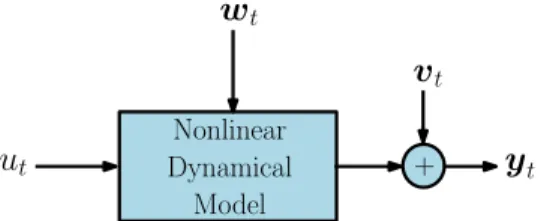
In this thesis, we are concerned with the parameter estimation problem of fairly general stochastic nonlinear dynamical models. We are specifically interested in cases where an unobserved disturbance or latent process is affecting the outputs through a non-invertible nonlinear transformation. This is illustrated in the block diagram in Figure 1.1. We will make the standing assumption that a parametric model set is given and we will not be concerned with the important step of model structure selection. Our objective is to apply either the ML method or a consistent instance of the PEMs.

u

w

v

y

Figure 1.1: A stochastic nonlinear model. The input ut is known and the output

yt is a stochastic process. The disturbance wt is an unobserved stochastic process

affecting the output through the nonlinear dynamics, and vtis an additive measurement

noise. Both wt and vt are usually assumed to be mutually independent and to have

To motivate the problem, we consider below two cases. In the first, the stochastic part of the outputs comes from an additive measurement noise; in this case, the model is invertible in the sense that, for any given θ, the measurement noise can be reconstructed from the knowledge of the inputs and the outputs. In the second, a nonlinear contribution from an unobserved disturbance is also present; in this case the inputs and outputs cannot be used to reconstruct the unobserved disturbance, and the model is said to be non-invertible.

For each case, we provide a very brief overview of the available identification methods. There is a significant literature on this topic, and it is not possible to cover all the relevant work in a brief overview. However, we refer the interested reader to the surveys [12, 57, 126, 128, 134], the books [13, 48, 101, 104, 111], and the exhaustive references lists therein. The Ph.D. theses [36, 87, 127, 132] cover the most recent methods dealing with identification for nonlinear systems.

1.2.1

Case 1: Invertible Models

Consider the static model

y_t= g(ut; θ) + vt, t= 1, 2, 3, . . . (1.1)

with scalar inputs utand outputs yt, in which g(⋅; θ) ∶ R → R is a nonlinear function

parameterized by θ, and for any time t∈ N the random variable vt has a known

PDF, that is vt∼ p(vt). Observe that a bold font is used to denote random variables

and a regular font is used to denote realizations thereof. We assume that vtand vs

are independent whenever t≠ s. Since the input sequence {ut} is known, it is clear

that the outputs are independent over t.

Let us define the vector Yt ∶= [y1 . . . yt]⊺, and let Y ∶= YN. We can easily

construct the joint PDF of the model outputs,

p(Y ; θ) = N ∏ t=1 p(y_t; θ) = N ∏ t=1 pvt(yt− g(ut; θ)), (1.2)

and therefore we have no trouble formulating the ML optimization problem (see Definition 2.4.2): ˆ θML∶= arg max θ N ∏ t=1 pvt(yt− g(ut; θ)).

Because the outputs are independent over time, it is also easy to show, see [92, Chapter 3], that the optimal (mean-square error) one-step ahead predictor is given by

ˆyt∣t−1(θ) ∶= g(ut; θ),

and we can simply define a suboptimal but consistent (see Definitions 2.3.2 and 2.3.3) PEM estimator (see Definition 2.4.4) as the minimizer of an unweighted nonlinear least-squares problem:

ˆ

θPEM∶= arg min θ

N

∑

t=1(y

t− ˆyt∣t−1(θ))2= arg min θ

N

∑

t=1(y

Under some weak conditions on the model, the parameterization and the input signal (see [92, Chapter 8]), it is known that both estimators are consistent and asymptotically normal (see Definition 2.3.4).

We get a direct extension to the dynamic case if we allow the function g to depend on previous inputs and outputs. Most of the classical research found in the literature on nonlinear system identification is dedicated to this case, and generally focuses on two main issues: (i) the problem of model selection and parameterization, and (ii) the optimization methods used to fit the parameters to the data. Most of the work is done using a slightly more general model compared to (1.1) and is given by the equations

y_t= ψ(ϕ(t; θ); θ) + vt, t= 1, 2, 3, . . . (1.3)

The nonlinear mapping ψ is known as the predictor function, and ϕ(t; θ) is a parameterized regression vector that is a function of past inputs, past outputs, and past prediction errors et(θ) ∶= yt− ψ(ϕ(t; θ); θ). Observe that the model in (1.3)

assumes that wt in Figure 1.1 is identically 0 for all t but allows for a recurrent

structure; i.e., the current output may depend on previous inputs and outputs (see [134]). Several possibilities of parameterizing the predictor function and selecting the regressor variables can be found in the above cited books and surveys. For instance, they include Volterra kernel representations, Nonlinear AutoRegressive eXogenous (NARX) models, Nonlinear AutoRegressive Moving Average eXogenous (NARMAX) models, nonlinear state-space models in predictor form, and block-oriented models with only additive measurement noise and no latent disturbances.

The Volterra representation is an example of a nonparametric structure and is described in detail in the book [124]. It can be seen as a generalization of the impulse response of linear models to the nonlinear case. Its identification requires the estimation of the kernels which, according to their orders, might contain thousands of parameters. The recent research effort in [14] applied regularization techniques to Volterra kernels estimation in the hope of improving the accuracy of the estimates for reasonable data sizes.

The NARX and NARMAX models are generalizations of the linear AutoRegres-sive eXogenous (ARX) and AutoRegresAutoRegres-sive Moving Average eXogenous (ARMAX) models defined in [92, Chapter 4]. They are flexible nonlinear model structures that provide input-output representations of a wide range of nonlinear systems including models with nonlinear feedback; they are studied in detail in the book [13]. One of the main advantages of such structures is their parsimony; the dimension of the parameterization vector of a NARX or a NARMAX model is small compared to other available nonlinear models.

Block-oriented models (see [48]) are models consisting of two main block types: static nonlinearity blocks and Linear Time-Invariant (LTI) dynamical blocks. The LTI blocks can be represented by parametric models such as rational transfer operators, linear state-space models, basis function expansions or by nonparametric models in either time or frequency domain. Similarly, the static nonlinearity can be represented by a nonparametric kernel model, or by some linear-in-parameters basis

function model. A block-oriented model structure is developed by connecting several of these two building blocks together in series or in parallel, or both. Feedback connections are also possible. Although not as general as the Volterra representation or the NARMAX models, the block-oriented structures may be used to model many real-life nonlinear systems (see [48]). The simplest block-oriented structures are series connections involving only one block of each type, see Figure 1.2. A Wiener model is constructed by a single LTI block followed by a static nonlinearity block at the output; a Hammerstein model is constructed by a static nonlinearity block at the input followed by an LTI block. The model complexity can be increased by connecting these simple models in series or in parallel as shown in [48].

ut

vt

yt

+ LTI _NonlinearityStatic

(a) Wiener model: an LTI model followed

by a static nonlinearity at the output

ut vt yt + LTI Static Nonlinearity

(b) Hammerstein model: a static

nonlinear-ity at the input followed by an LTI model.

Figure 1.2: A Wiener and a Hammerstein model.

One main advantage of block-oriented structures is the possibility of separat-ing the estimation of the linear and nonlinear parts of the model. Under some assumptions on the input signal and the noise, it is possible to construct best linear approximations (BLA) of the model, see [36, 93, 129, 130], which can be shown to be related to the LTI blocks, see [128, 132]. The main tool there is Bussgang’s theorem given in [18]; it states that the cross-correlation functions of a Gaussian signal before and after passing through a static nonlinear function are equal up to a constant. However, the constant may well be 0 (see Example 4.2.3 on page 102).

The choice among these different representations is usually guided by prior knowl-edge about the underlying system, the intended use of the model, and the available computational resources, among others. The selection of the model structure is fun-damental and is recognized to be the most difficult step in the system identification procedure. Several specialized methods of structure selection for nonlinear models have been developed in both time and frequency domain, see [13] and [128].

The parameter estimation step for the model in (1.3) remains relatively simple. The ML problem can be easily formulated assuming a known distribution for vt

and known initial conditions. Observe that the regression vectors of the NARMAX mode include delayed measurement noise; the NARMAX model is defined by the relations

y_t= ψ(y_t−1, . . . , y_t−ny, ut−1, . . . , ut−nu, vt−1, . . . , vt−nv; θ) + vt, t∈ Z, for some ny, nu, nv∈ N. The values vt−1, . . . , vt−nv can be evaluated using the model, the initial conditions and the previous inputs and outputs (it is an invertible model). This allows us to compute the likelihood function in closed-form. Similarly, it is

still possible to formulate a PEM problem in closed-form. A PEM estimator can be defined, for example, as the global minimizer

ˆ θ∶= arg min θ∈Θ N ∑ t=1 ∥yt− ψ(ϕ(t; θ); θ)∥ 2_.

Depending on the parameterization of the predictor function and the regression vector, the solution is usually not available in closed-form. The resulting optimization problem is in general non-convex. Nonlinear optimization algorithms like the damped Gauss-Newton algorithm or the Levenberg-Marquardt algorithm (see [42, 104, 108]) are therefore required. These algorithms are numerical iterative methods that can only find a local minimum. They require a good initial value to guarantee that the solution is in the vicinity of a global minimizer. In the case of block-oriented models, linear approximations can be used to initialize the optimization algorithms. There have been some research efforts in this direction, see for example [97, 110, 132, 133, 135, 136]. However, it should be noted that the problem of finding a linear approximation, depending on the chosen model structure for the LTI blocks, might still be a difficult non-convex problem.

To avoid possible local minima for complicated parameterizations, it is also possible to use random global search strategies such as simulated annealing and genetic algorithms (see [104, Chapter 5] or [117, Chapter 5]). However, due to their random nature, the exploration of the entire optimization domain could be computationally expensive and time-consuming. On the other hand, several approaches constrain the possible parameterization of the model in such a way that the resulting optimization problem has a closed-form solution (for example considering only linear-in-parameters models (see [134, Section 8] or [13, Chapter 3]).

The model in (1.3) ignores any possible stochastic process (different from vt) that

passes through the nonlinear dynamics. This is an idealization of the real situation where there might exist a disturbance entering the system before some nonlinear subsystem. It has been shown in [58] that if the process disturbance is ignored, the resulting estimators will not be consistent. Therefore, it is important to develop identification methods that take into account the presence of such disturbances, which is the aim of this thesis.

1.2.2

Case 2: Non-invertible Models

Assume that the output does not only depend on the input and the variables vt,

but also on some (latent) unobserved process wtthrough a non-invertible (in wt)

nonlinear function. In this case, the output becomes

yt= g(wt, ut; θ) + vt, t= 1, 2, 3, . . . (1.4)

in which g(⋅, ⋅; θ) ∶ R × R → R is a non-invertible (w.r.t. wt) nonlinear function

Define the vector Wt ∶= [w1 . . . wt]⊺, let W ∶= WN, and assume that

W ∼ p(W ; θ) which has a known functional form. Let us first consider the ML problem. Note that the outputs are independent only if the latent process w is independent over. We also observe that because W is not observed, the PDF of Y has to be calculated by marginalizing the joint distribution p(Y , W ; θ) with respect to W ; that is

p(Y ; θ) = ∫

Rdw N

p(Y , W; θ) dW. (1.5)

Unfortunately, even though the integrand in (1.5) has a known form, the integral is a multidimensional integral over RdwN which, in general, has no closed-form expression. The symbol dwdenotes the dimension of the latent process w, which is

assumed to be a scalar process in the current example (i.e., dw= 1). For commonly

encountered models and applications, the value of dwN isO(103) or O(104) and

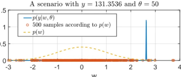
the evaluation of the integral in (1.5) is very challenging due to the nature of the integrand. To be able to find an approximate solution to the ML problem, one has to come up with computational methods that can approximate the maximizer of the intractable function p(Y ; ⋅) over a given set Θ.

Currently, there is an ongoing research effort in this direction within the system identification community; see for example [86, 106, 125, 146, 147] for ML estimation based on sequential Monte Carlo (SMC) methods. The survey [126] summarizes the available state-of-the-art algorithms and distinguishes between two main approaches: (i) the marginalization approach, and (ii) the data augmentation approach.

In the marginalization approach, SMC filters and smoothers (also known as particle filters) are used to “marginalize out” the latent process to approximate the logarithm of the likelihood function (the log-likelihood) and its gradient at a given value of θ. The resulting approximations are then used within an iterative numerical optimization algorithm to find an approximate solution to the ML problem. In the data augmentation approach, the SMC filters and smoothers are used in conjunction with the Expectation-Maximization (EM) algorithm (see [29] or Section 3.2.1) to approximate the MLE as suggested in [144]. The resulting Monte Carlo EM (MCEM) algorithm converges only if the number of the Monte Carlo samples (particles) grows with the algorithm iterations, see for example [20, 43]. Furthermore, a new set of particles has to be generated at each iteration of the algorithm. In order to make a more efficient use of the particles, [28] suggested the use of a stochastic approximation version of the EM algorithm (SAEM) which replaces the expectation step of the EM algorithm by one iteration of a stochastic approximation procedure. In [86], a particle Gibbs sampler (conditional particle filter with ancestor sampling, see [85]) is used within the SAEM algorithm to generate the required particles.

We note here that the available convergence proofs of the MCEM and the SAEM algorithms (see [28, 43]) are, so far, given for cases where p(Y , W ; θ) belongs to the exponential family (see [123, Section 2.2] for a definition of the exponential family). This constrains the distributions of w and v as well as the parameterization of the model.

Estimation methods based on SMC approximations can be computationally expensive. For example, the convergence of the MCEM and the SAEM algorithms can be very slow when the variance of the latent process is small. Furthermore, cases with small or no measurement noise are considered challenging for SMC methods. Moreover, due to the sample degeneracy and impoverishment problems – a pair of fundamental difficulties of SMC methods (see [32, 33]) – the SMC methods are so far, to the best of the author’s knowledge, applicable to models with relatively small

dw.

In this thesis, the ultimate goal is the construction of consistent estimators of θ; we will be looking at alternative approximation methods that can be used to approximately solve the MLE problem without relying on an exact filtering or smoothing distribution. Instead, we only use the parameterized model which defines the joint PDF p(Y , W ; θ). It is of interest to know if this point of view could lead to some computational advantage. We shall deal with this problem in Chapter 3.

The computation of the PEM estimator, for cases with non-invertible model, is not easier than the computation of the MLE. Observe that any estimator ignoring w, as shown in [58], is not guaranteed to be consistent. So far, the available PEMs have relied on approximations of the optimal predictor. The optimal (mean-square error) one-step ahead predictor depends on the history of the observed outputs and is given by the conditional mean (see Chapter 2, page 34),

ˆ

y_t∣t−1(θ) ∶= E[y_t∣Yt−1; θ] = ∫ Rdy

ytp(yt∣Yt−1; θ) dyt, t= 1, 2, 3, . . . (1.6)

in which p(yt∣Yt−1; θ) is known as the predictive PDF and Y0 is defined as the

empty set; hence ˆy1∣0(θ) is constant and is equal to the expectation of y1. Unlike

the MLE, the integrals appearing in the PEM objective function are of the same dimension as that of the output signal. This means that the domain of the integrand is independent of N. For single-input single-output models (like the model in (1.4)), these are one-dimensional integrals; however, the integrand has an unknown form. Unfortunately, to be able to calculate the predictive PDF, we need to compute multidimensional integrals. Observe that by Bayes’ theorem (see [64, page 39]),

p(yt∣Yt−1; θ) = p(Yt; θ) ∫Rdyp(Yt; θ) dyt = ∫Rdw tp(Yt, Wt; θ) dWt ∫Rdy∫Rdw tp(Yt, Wt; θ) dWtdyt . (1.7)

It appears that the predictive PDF of the output depends on p(Yt; θ) which does not

have a closed-form expression. To be able to formulate and solve a PEM problem, one has to come up with either consistent instances of the PEMs without relying on the optimal predictor, or computational methods that can approximate the conditional mean (1.6). In the latter case, it seems that the PEM does not have any computational advantage over the efficient ML method. Both the MLE and the conditional mean of the outputs require the solution of similar marginalization integrals. For this reason, most of the recent research efforts found in the system identification literature, so far, target the maximum likelihood estimator.

One of the main contributions of this thesis is the introduction of one-step ahead predictors constructed using the postulated statistical model without any reference to the data or the the likelihood function (see Chapter 4). These predictors are relatively easy to compute and the can be used to construct consistent instances of the PEMs. The predictors do not necessarily coincide with the optimal predictor, which means that certain asymptotic properties (such as statistical efficiency) cannot be guaranteed. However, the introduced predictors are algorithmically and conceptually simpler than predictors based on either SMC smoothing algorithms or Markov Chain Monte Carlo (MCMC) algorithms.

The main challenge

The two cases discussed above clarify the source of difficulty of the estimation prob-lems considered in this thesis. The difference between the “tractable” model in (1.1) and the “intractable” model in (1.4) is the non-invertible nonlinear transformation of unobserved random variables in the latter. This makes the likelihood function and the optimal one-step ahead predictor of the output analytically intractable. Consequently, the objective functions of the optimization problems of both the MLE and the PEM estimator are not available in closed-form.

1.3

Thesis Outline and Contributions

The content of this thesis concerns the estimation problem of parametric nonlinear stochastic dynamical models. Firstly, several possible approximations of the MLE are explored. Secondly, computationally attractive PEM estimators based on non-stationary linear one-step ahead predictors are introduced. Below, an outline of each chapter is given where we also indicate the main contributions.

Chapter 2: Background and Problem Formulation

Chapter 2 provides the necessary background for the thesis. Here, several important remarks and observations are made. After introducing a stochastic framework, a classical result on the structure of general second-order stochastic processes – due to Harold Cram´er in [27] – is introduced. It generalizes Wold’s decomposition (see [148]) of stationary processes by giving an exact description of the second-order properties of a non-stationary process in terms of a causal “linear” time-varying filtering of the innovation process. This interesting result is used in Chapter 4 as the basis for optimal linear prediction of non-stationary processes with nonlinear underlying models. The chapter also introduces two frequentist estimation methods: the ML method and the PEMs based on PE minimization. The kinship between the two methods is highlighted using linear dynamical models. Finally, the main problem of the thesis is formulated.

Chapter 3: Approximate Solutions to the ML problem

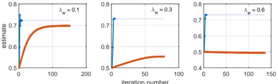
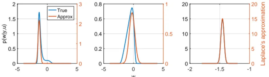
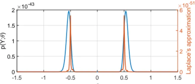
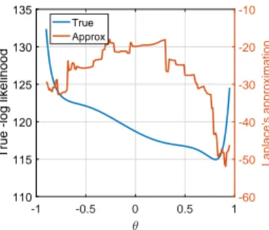
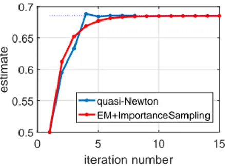
In this chapter, we investigate several approaches to approximate solutions of the ML estimation problem. The focus is on the EM algorithm and the quasi-Newton algorithm. For both algorithms, analytical as well as numerical approximations are explored. The analytical approximations are based on a Gaussian approximation of the posterior of the unobserved (latent) disturbance (using Laplace’s method). The numerical approximations, in cases where the output process is independent, may be obtained by using deterministic integration; however, in general, Monte Carlo approximations based on importance sampling are considered. The performance of the approximate algorithms is evaluated on several (relatively simple) numerical examples where the advantages and disadvantages of each method are highlighted. The material in this chapter has not appeared in any publications, except the last part of Section 3.4.2 concerning Monte Carlo approximations of the quasi-Newton algorithm based on Laplace importance sampling (Algorithm 3.4.2); this algorithm has been published in

Mohamed Abdalmoaty and H˚akan Hjalmarsson. A Simulated Maximum Likelihood Method for Estimation of Stochastic Wiener Systems. In the 55th

IEEE Conference on Decision and Control (CDC), pp. 3060-3065, Las Vegas,

USA, 2016

Chapter 4: Linear Prediction Error Methods

In this chapter, we propose a relatively cost-efficient PEM based on suboptimal predictors. The used predictors are defined using only the first two moments of the postulated model; they are linear in the observed outputs, but are allowed to depend nonlinearly on the (assumed known) inputs. The optimal linear predictors, in the sense of minimum mean-square error, are derived and used to construct a PEM estimator. It is shown that for several relevant models with intractable likelihood functions (such as stochastic Wiener-Hammerstein models with polynomial nonlinearity), the suggested PEM estimators are defined by closed-form (exact) expressions. Under some mild assumptions, the resulting estimators are shown to be consistent and asymptotically normal. The chapter also discusses the relation between the proposed PEMs and a suggested approximation in Chapter 3. We give the PEM a maximum likelihood interpretation that allows for the use of the EM algorithm. The performance of the method is illustrated by numerical simulations using several challenging models. Finally, a comparison and a connection are made to a PEM based on the Ensemble Kalman filter – a Monte Carlo filter used to define a (nonlinear) suboptimal predictor.

The ideas developed in this chapter have originated in

Mohamed Abdalmoaty and H˚akan Hjalmarsson. Simulated Pseudo Maximum Likelihood Identification of Nonlinear Models. In IFAC-PapersOnLine, Volume 50, Issue 1, pp. 14058–14063, 2017.

Chapter 5: Conclusions and Future Research Directions

In this last chapter, we summarize the conclusions of the thesis and give some pointers for future research.

Appendices

The thesis contains three appendices where relevant definitions and results are summarized. Appendix A introduces the idea of Monte Carlo estimation. Random sampling, common random numbers, and importance sampling are defined and discussed. In Appendix B, Hilbert spaces of random variables are defined and the optimal linear mean-square error predictors are derived based on the projection theorem. Lastly, Appendix C gathers some relevant properties of Gaussian random vectors and multivariate Gaussian distributions.

Background and Problem Formulation

2.1

Mathematical Models

The mathematical models considered in this thesis belong to the set of stochastic models; all the signals are modeled using stochastic processes. A stochastic process y = {y_t ∶ t ∈ T} is a family of random variables indexed by a given index set

T and defined over a common underlying probability space (Ω, F, Pθ). In this

thesis, the probability measure is parameterized by a finite-dimensional real vector

θ∈ Θ ⊂ Rd _{for some d∈ N. The index t always refers to time and the index set T}

is taken as the set of integers Z giving rise to discrete-time stochastic processes (a classical reference on the theory of stochastic processes is [31]). For any finite subset{t1, . . . , tN} ⊂ Z, the joint distribution of the random variables {yt1, . . . , ytN} is known as a finite-dimensional distribution of the process. For every t, we always assume the existence of a joint probability density function p(Yt; θ) of the vector

Yt∶= [y⊺1, . . . , y ⊺ t]

⊺. The probability measure P

θ can be characterized by specifying

the finite-dimensional distribution for all finite subsets of Z. The mathematical models are then deterministic objects that define the probability measure Pθ on the

space of observed signals. Because all practical systems are causal systems, for which the current output does not depend on the future inputs or future disturbances, we limit ourselves to causal models. We start by defining special classes of signals.

2.1.1

Signals

The outputs, inputs, and disturbances are modeled using stochastic processes. The mathematical models to be developed are deterministic functions that define a

mapping between these processes. We will only consider dζ-dimensional real-valued

second-order discrete-time stochastic processes ζ with some finite dζ∈ N.

Definition 2.1.1 (Second-order discrete-time stochastic process). A stochastic

process y= {yt∶ t ∈ Z} is said to be a second-order stochastic process if it holds that

E_{[yt] = µt}, ∥µt∥ ≤ C < ∞, ∀t ∈ Z,

E_[yty⊺

s] = Ry(t, s), ∥Ry(t, s)∥ ≤ C < ∞, ∀t, s ∈ Z

where C is a generic constant (that does not necessarily assume the same value when bounding different quantities).

One of the simplest and most used classes of second-order stochastic processes is the class of stationary processes.

Definition 2.1.2(Stationary discrete-time stochastic process). A stochastic process y= {y_t∶ t ∈ Z} is strictly stationary if for any {t1, . . . , tN} ⊂ Z, the joint distribution of the random variables{y(t1+ τ), . . . , y(tN+ τ)} is independent of τ.

It is weakly stationary, or wide-sense stationary, if it holds that

E_{[yt] = µ ∀t ∈ Z,} E_{[(yt− µ)(yt+τ− µ)}⊺] = R

y(τ) ∀τ ∈ Z.

A weaker concept of stationarity, commonly used in system identification (specif-ically when LTI models are used), is quasi-stationarity. It allows for a common framework for stochastic and deterministic signals, and is used to imply that the signals satisfy regularity conditions (a form of ergodicity) used for the asymptotic analysis of the identification methods.

Definition 2.1.3(Quasi-stationary stochastic process [92, Section 2.5]). A

stochas-tic process y= {yt∶ t ∈ Z} is quasi-stationary if

E_{[yt] = µt}, ∥µt∥ ≤ C, ∀t ∈ Z, E_[yty⊺ s] = Ry(t, s), ∥Ry(t, s)∥ ≤ C, ∀t, s ∈ Z, lim N →∞ 1 N N ∑ t=1 Ry(t, t − τ) = Ry(τ), ∀τ ∈ Z,

in which the expectation operator is with respect to the distribution of the random component of the signal. If the signal is deterministic, then the expectation operator can be omitted.

A special class of second-order stochastic processes is the class of white noise processes.

Definition 2.1.4 (White noise). A stochastic process ζ= {ζt∶ t ∈ Z} is white noise if E[ζt] = 0, ∥E[ζtζ

⊺

t]∥ < ∞ ∀t ∈ Z, and E[ζtζ ⊺

s] = 0 ∀t ≠ s. In words, white noise is a sequence of uncorrelated random variables with zero mean and finite second order moments.

This definition of white noise is “weak” and is used when the estimation method does not rely on the exact distribution of the process, but only on the first and second moments. In this case, the exact finite-dimensional distributions of the process are not specified. However, it is sometimes required to work with white noise which is a sequence of independent random variables; in this case, we speak of an independent process (or independent white noise). Furthermore, in some cases, it is assumed that the white noise is an independent and identically distributed (i.i.d.) process (following a Gaussian distribution for example).

In system identification, the disturbances (uncertain errors) are usually under-stood to come from two main sources. The first source is the imperfections of the sensing devices used to measure the outputs; this is known as measurement noise. The second source is the uncontrollable inputs (passing through the system) that affect the observed outputs; this is known as process disturbances. In the linear setting, the measurement noise is commonly assumed to be white noise, while the process disturbances are usually modeled as linearly filtered white noise. The inputs are normally assumed to be known deterministic signals or known realizations of stochastic processes; in either case, it is usually assumed that the input is quasi-stationary. Under some assumptions on the data-generation mechanism, it is possible to show that the output is also a quasi-stationary signal.

A mathematical model in this thesis is understood to be the rule that specifies the evolution of the signals through time. In other words, it is the deterministic structure underlying the stochastic observations. A relevant result that gives interesting insights regarding the structure of certain classes of stochastic processes is Wold’s decomposition introduced in [148] and its extension in [27].

Wold’s decomposition

Consider a vector-valued discrete-time stochastic process y∶={yk}∞k=−∞⊂L n

2(Ω, F, Pθ).

Here, the space Ln

2(Ω, F, Pθ) is the Hilbert space of random variables, with zero

mean and finite covariance, defined over(Ω, F, Pθ) and assuming values in Rn (see

Appendix B). In what follows, we will be referring to this space simply as Ln 2.

Define the Hilbert spaces

Ht∶= sp{ys∶ s ≤ t}, ∀t ∈ Z (2.1)

in which the symbol sp{S} is used to denote the closure of the span of S ⊂ Ln 2.

Observe that we can always project ytonto Ht−1 and define the difference

εt∶= yt− PHt−1[yt] (2.2)

in which P denotes the projection operator (see Appendix B). The vector εt is

known as the innovation in yt and is orthogonal to Ht−1 by construction. The

process ε is known as the “innovation process” of the process y (the name was suggested in [27]).

Definition 2.1.5(The (linear) innovation process). The stochastic process defined

by

εt∶= yt− PHt−1[yt], yt∈ L n

2, ∀t ∈ Z

is called the innovation process of y. If it holds that E[εtε⊺t] ≻ 0 ∀t ∈ Z (i.e. the covariance matrix of εt is positive definite), then the process y is said to be full rank.

By the definitions (2.1), (2.2), and the properties ofP, it holds that PHt−1[yt] = P{εt−1}[yt] + PHt−2[yt]

and therefore we may write

y_t= εt+ P{εt−1}[yt] + PHt−2[yt], t ∈ Z.

Because ε has the same dimension as y andP is, by definition, a linear operator, it holds that

P{εt−1}[yt] = h1(t)εt−1

in which h1(t) is a square matrix of real numbers. We can repeat the above projection

mtimes and write

y_t=

m−1

∑

k=0

hk(t)εt−k+ PHt−m[yt] (2.3) in which h0(t) = I. Now notice that the variance of the first term on the right hand

side of (2.3) increases with m but is bounded by the variance of yt. Due to the

orthogonality of the two terms, the variance of the second term decreases with m and is nonnegative. Therefore, asymptotically in m we have

y_t= ∞ ∑ k=0 hk(t)εt−k+ ydt = Ht(q)εt+ ydt, t∈ Z (2.4) where{hk(t)Σt−k}∞k=0 is a square summable sequence. The representation of y in

(2.4) is known as Wold’s decomposition. Here, Σt−k is a square root of E[εt−kε⊺t−k], Ht(q) = ∑

∞

k=0hk(t)q−k is a monic linear time-varying transfer operator (see Section

2.1.3) and yd

t ∈ Ht−m for all m∈ N. This last observation means that ydt can be

predicted perfectly given the historyHt−m (i.e.,{yk}t−mk=t−∞), regardless of the value m. For this reason, the stochastic process yd _{is called the linear deterministic part}

of y. When this part is zero, the process y is known as a purely non-deterministic stochastic process and it can always be written as the output of a causal linear time-varying filter excited by white noise

y_t= Ht(q)εt= εt+ ∞

∑

k=1