J
Ö N K Ö P I N GI
N T E R N A T I O N A LB
U S I N E S SS
C H O O LJÖNKÖPI NG UNIVER SITY
T h e R e l a t i o n s h i p B e t w e e n S w e d i s h
E q u i t y F u n d s ’ M a n a g e m e n t Fe e s
a n d Pe r f o r m a n c e
Bachelor thesis within Financial Economics Author: Emil Abona, 831010
Tutors: Prof. Ulf Jakobsson Ph.D. Daniel Wiberg Jönköping May 2007
Bachelor Thesis within Financial Economics
Title: The Relationship Between Swedish Equity Funds’ Man-agement Fees and Performance
Author: Emil Abona
Tutors: Prof. Ulf Jakobsson
Ph.D. Daniel Wiberg
Date: April 2007
Subject terms: Financial Economics, Equity Fund, Management Fees
Abstract
An increasing number of people in Sweden and in the rest of the world are becoming more interested in the mutual fund sector. Investments in mutual funds have grown rapidly these past few years. Nilsson (2004) wrote that 85 percent of the Swedish population invested in mutual funds in 2004. The Swedish Investment Fund Association also found an increase in investments in mutual funds; 83 billion Swedish crowns were invested in mutual funds in 2005, an increase from 56 billion in 2004.
The purpose of this thesis is to evaluate whether or not there is a relationship between low fee, middle fee, and high fee charging Swedish Equity funds and their respective perform-ance (unadjusted and risk-adjusted returns).
The Modigliani & Modigliani (1997) risk-adjusted performance measurement was used to calculate the risk-adjusted performance of the 130 mutual funds. And the linear regression was used to analyze whether or not there was a relationship between the variables (man-agement fee vs. returns/risk-adjusted returns). The mutual funds were also divided into three different categories, based on their management fees; low, middle and high fee mu-tual funds.
The analysis illustrated that there was no clear relationship between the management fee and the returns/risk-adjusted returns. There was some connection found between the management fee and the low, middle fee category. However, this research confirms that in-vestors should not believe that a mutual fund which charges higher fees necessarily gener-ate higher returns.
Kandidatuppsats inom Finansiell Ekonomi
Titel: Relationen mellan Globala Svenska Fonders Förvaltnings-avgift och deras Prestanda
Författare: Emil Abona
Handledare: Prof. Ulf Jacobsson Ph.D. Daniel Wiberg
Datum: April 2007
Ämnesord: Finansiell Ekonomi, Aktiefonder, Förvaltnings avgift
Sammanfattning
Fler och fler människor blir mer intresserade av att investera i fondindustrin. Investeringar i fond sektorn har ökat starkt de senaste åren. Nilsson (2004) skrev att 85 procent av den svenska befolkning hade investerat i fonder under år 2004. Fondbolagens förening fann en ökning av i investeringar i fonder; 83 miljarder SEK hade investerats i fond industrin, detta var en ökning med 56 miljarder från 2004.
Syftet med denna uppsats var att undersöka ifall det finns något samband mellan låg, medel och hög kostnads Aktiefonder och deras respektive avkastning/riskjusterade avkastning. Modigliani & Modigliani’s (1997) riskjusterade avkastningsmodell användes för att räkna ut den riskjusterade avkastningen på de 130 svenska fonderna. En linjär regression användes för att analysera om det fanns ett samband mellan de olika variablerna (förvaltnings avgift vs. Avkastning/riskjusterad avkastning). Fonder delades upp i tre olika kategorier, baserat på deras respektive avgifter; låg, mellan och hög kostnads fonder.
Utvärderingen av Aktiefonderna visade att det inte fanns ett uppenbart samband mellan förvaltningsavgiften och avkastningen/riskjusterade avkastningen. Det fanns ett svagt sam-band mellan förvaltningsavgiften och de låg och mellan avgifts fonderna. Uppsatsen styrker att investerare inte skall tro att en fond som debiterar högre avgifter nödvändigtvis generera högre avkastning.
Table of Contents
1
Introduction ... 1
1.1 Background...1
1.2 Purpose ...1
1.3 Chapter Outline...1
2
Risk and Return ... 2
2.1 Modern Portfolio Theory ...2
2.2 Return on Investments ...2
2.2.1 Arithmetic Average Return on Investments ...3
2.2.2 Criticism of the Return on Investments...3
2.3 Risk of Investments...4
2.3.1 Standard Deviation ...4
2.3.2 Criticism of the Standard Deviation ...5
2.3.3 Tracking Error ...5
3
Risk-Adjusted Performance and the Attributes of Mutual
funds ... 5
3.1 The Risk-Adjusted Performance of Mutual Funds...5
3.2 The Capital Asset Pricing Model ...6
3.3 The Sharpe Ratio ...6
3.4 The M2 - measure ...7
3.5 Attributes of Mutual Funds ...7
3.5.1 The Management Fee ...7
3.5.2 What is included in the Management Fee? ...8
4
Earlier Studies and Hypothesis ... 8
4.1 Hypothesis...9
5
Method and Data ... 9
5.1 Statistical Method ...9 5.2 Data...10
6
Empirical Results ... 10
6.1 Descriptive Statistics...11 6.2 Results ...11 6.2.1 Regression 1 & 2...11 6.2.2 Regression 3 & 4...137
Discussions... 14
7.1 Regression 1 & 2...14 7.2 Regression 3 & 4...158
Conclusion... 16
8.1 Further Studies ...17References ... 18
Figures
FIGURE 1–RETURN &RISK...4
Tables
TABLE 6-1–DESCRIPTIVE STATISTICS (2003-2005) ...11TABLE 6-2–REGRESSION 1:MANAGEMENT FEE VS.TOTAL AVERAGE RETURN (2003-2005) ...12
TABLE 6-3–REGRESSION 2:MANAGEMENT FEE VS.TOTAL AVERAGE RETURN (2003-2005) ...12
TABLE 6-4–REGRESSION 3:MANAGEMENT FEE VS.RISK-ADJUSTED RETURN (2003-2005)...13
TABLE 6-5–REGRESSION 4:MANAGEMENT FEE VS.RISK-ADJUSTED RETURN (2003-2005)...14
Equations
EQUATION 1:RETURN ON INVESTMENTS...2EQUATION 2:ARITHMETIC AVERAGE RETURN ON INVESTMENTS...3
EQUATION 3:STANDARD DEVIATION...4
EQUATION 4:SHARPE RATIO...6
EQUATION 5:M2–MEASUREMENT...7
1
Introduction
1.1
Background
For decades investors have been trying to come up with a trading strategy that could out-perform the market. Investors are more interested today than they have ever been in evalu-ating the performance of their securities; mutual funds, stocks, bonds etc.
When investing on the stock market, it is important for investors to diversify their invest-ments. This can be done by either investing in many different stocks or investing in mutual funds (which is a portfolio with many different securities). This will decrease the risk of the investment.
In Sweden the mutual fund sector has grown rapidly these past few years, according to Nilsson (2004) 85 percent of the Swedish population invested in mutual funds in 2004. The Swedish Investment Fund Association also found an increase in investments in mutual funds; 83 billion Swedish crowns were invested in mutual funds in 2005, an increase from 56 billion in 2004.
Many researchers have presented their theories about mutual fund performance evaluation. To name a few of them; Sharpe, Treynor, Modigliani and many more have tried their luck with evaluating the mutual fund industry. Before these theories were presented by Sharpe, Treynor etc., mutual funds were evaluated by comparing the total returns of a managed portfolio with those of unmanaged portfolios chosen at random.
When evaluating mutual funds one has to consider fund attributes, such as the manage-ment fees that are paid by the investors to the fund managers to manage their investmanage-ments. When a person wants to buy a certain product or service, he/she weights in the costs of the actual purchase and so do investors when they buy their mutual funds. They consider how much they want to pay for this investment and whether it is worth the costs.
1.2
Purpose
The purpose of this thesis is to evaluate whether or not there is a relationship between low fee, middle fee, and high fee charging Swedish mutual funds and their respective perform-ance (unadjusted and risk-adjusted returns).
This thesis will investigate whether or not there is a stronger connection between the re-turns and the management fee of high fee funds, because if an investor is charged by a higher fee from a fund company then he/she expects higher returns.
1.3
Chapter Outline
Chapter one in this thesis will introduce the reader to the subject and present the purpose of this research. Further down in chapter two is where you can find the risk and return chapter which are the fundamental theories in this thesis.
Chapter three and four will describe the different theories used to calculate the risk-adjusted performance and also present attributes of mutual funds. However, focusing more on the management fees. Chapter five will present the hypothesis testing and some earlier studies conducted in the same field of research to connect them to the results of this study.
Chapter six will present the methods and data used to evaluate the mutual funds in this thesis. While the empirical results in chapter seven present the results retrieved from a lin-ear regression analysis.
Chapter eight will discuss and analyze the empirical results and also test the hypothesis and connect them to earlier studies to observe whether there are some similarities. The conclu-sion is presented in chapter nine and also some thoughts about future studies in the same field.
2
Risk and Return
Investors are in general very interested in getting the correct information in order to make the correct choices before investing their money in stocks, bonds, mutual funds etc. Many studies have been performed during these past decades to evaluate the mutual fund markets around the world. However, most studies are of US fund data, which have found that cash flows, returns and fees can be used when evaluating future mutual fund perform-ance.
2.1
Modern Portfolio Theory
When a person constructs a portfolio of assets, he/she often seek to maximize the ex-pected return from their investment given some level of risk they are willing to accept. Portfolios that satisfy this requirement are called “efficient portfolios” (Fabozzi &
Modi-gliani & Ferri 1994).
Harry Markowitz was first to develop the “portfolio theory” or the “Modern portfolio the-ory”. It was first published in the Journal of Finance in 1952. The theory was based on the assumptions that an investor should choose to construct a portfolio which is composed by different stocks moving in the opposite direction in the market, where the most efficient way to reduce risk occurs when two stocks are negatively correlated.
To construct an efficient portfolio, it is necessary to understand what is meant by “ex-pected return” and “risk” (Fabozzi & Modigliani & Ferri 1994).
This chapter deals with the return on investments to illustrate how to calculate the returns on investments. It is also illustrated further down how an investor can calculate and inter-pret the risk of a security.
2.2
Return on Investments
Investors invest their capital on the financial markets to try to generate the highest returns. The returns on an investor’s portfolio during a given time interval is equal to the change in value of the portfolio plus any dividends received from the portfolio, expressed as a frac-tion of the initial portfolio value. It is important that any capital or income distribufrac-tions made to the investor is to be included, or the measure of return will be deficient. The re-turn on the investor’s portfolio, RP, is given by:
Equation 1: Return on Investments
RP = (P1 – P0+ D1) / P0) Where,
P0 = The portfolio market price at the beginning of the interval D1 = The cash distributions to the investor during the interval
According to Fabozzi, Modigliani and Ferri (1994) the RP assumes that any interest or divi-dend income received on the portfolio of securities and not distributed to the investor are reinvested in the portfolio (and thus reflected in P1). Further the calculation assumes that any distributions occur at the end of the interval, or are held in the form of liquid assets un-til the end of the interval. If the dividends were reinvested prior to the end of the interval, the calculation would have to be changed to consider the gains or losses on the amount re-invested. The measurement also assumes no capital inflows during the interval. Otherwise, the calculation would have to be modified to reflect the increased investment base. Capital inflows at the end of the interval (or held in cash until the end), can be treated as just the reverse of distributions in the return calculation.
2.2.1 Arithmetic Average Return on Investments
The arithmetic average return on investments is an unweighted average of the returns achieved during a series of such measurement intervals. The general formula is:
Equation 2: Arithmetic Average Return on Investments
RA = (Rp1 + R p2+……+ R pN) / N RA RA = The arithmetic average return
R pK = The portfolio return in interval K as measured by equation 1, K = 1,…., N Of intervals
N = Number of intervals in the performance evaluation period
2.2.2 Criticism of the Return on Investments
The return on investments can be calculated in any time period, for one month or ten years. However, some researchers have criticized the measurement because they claim that calculations made over a long period of time would not be very reliable since of the as-sumptions that all cash payments and inflows are made and received at the end of the pe-riod. Another problem that the return on investments measurement face is that, one can-not rely on the calculations to compare return on a one-month investment with that on a ten-year portfolio. To use the return on investments to compare different portfolios, the portfolio should then be expressed per unit of time, e.g. a year.
2.3
Risk of Investments
Investors are fond of high returns and less fond of risk. Each investor has his/her limits as of how much risk they can bare to take. Most in-vestors are more sensitive to increased risk than increased return. Padgette (1995) wrote that all investments includes risk, whether you are investing in stocks, bonds or any kind of security, you have to deal with the fact that you can make a loss instead of a gain. The higher the
return you are striving for the higher the risk will be (fig. 1).
According to Simons (1998) investors are not only interested in mutual fund returns; they are also interested in risks which are taken to achieve those returns. People think of risk as the uncertainty of the expected return, and uncertainty is generally equated with variability. Investors demand and receive higher returns with increased variability, suggesting that vari-ability and risk are related.
2.3.1 Standard Deviation
The Standard deviation measurement is probably used more often than any other meas-urement to estimate a mutual fund’s risk. It is a statistical measmeas-urement used to define the scattering of returns around the average return. The method is also often used to define uncertainty of an outcome and used in the evaluation of investments for the same purpose. An investment with a low standard deviation is less “risky” than an investment with a higher standard deviation (Padgette, 1995).
Equation 3: Standard Deviation
σi = √ (Σi-1 (TRi – AR)2 / (n-1)) where, σi = Standard Deviation.
TRi = Total return during period i AR = Average return during n periods n = Time period
The standard deviation is often used since it provides an accurate measure of how different a fund's returns have been over a particular time period. This calculation can give a prob-ability of the returns the fund is likely to generate in the future. If the returns of a mutual fund rose by 1 percent each and every month for the next 36 months it has a standard de-viation of zero, since the returns did not change during that time period. However, if the returns of a fund increased by 5 percent one month, 25 percent the next and decreased 7 percent the next, then it would have a high fluctuation and thus a higher standard deviation (Morningstar).
2.3.2 Criticism of the Standard Deviation
Using standard deviation as a measurement of risk can have its negative effects. Mutual funds with a low standard deviation tend to lose less money over short time periods than those with high standard deviations. To make the measurement more useful, it is suggested that the standard deviation of a fund should be compared with similar funds, those in the same category as the fund you are investing in.
2.3.3 Tracking Error
Another method used to estimate risk is to use the tracking error, which calculates weather or not a portfolio might under perform a relevant benchmark. More explicitly, the tracking error measures the expected distribution of a portfolio's return centred on the benchmark's return. It is usually expressed as an annualised standard deviation in percentage terms. It is completely assuming that the distribution of returns is normal, which means that the stan-dard deviation can be transformed into a probability (Lawton-Browne, 2001).
According to Frino & Gallagher (2002) there are a number of different ways of measuring the tracking error. These are:
• The average of the absolute difference in returns between the fund and the bench-mark
• The standard deviation of return differences between the fund and the benchmark • The standard error of a regression of fund returns on benchmark returns
An example of how the tracking error risk works is for instance if a fund’s tracking error is 3.0 percent, the cumulative standard normal distribution tells us that the probability of the portfolio return being within a band stretching from -3.0 percent to +3.0 percent (i.e. one standard deviation on either side of zero) relative to the benchmark return is 66 percent. This means that you expect to outperform by more than 3 percent with a probability of about 17 percent (Lawton-Browne, 2001).
The tracking error was not used in the calculations of the results in this thesis due to the fact that only standard deviation was need for the calculations. The tracking error is pre-sented as an alternative way to calculate the risk of a security.
3
Risk-Adjusted Performance and the Attributes of Mutual
funds
3.1
The Risk-Adjusted Performance of Mutual Funds
This chapter will clarify the risk-adjusted performance measurement used to evaluate the 130 globally operating mutual funds over the period of 2003-2005.
If a stock or a fund has performed well in the past it does not necessarily mean that it will perform well in the future. Often the first thing that an investor looks at is the past per-formance before deciding if he/she will invest in that security or not, though, it is impor-tant to look at what is risked to achieve that performance.
There are many ways of measuring the risk-adjusted performance of a security. Methods that are often used when evaluating mutual funds are the Sharpe ratio and the Capital Asset
Pricing Model. However, this research focuses entirely on Modigliani and Modigliani’s Risk-Adjusted Performance measurement.
3.2
The Capital Asset Pricing Model
Sharpe’s (1964), Treynor’s (1961) and Lintner’s (1965) Capital Asset Pricing Model (CAPM) extended the Markowitz theory to an equilibrium theory. The model is often used as a technique for evaluating financial assets and risk premium. It is used when construct-ing portfolios, measurconstruct-ing performance of investment managers, and valuatconstruct-ing companies etc. The risk in CAPM is generally referred to as beta. Given the risk-free rate and the beta of an asset, one can predict the expected risk premium for that asset (Dhankar, 2005). The Capital Asset Pricing Model assumes that the investors are risk averse and that they have identical preferences about risk and return; risk and return is the only thing they are interested in. The CAPM assumes that the investors expect the same risk and return over the future, the same tax rates and that the investors can borrow and lend as much as they want at the risk-free rate. The CAPM also assumes that transaction costs do not exist and no research costs1.
According to Fama and French (2003), the Capital Asset Pricing Model does not explain stock returns. This is because the CAPM has some strong assumptions that have high af-fects on the model. One important assumption is that the CAPM is a static model which expects stock returns to be constant. Guo (2004) found in his research that the CAPM fails to explain the predictability of stock market returns because covariances with the forecast-ing variables are also important determinants of stock market returns.
3.3
The Sharpe Ratio
Approximately 40 years ago William Sharpe created a calculation for measuring the return that investors should expect for the level of volatility they accept. In other words; how much money they will earn compared to the size of the risk. This measurement is called the Sharpe ratio which is often used as a risk-adjusted performance measurement. It measures a fund's excess return per unit of its risk (Sharpe 1966).
The Sharpe measurement is often used by Morningstar to calculate the Sharpe ratio of every mutual fund with the help of the returns the fund has generated the past 36 months and the standard deviation. The higher the Sharpe Ratio is the better a fund is expected to perform over a longer period of time. A ratio of more than 1 is considered quite well be-cause that means the portfolio is producing relatively high returns with relatively low vola-tility (Ianthe, 2005). The Sharpe ratio2 can be expressed as follows:
Equation 4: Sharpe Ratio
Sharpe ratio = ei / σi where,
ei = Average excess return of portfolio (ei = ri - rf) σi = Standard deviation
1 The Capital Asset Pricing Model (1998)
3.4
The M2 - measure
The “Risk-adjusted Performance” or the M2-measure is a new and an easier way to meas-ure the risk-adjusted performance for an investor. The basic idea behind Modigliani & Modigliani’s (1997) measurement is to use the market opportunity cost of risk, or trade-off between risk and return, and adjusting all portfolios to the level of risk in the unmanaged market benchmark (e.g. the Morgan Stanley Capital World Index), thereby matching a folios risk to that of the market, and then measuring the returns of this risk-matched port-folio. Like the original return, the risk-adjusted performance of any portfolio (i), M2(i), is expressed in basis points, which investors can identify with and interpret, and compare with the risk-adjusted performance of any other portfolio (j), M2(j) (Modigliani & Modi-gliani 1997).
M2(i) can be compared to the return of the market over the same period of time. The dif-ference tells us by how much in basis points , portfolio (i) outperformed the market (if the difference is positive), or underperformed the market (if the difference is negative), on a risk-adjusted basis. The M2- measurement3 is presented below, following the notations of the authors;
Equation 5: M2 – Measurement
M2(i) = (σM / σi)( ri - rf) + rf where, σM = Standard deviation of rM and rf
σi = Standard deviation of ri and ei2
rM = Average return of the market portfolio (Morgan Stanley Capital World Index) rf = Short term risk-free interest rate
ri = Average return of portfolio i
3.5
Attributes of Mutual Funds
Mutual funds are always affected by its attributes. Attributes like fund size, fund fees, trad-ing activity, net flows and etc. This study will concentrate entirely on how the fund fees af-fect the performance of a fund.
There are many ways in describing what a mutual fund fee is. First you have the managing fee which corresponds to the compensation that the mutual fund receives. There is also a price measurement in the global fund market that is often used, which is called the Total Expense Ratio (TER).
3.5.1 The Management Fee
As mentioned previously, the management fee is the compensation that a mutual fund company receives from the investors for managing their invested capital. According to the Swedish Shareholders’ Association the fee charged is often a percentage of the capital vested in the mutual fund, and it is withdrawn daily or once a month from the capital
vested. The management fee can vary from as low as 0.12 percent/year or as high as 3 per-cent/year depending on what kind of mutual fund it is, big or small, and in what markets it invests in.
Dellva and Olson (1998) wrote that the mutual fund markets have undergone changes with respect to the types of fees they charge investors, however, there are still many investors that consider them to be too high. High mutual fund fees may be justified if the fund would lower other costs or improve performance. Fees could also be justified if the mutual funds would improve their risk-adjusted performance.
In the year 2000 a research paper was presented by Dahlquist, Engström, and Söderlind to analyze the relation between fund performance and fund attributes. The study revealed that the administrative fee weakened the performance of the funds, since the fee is the percent-age subtracted from the fund wealth, this decreased the return on investments for the in-vestors. They came to the conclusion that the performance of the funds analyzed was nega-tively affected by the fee charged. It also showed that low fee charging mutual funds out-performed high fee charging mutual funds. Affected by competition and by regulators the mutual fund companies are receiving much criticism from investors to decrease their high fees.
3.5.2 What is included in the Management Fee?
According to the Swedish Financial Super advisory Authority the management fee should be withdrawn from the investors’ to cover the expenses for management of investors as-sets, including costs for administration, analyzing markets, costumer service, information to shareholders. In some rare cases the mutual fund will also charge an investor for the costs that the Swedish Financial Supervisory Authority charges from the mutual fund companies. In addition to the management fee the investors are also charged with other fees such as; brokerage for the mutual fund securities transactions, fees for investing in foreign markets, interest expenses and for taxations.
4
Earlier Studies and Hypothesis
Through the years there have been many evaluations of mutual funds. As mentioned pre-viously, many of these researches focused on the US mutual fund market, where they often examined the performance of mutual funds.
Performance evaluations of mutual funds date back to the 1960’s. Treynor, Sharpe and Jensen are one of the first researchers to evaluate fund performance in relation to risk and developed theories to measure the risk-adjusted performance. However, since then there have been a few new risk-adjusted performance measurements presented. Modigliani and Modigliani (1997) wrote that the methods developed by Treynor, Sharpe, Jensen were too difficult to interpret and suggested that their Risk-Adjusted Performance (M2) was easier for the average investor to understand.
Many research papers have been conducted to examine whether or not there is a relation-ship between fund fees and returns. Wermers and Moskowitz (2000) found that if lower re-turn was achieved by mutual funds it is caused by non-stock holdings of the funds; ex-penses, and transaction costs.
Dahlquist, Engström, and Söderlind (2000) analyzed the relationship between fund per-formance and fund attributes. The study revealed that low fee charging mutual funds out-performed high fee charging mutual funds.
Blake, Elton and Gruber (1993) performed a regression analysis of alphas (risk-adjusted performance) on expense ratios. This study indicated that a percentage increase in expense ratio leads to a percentage decrease in returns. They believed that investors who are not familiar with analyzing mutual funds should choose to invest in low-expense funds.
Blake and Morey (2000) found that funds rated in the small-cap category by Morningstar often do have relatively poor future performance, but funds rated in the large-cap category do not outperform funds in the next-to-highest or median categories.
In 1997 a study was performed by Carhart where he found that the relationship between funds’ expense levels and net returns on US equity funds to be negative, i.e. funds with higher expense levels performed worse than the low-expense funds.
Harris presented his working paper in 1997 where he examined whether or not there is a relation between fund costs and returns. By analyzing 535 Canadian mutual funds, Harris came to the conclusion that low-fee mutual funds outperformed the high-fee funds.
Two studies which were presented by Grinblatt and Titman in 1989 and in 1994, illustrated that small mutual funds perform better than large ones and that performance is negatively correlated to management fees, but not to fund size or expenses.
Dellva and Olson (1998) found in their study that mutual funds that charges zero in management fee often should not be interpreted of having higher performance since the majority of these funds earn negative risk-adjusted returns.
4.1
Hypothesis
A hypothesis testing was used as demonstrated below to test the significance to see whether or not the null-hypothesis is accepted or rejected.
H0 : There is no relationship between the fund fees and their total average return/risk-adjusted return.
5
Method and Data
This thesis will examine whether or not there is a connection between the mutual fund fees and the performance, unadjusted and risk-adjusted. The thesis also describe what is in-cluded in the management fee and if the return on the investments is affected by this fee. The Sharpe ratio has been brought up in the information as a risk-adjusted performance evaluation measurement, however, the focus has mainly been put on measuring the risk-adjusted performance of the mutual funds by using the Risk-Adjusted Performance meas-urement by Modigliani and Modigliani.
5.1
Statistical Method
A linear regression was used to examine the connection between the different variables; management fee, total average returns, and risk-adjusted returns. The measurement is used to describe the relationship between a single dependent variable and a single independent variable. The 95% confidence interval is used to secure a significant connection. The
P-value would have to be lower than 0.05 if there is a connection. The general formula used is4:
Equation 6: Linear Regression
Y = a+bX+ε where,
Y = The predicted value of the Y variable for a selected X value a = The Y-intercept, it is the value of Y when X=0
b = The slope of the line, or the average change in Y X = The value of the independent variable
ε = Random Error
5.2
Data
The mutual funds that were used in the thesis all belong to Global Swedish based mutual fund companies who invest on the global market. The data that was used to analyze the mutual funds were all retrieved from Morningstar.se . Morningstar contains historical data on virtually all the Mutual funds in the world. The funds that were used in the thesis had historical data dating back to 2003.
The funds were all classified after management fee, average total return, and risk-adjusted performance. Exactly 130 mutual funds were used in the study. Of course there were many more globally operating mutual funds that could have been used, however, only mutual fund companies that operates from Sweden were chosen, since the risk-free rate that was used in the calculations is Swedish.
The data that was retrieved from Morningstar was used to calculate the risk-adjusted per-formance by using the Risk-Adjusted Perper-formance by Modigliani & Modigliani (1997). And they where also used to analyze the relation between variables by using a linear regression. The risk-free rate that was used to calculate the risk-adjusted performance was retrieved from The Swedish National Debt office (Riksgäldskontoret, SSVX 12 month). The calcula-tions was done by retrieving the SSVX 12 month risk-free rate for 2003, 2004, and 2005 and calculating the average rate for the three years.
The Morgan Stanley Capital International World index (MSCI) was used as a benchmark, since all of the mutual funds that were used in the research are global investors. The MSCI benchmark was used to calculate the risk-adjusted performance, the M2 measurement.
6
Empirical Results
In this part of the thesis the variables are compared to each other to see whether or not there is a significant relation. This will demonstrate if there is in fact a relation between the mutual funds return and risk-adjusted return and their attributes which in this case is the fund fees.
6.1
Descriptive Statistics
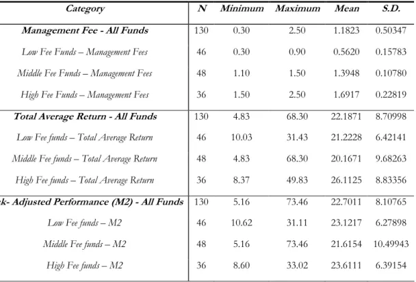
The table below gives an overlook of the descriptive statistics of the mutual funds used in this research. As mentioned previously the data consists of 130 Swedish based equity funds, dating back from 2003-2005, who invests on the global market.
The descriptive statistics concerning the management fee illustrates that the lowest fee charged by the mutual funds is 0.30 percent while the highest is 2.5 percent. The average management fee of all funds is 1.18 percent.
The total average returns illustrates that the average returns of the high fee funds (26.1 per-cent) exceeded the average returns of the low fee funds (21.2 perper-cent), and middle fee funds (20.2 percent). However, one can see that the average returns of the middle fee funds (20.2 percent) were lower than the low fee funds (21.2 percent). However, all the funds are satisfying since they all have higher returns than the risk-free interest rate which was 2.4 percent during this period of time (2003-2005).
The M2 calculations are also very interesting since the risk-adjusted returns of the low fee funds (23.1 percent) and the high fee funds (23.6 percent) was almost the same while the middle fee funds had the lowest returns (21.6 percent).
Table 6-1 – Descriptive statistics (2003-2005)
Category N Minimum Maximum Mean S.D.
Management Fee - All Funds 130 0.30 2.50 1.1823 0.50347
Low Fee Funds – Management Fees 46 0.30 0.90 0.5620 0.15783
Middle Fee Funds – Management Fees 48 1.10 1.50 1.3948 0.10780
High Fee Funds – Management Fees 36 1.50 2.50 1.6917 0.22819
Total Average Return - All Funds 130 4.83 68.30 22.1871 8.70998
Low Fee funds – Total Average Return 46 10.03 31.43 21.2228 6.42141
Middle Fee funds – Total Average Return 48 4.83 68.30 20.1671 9.68263
High Fee funds – Total Average Return 36 8.37 49.83 26.1125 8.83356
Risk- Adjusted Performance (M2) - All Funds 130 5.16 73.46 22.7011 8.10765
Low Fee funds – M2 46 10.62 31.11 23.1217 6.27898
Middle Fee funds – M2 48 5.16 73.46 21.6154 10.49943
High Fee funds – M2 36 8.60 33.02 23.6111 6.39154
6.2
Results
The results that were retrieved from a linear regression are presented below to show the reader what was retrieved from the regressions.
6.2.1 Regression 1 & 2
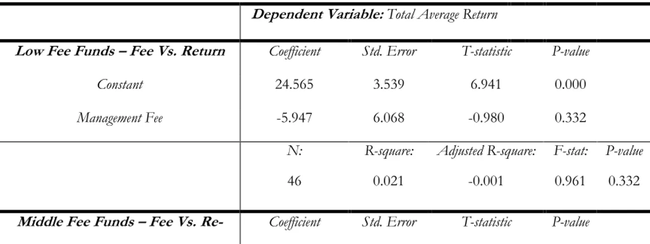
This regression tests if there is in fact a relation between the management fee of the funds and the total average returns.
Table 7-2 illustrates a linear regression analysis of all the available funds. The R-square can only explain 0.9 percent which is very low. This indicates that only 0.9 percent of the total average return can be determined by the management fee. Therefore the relation between the returns and the management fee is weak. It is also clear that the P-value exceeds the 5 percent significance level which indicates that it is insignificant.
Table 6-2 – Regression 1: Management fee Vs. Total average return (2003-2005) All Fee Funds – Fee
Vs. Return
Dependent Variable : Total Average Return
Coefficient Std. Error T-statistic P-value
Constant 20.293 1.955 10.378 0.000 Management Fee 1.602 1.523 1.052 0.295 N: 130 R-square: 0.009 Adjusted R-square: 0.001 F-stat: 1.107 P-value 0.295
Table 7-3 illustrates the results from regression 2. The data have been divided into three different categories to illustrate whether or not there is a higher significant value between the variables, and also this was done to demonstrate if low/middle/high fee charging mu-tual funds have a higher relation to the returns and the risk-adjusted returns of their respec-tive variables.
The low fee charging mutual funds have an R-square value equal to 2.1 percent which is higher than it was in table 7-2, however it is still very low. And the P-value was very high at 33.2 percent (> 5).
The middle fee charging funds had an R-square value of 13.4 percent which means that 13.4 percent of the total average return can be determined by the management fee, this is the highest value retrieved so far. The P-value is 1.1 percent which is lower than the 5 per-cent significance level and thus making it a significant value.
The high fee charging funds had the lowest R-square of the three categories (0.1 %) and the highest P-value (87.5 %) which is higher than the 5 percent significance level and thus making it an insignificant value.
Table 6-3 – Regression 2: Management fee Vs. Total average return (2003-2005) Dependent Variable: Total Average Return
Low Fee Funds – Fee Vs. Return Coefficient Std. Error T-statistic P-value
Constant 24.565 3.539 6.941 0.000 Management Fee -5.947 6.068 -0.980 0.332 N: 46 R-square: 0.021 Adjusted R-square: -0.001 F-stat: 0.961 P-value 0.332
turn Constant 65.948 17.244 3.824 0.000 Management Fee -32.823 12.327 -2.663 0.011 N: 48 R-square: 0.134 Adjusted R-square: -0.115 F-stat: 7.090 P-value 0.011
High Fee Funds – Fee Vs. Return Coefficient Std. Error T-statistic P-value
Constant 27.893 11.326 2.463 0.019 Management Fee -1.052 6.636 -0.159 0.875 N: 36 R-square: 0.001 Adjusted R-square: -0.029 F-stat: 0.025 P-value 0.875 6.2.2 Regression 3 & 4
This regression analysis will test if there is a relation between the fee of the funds and the risk-adjusted returns, using the M2 measurement. The results are presented in table 7-4. Table 7-4 shows that there is no relation between the management fee and the risk-adjusted returns at the 5 percent significance level. Looking at the R-square, the reader can clearly see that only 0.6 percent of the risk-adjusted performance can be explained by the fund fees, therefore the relation between the returns and the management fee is weak. The P-value which exceeds the 5 percent significance level (39.4 > 5), this clearly indicates that it is insignificant.
Table 6-4 – Regression 3: Management fee Vs. Risk-adjusted return (2003-2005) All Fee Funds – Fee
Vs. M2
Dependent Variable : M2
Coefficient Std. Error T-statistic P-value
Constant 24.138 1.823 13.242 0.000 Management Fee -1.215 1.419 -0.856 0.394 N: 130 R-square: 0.006 Adjusted R-square: -0.002 F-stat: 0.733 P-value 0.394
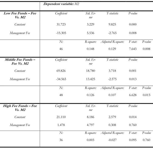
The results from the regressions in table 7-5, have again been separated into three different categories; low-, middle-, and high fee funds.
Looking at the low fee charging mutual funds where the risk-adjusted performance of the funds is situated against the fees, one can see that the findings illustrate some relation be-tween the two variables. This is illustrated when looking at the R-square which is almost 15 percent.
The findings of the “middle fee funds” also show a high R-square of 12.6 percent and a P-value of 1.3 percent, which is lower than the 5 percent significance level.
The high fee charging funds illustrates a low R-square of 0.3 percent and a high P-value of 76.0 percent which is higher than the 5 percent significance level and thus making it an in-significant value.
Table 6-5 – Regression 4: Management fee Vs. Risk-adjusted return (2003-2005) Dependent variable: M2
Low Fee Funds – Fee Vs. M2
Coefficient Std.
Er-ror T-statistic P-value
Constant 31.723 3.229 9.825 0.000 Management Fee -15.305 5.536 -2.765 0.008 N: 46 R-square: 0.148 Adjusted R-square: 0.129 F-stat: 7.643 P-value 0.008
Middle Fee Funds – Fee Vs. M2
Coefficient Std.
Er-ror T-statistic P-value
Constant 69.826 18.780 3.718 0.001 Management Fee -34.565 13.425 -2.575 0.013 N: 48 R-square: 0.126 Adjusted R-square: 0.107 F-stat: 6.628 P-value 0.013
High Fee Funds – Fee Vs. M2
Coefficient Std.
Er-ror T-statistic P-value
Constant 21.110 8.186 2.579 0.014 Management Fee 1.478 4.797 0.308 0.760 N: 36 R-square: 0.003 Adjusted R-square: -0.027 F-stat: 0.095 P-value 0.760
7
Discussions
This chapter will analyze the results retrieved from the regressions and connect them to previous researches in the same field. This is done to compare the results in this research to others in order to observe possible similarities and also to give the thoughts of the writer.
7.1
Regression 1 & 2
Looking at the descriptive statistics (table 7-1), one can see that there is a large difference in management fees between the different funds. Some funds demanded a management fee lower than 0.5 percent while others required a management fee higher than 2 percent. The
empirical results showed that there was not a significant relation between the management fees and the returns (un-adjusted and risk.-adjusted).
Table 7-2 and 7-3 illustrated the results from a linear regression which was conducted to assert whether or not there was a relationship between the management fee and the total average returns.
When reviewing all the funds that were used in this research in regression 7-2, the reader can observe that there were no significant relationship between the management fees and the total average returns. This can obviously only mean that the mutual funds available in this study do not have a relation to the management fees, and therefore the null-hypothesis is accepted. Carhart (1997) found in a similar study that funds with higher expense levels performed worse than the low-expense funds. This is of course a failure from the fund companies because if they charge the investors a higher management fee, they should gen-erate higher returns. Otherwise the fund companies should either lower their fees or make a higher effort in managing the fund in order to please the expectations of an investor. Table 7-3 displays all the funds categorized according to their fees; low-, middle-, and high fee funds. This division was completed to analyze the connection between the management fee in the different categories and their respective total average returns. The findings of the low fee funds illustrate no relation between the fees and the total average returns in that category which again means that the null-hypothesis is accepted.
The middle fee funds in table 7-3 showed a higher R-square value and were significant at the 95 percent confidence level, which means that there was a connection between the management fees and the total average returns and therefore the null-hypothesis was re-jected. This means that there is some justification to the higher fees in the middle fee cate-gory since higher returns were generated. However, these results could be somewhat biased since the difference between the average returns between the mutual funds in this category was the largest. The findings in the descriptive statistics (table 7-1) illustrates that the high-est total average returns in the middle fee category was 68.3 percent which was also the highest in this study, while the lowest was 4.83 percent which also was the lowest in this study. The middle fee category also illustrated the highest standard deviation of all the cate-gories which shows that the returns fluctuate heavily in this category.
The findings of the high fee charging funds in table 7-3 illustrates a very low R-square value and an insignificant value at the 95 percent confidence level, which is why the null-hypothesis is rejected. The findings show that the high management fees are not justified by achieving higher returns. The fund managers should either work harder to generate higher returns or lower their fee.
7.2
Regression 3 & 4
Regression 3 & 4 examined whether or not there exist any relationship between the mutual fund management fee charged by the fund companies and their respective risk-adjusted performance, which was calculated by using the M2 measurement.
The findings in table 7-4, which illustrates a linear regression of all the mutual funds used in this research, clearly this shows that there was no sign of a relationship between the two variables (management fee and the risk-adjusted returns). This could only mean that it does not matter whether a fund charges a high fee or a low fee, since this will not affect the risk-adjusted performance and therefore the null-hypothesis is accepted. This contradicts the results of Dellva and Olson (1998), who stated in their study that one should most likely
expect a lower or even a negative risk-adjusted performance if a mutual fund charges zero in management fee
Table 7-5 illustrates a dividedness of the mutual funds. All the categories of the different fees are tested against their respective risk-adjusted performance in a linear regression. The low fee charging mutual funds illustrates the highest R-square value in this research and a significant value at the 95 percent confidence level. These findings illustrate the most sig-nificant values in this research and therefore the null-hypothesis was rejected. One can see that there is a relationship between the low fee charging mutual funds and the risk-adjusted returns. The results from the descriptive statistics also reveals that the standard deviation of the risk-adjusted returns of the low fee charging mutual funds was the lowest and thus meaning that there were low fluctuations. A research that was presented by Harris in 1997 showed that low fee charging mutual funds outperformed the high fee charging mutual funds, which is in line with what the findings of the low fee charging funds illustrated. The middle fee charging mutual funds also showed a high P-value, compared to the results from regression 7-4, and also a significant value at the 95 percent confidence level and therefore is the reason to why the null-hypothesis is rejected. One can see that the fees in this category are somewhat justified by higher returns. Once again the standard deviation, which is found in table 7.1, is the highest in the risk-adjusted performance category with approximately 10.5 percent which illustrates that there are high fluctuations in this cate-gory.
Once again the high fee charging mutual funds disappoints. These funds are charging high fees without achieving high risk-adjusted returns and therefore are the reason to why the null-hypothesis is accepted. This is of course a failure from the mutual fund companies. The lower risk-adjusted returns in this category could in fact be a result of the higher fees. This is something that the mutual fund companies needs to take a look at and also analyze the situation to achieve a good outcome for the investors, for themselves and for their funds.
8
Conclusion
The purpose of this thesis was to evaluate whether or not there is a relationship between low fee, middle fee, and high fee charging Swedish Equity funds and their respective per-formance, unadjusted and risk-adjusted returns.
The conclusion is that there was no significant relationship between low fee, middle fee, and high fee charging Equity funds and their respective performance, unadjusted and risk-adjusted returns.
It was found that low fee and middle fee charging mutual funds often had a higher degree of connection (not necessarily high) with their respective total average returns and the risk-adjusted returns, while the high fee charging funds did not show any signs of some kind of relationships with its total average returns and risk-adjusted returns. This is in accordance with the findings of Blake, Elton and Gruber (1993) who believed that, after performing a regression analysis of expense ratios against the risk-adjusted performance, investors who do not possess the knowledge of evaluating mutual funds should invest in low expense funds.
To summarize, one can say that a mutual fund that charges a high management fee does not necessarily generate higher returns. An investor should always thoroughly evaluate the
mutual funds, securities etc. that he/she intend to invest in before making a mistake by choosing the wrong one, that will not fulfil his/her expectations. When buying a product or a service, one should always focus on the quality rather than the price.
8.1
Further Studies
Some interesting questions have been brought up during this study. Some of them are pre-sented below to show other people what kind of studies they could conduct to enrich the mutual funds research.
An interesting study would be to test whether or not risk has any effects on the mutual fund fees. Do mutual funds that contain higher risk also contain higher or lower manage-ment fees?
Another interesting study would be to test how the macroeconomic environment affects the returns of a specific category of mutual funds. One could for instance test if the dollar fluctuation affects the mutual funds etc.
References
Blake, C. R. Elton, E. J. Gruber, M. J. (1993) The performance of bond mutual funds. Journal of Business. Vol. 66
Blake, C. R. Morey, M. (2000). Morningstar Ratings and Mutual Fund Performance. Journal of Financial and Quantitative Analysis.
Carhart, M. (1997). On persistence in mutual fund performance. Journal of Finance. Dahlquist, Magnus. Engström, Stefan. Söderlind, Paul. (2000). Performance and character-istics of Swedish Mutual Funds. Journal of Financial and Quantitative Analysis. Vol. 35 Dellva, Willfred L. Olson, Gerard T. (1998). The relationship between Mutual fund fees and expenses and their effects on performance. The Financial Review.
Dhankar, Raj S. Singh, Rohini. (2005). Arbitrage pricing theory and the Capital Asset Pric-ing Model-Evidence from the Indian stock market. Journal of financial management & analysis. Vol. 18.
Fabozzi, Frank. Modigliani, Franco. Ferri, Michael, G. (1994). Foundations of financial markets and institutions. New Jersey; Prentice-Hall, Inc.
Fama, Eugene. French, Kenneth. (2003). The CAPM: Theory and evidence. Center for re-search in security prices, University of Chicago. No. 550.
Frino, Alex. Gallagher, David R. (2002). Is index performance achievable? An analysis of the Australian Equity index funds.
Grinblatt, M. Titman, S. (1989). Mutual fund performance: An analysis of quarterly portfo-lio holdings. Journal of Business, Vol. 62.
Grinblatt, M. Titman, S. (1994). A study of monthly mutual fund returns and performance evaluation techniques. Journal of Financial and Quantitative Analysis. Vol. 29.
Guo, Hui. (2004). A Rational pricing explanation for the failure of the CAPM. Federal re-serve bank of Saint Louis. Journal of financial management & analysis. Vol. 86.
Harris, J. (1997). Big fees, small results. Canadian Business. Vol. 70.
Ianthe, Jeanne D. (2005). Sharpe Point: Risk Gauge Is Misused. New York. Wall Street Journal.
Jensen, M. C. (1968). The performance of mutual funds in the period 1945-1965. Journal of Finance. Vol. 23.
Lawton-Browne, Carola (2001). An alternative calculation of tracking error. Journal of As-set Management. Vol. 2
Lind, Douglas A. Marchal, William G. Mason, Robert D. (2002). Statistical techniques in business & economics. Boston. McGraw-Hill Irwin.
Lintner, John. (1965). Security prices, risk and maximal gains from diversification. Journal of Finance.
Modigliani, Franco. Modigliani, Leah. (1997). Risk-Adjusted Performance. Journal of Port-folio Management.
Nilsson, Pia. (2004). Fondboken. Stockholm, Sellin & partner: Fondbolagens förening. Padgette, Robert L. (1995). Performance reporting: The basics and beyond, Part II. Journal of financial planning. Vol. 8.
Sharpe, William (1964), Capital Asset Prices: A Theory of Market Equilibrium under Con-ditions of Risk. The Journal of Finance.
Sharpe, William (1966), Mutual Fund Performance. Journal of Business. Vol. 39.
Simons, Katerina. (1998). Risk-adjusted performance of mutual funds. New England Eco-nomic Review.
The capital asset pricing model. (1998). New England Economic Review.
Treynor Jack. (1961). Toward a theory of market value of risky assets. Unpublished manu-script.
Treynor Jack. (1965). How to Rate Management of Investment Funds. Harvard Business Review. Vol. 44.
Wermers, R. & Moskowitz, T.J. (2000). Mutual Fund Performance. Journal of Finance.
Internet sources:
Morningstar - www.morningstar.se, www.morningstar.com Finansinspektionen - www.fi..se
Aktiespararna - www.aktiespararna.se Riksgäldskontoret - www.rgk.se
Fondbolagens förening - www.fondbolagen.se