Sensitivity of irrigation water supply to climate change in the Great Plains region of Colorado

Full text

(1)Hydrology Days 2005. Sensitivity of Irrigation Water Supply to Climate Change in the Great Plains Region of Colorado. Elgaali Elgaali1 Ph.D., Research Fellow, Integrated Decision Support Group, Civil Engineering Department, Colorado State University, Fort Collins. Luis A. Garcia Director Integrated Decision Support Group and Associate Professor, Civil Engineering Department, Colorado State University, Fort Collins. Abstract: Increasing amounts of atmospheric carbon dioxide are expected to raise atmospheric temperature and lead to significant changes in global climate during this century. Global warming may have tremendous consequences for irrigated agriculture around the world. This paper investigates the possible effects of such climatic changes on water resources available for agriculture in the Arkansas River Basin in Colorado. The potential impacts of climate change on this region include changes in winter snowfall and snow melt, seasonal rainfall amounts and intensities and winter and summer time average temperatures. For this study, a framework was developed to quantify the effects of these seasonal impacts on the availability of irrigation water. Monthly surface water supplies, consumptive use, and water balances were estimated using neural networks, consumptive use, and water balance models respectively. Two transient climate scenarios extracted at high resolution from two General Circulation Models (GCMs); the HAD (Hadley Center) and the CCC (Canadian Center) were used. The climate scenarios were run assuming a 1% annual increase in CO2 concentrations. The methodology and results described in this study are contributing to the national analysis of impacts of climate change on the water sector.The frame work developed as part of this research will help a region plan for changes in water supply and demand and will give decision-makers a tool for evaluating the impacts of climate change. Furthermore, the data driven nature of the frame work makes it flexible so that it can be applied to different areas.. 1.. Introduction. In many areas of the world, agricultural production is threatened by water supply shortages. Currently, about 17% of the world’s cropland is under irrigation (Rosenzweig and Hillel 1998). In the United States, irrigation represents about 81% of the total water demand and consumes 41% of the water supply (Solley et al. 1997). In the Great Plains of the United States, surface water supplies have been declining since 1980 forcing 12% of the 1. Integrated Decision Support Group Civil Engineering Department Colorado State University Fort Collins, CO 80523-1372 Tel: (970) 491-7620 e-mail: gaali@engr.colostate.edu. ©Hydrology Days. 258.

(2) Sensitivity of Irrigation Water Supply to Climate Change in the Great Plains of Colorado. cropland in the region to be retired from irrigation (Dugan et al., 1994). Currently, changes in water utilization are making the competition for water between agriculture and other uses (e.g. urban development) more intense (Ojima et al., 1999). There is mounting evidence that increasing amounts of carbon dioxide (CO2) may lead to significant changes in global climate during this century (IPCC 2001). Increasing amounts of CO2 and other greenhouse gases will raise global temperatures causing what is known as global warming. Global warming, if it occurs as projected, might have important impacts on water resources and agriculture. Climate change is expected to further stress water resources. It might widen the gap between the demand for, and supply of, water for irrigation. The changing climate and elevated atmospheric CO2 are expected to influence irrigation by changing evapotranspiration, precipitation, and available water supplies. The combined effect of these changes would impact the supply and the demand of water. Generally, under warmer conditions the water supply is expected to decrease as demand increases due to rising rates of evaporation and transpiration (Peterson and Keller 1990). Also, in an environment of increased temperature and evaporation, the lack of available water can further stress soil moisture. Stress in soil moisture can greatly reduce agricultural yield (Rosenzweig and Hillel, 1993; Rosenzweig and Hillel, 1998; Ojima et al., 1999). On the other hand, the physiological effects of high levels of CO2 on plants, may affect irrigation demand. Generally, high levels of CO2 enhance stomata closure (the pores in the plant leaf through which water vapor and CO2 are exchanged with the atmosphere) and increase the plant foliage (increase plant leaf area). Increase in stomata closure reduces the transpiration in the plant. Meanwhile, an increase in leaf area means a greater number of stomata and hence an increase in transpiration. Naturally, climate-water-agriculture interactions are of concern not only to the scientific community but to policy makers as well. Proper understanding of these interactions under climate change might help to mitigate the adverse impacts of global warming while selectively reinforcing the positive impacts. Indeed, potential climate change impacts have been assessed for decades. As our understanding about the extent and magnitude of climate change has improved, the need for accurate and detailed predictions of what might occur in the future has become increasingly urgent. A number of studies have used historical analogues and projected climate scenarios to assess the risk to agriculture from climate change (Rosenberg et al., 1990; Peterson and Keller, 1990; Allen et al., 1991; Rosenberg et al., 1993; Peart et al., 1995). Recent works by Eheart and Tornil, 1999; Ojima et al., 1999; and Jones, 2000 represent a further step in modeling climate change impacts.The previous studies have used a variety of projected climate change scenarios to estimate a range of potential impacts. Different climate, ecosystem, and water balance models have been developed to estimate the parameters of the soil-vegetation-atmosphere interactions. However, many of these models are of limited use because they lack precision due to their coarse. 259.

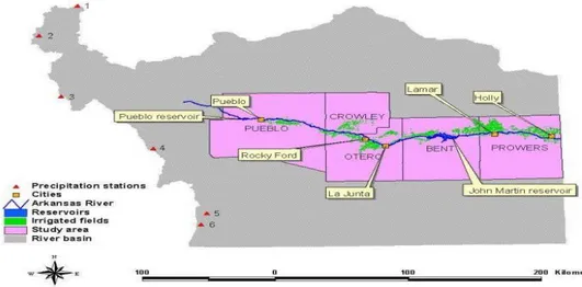
(3) Elgaali and García. spatial resolution. In addition, the precipitation and hydrological cycles that are especially critical for agriculture are often poorly simulated (Rosenzweig and Hillel, 1998). Furthermore, the real impact of climate change on irrigation can best be evaluated in presence of the two irrigation balance components (supply/demand).models must be available for evaluation of large-scale planning targets in view of detailed design and management issues that arise at smaller scales (Ojima et al., 1999). The research described here provides a modeling methodology for linking agriculture water potentials to climate change on a scale useful to addressing the distributed nature of the problem. The main goal of this research is to improve the estimates of potential impacts of regional climate change on irrigation water by improving key features of previous research. The improvements include: resolution of climate scenarios (higher), spatial representation of the problem, scale of analysis (monthly and seasonal) of responses and sensitivities to climate changes, and use of multiple crops.. 2.. Description of Study Area. This study focuses on the Arkansas River Basin in Colorado. Bounded on the west by the Rocky Mountains, on the east by Kansas, and by New Mexico and Oklahoma on the south (Figure 1), the area covers approximately 72,742 km2 (28,415 square miles). The basin encompasses about 27 percent of the state of Colorado. The headwaters of the Arkansas River are located near Leadville, at an elevation of over 3,050 m (10,000 feet) above mean sea level. From there, the Arkansas River’s elevation drops rapidly until it emerges from the mountains near Pueblo. The river then runs in an easterly direction until it reaches the Colorado-Kansas border near Holly, Colorado at an elevation of about 1,036 m (3,400 feet).. Figure 1. Features of the study area in the Arkansas River Basin, Colorado. In the Arkansas River Basin, temperature and precipitation vary widely in response to topographic differences. Average annual temperatures ranges 260.

(4) Sensitivity of Irrigation Water Supply to Climate Change in the Great Plains of Colorado. from 2o C at Leadville in the mountains to 12° C at Lamar in the lower valley. Seasonal variations in temperature are very large. The average frost free season (32 oF threshold) varies from 85 days at Leadville to 167 days at Canon City. Precipitation is distributed unevenly throughout the year. Precipitation ranges from 9 to 12 inches per year in the middle and eastern parts of the region, 16 to 20 inches in the western part, and as much as 45 inches in the highest mountain ranges. At high elevations, much of the precipitation occurs as snow. Runoff from this snowfall constitutes the principal water supply for the region. In general, more than 60 percent of the average annual runoff occurs between April and July, with 20 percent occurring between August and October. Lakes and reservoirs in the basin serve to store natural runoff, which generally peaks during May or early June, for use when needed. Peak demand for water usually occurs in July and August. Trans-basin diversions are also a significant addition to the basin water supply. There is an extensive system of canals, tunnels, and reservoirs for collecting and transporting water from the western side of the Continental Divide to the Arkansas Basin. Water is applied to crops and pasture in the basin through a huge system of ditches and canals. Twenty of the major canals are included in this study. Table 1 shows the total diversions for those canals being studied. Table 1. Total diversions for canals studied Ditch Bessemer Booth Excelsior Collier Colorado RF Highline Oxford Otero Catlin Holbrook Rocky Ford Ft Lyon Las Animas Fort Bent Keese Amity Lamar Manvel Hyde XY Graham Buffalo Total. Hectares Served 7028 189 875 203 9279 8020 1910 1159 6943 5286 2184 35602 2637 1768 754 15252 3180 499 1764 1984 106515. Diversions (ha-m) 7760 497 293 86 10680 10284 3067 838 10990 5274 5381 29900 3898 2067 660 9890 5086 284 1107 2437 7760. In general, the average amount of water diverted to these systems is 0.43 hectare-meter for 106,515 hectares (3.5 acre feet for 263,000 acre) served (20. 261.

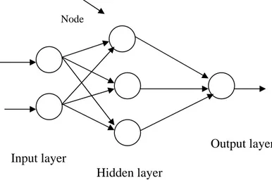
(5) Elgaali and García. canals). The surface diversion data was summarized from records of the Colorado State Engineer’s Office in Denver.. 3.. Methods. 3.1 Model description 3.1.1 Water Supply Model Water supply was modeled using an Artificial Neural Network (ANN) model. ANNs are able to learn, estimate and generalize a relationship between inputs and outputs of the same pattern in a system. ANNs can be trained to map any non-linear complex relation. During the training process, the network is presented with a set of inputs and a set of outputs and is trained to use the inputs to produce the most accurate estimates for the outputs. Once properly trained, the network provides a data driven model, which is capable of giving reasonable answers when presented with input vectors that have never been encountered during the training process. The key to successfully training an ANN is choosing the right network structure and training algorithm. Network structure (architecture) includes the number of interconnected layers in the network and the number of neurons in each layer. The dimension of the input and output data set presented to the network for training dictates the number of neurons in each related layer (input and output) while trial and error is the usual method used for determining the number of hidden layers and number of neurons and activation (transfer) functions in each layer. In this study a feedforward 5-5-1 neural network (ANN) like the one shown in Figure 2 was used to map the relation between the water diverted for irrigation in the region (output) and the streamflow/precipitation (input). A feedforward ANN having a finite number of neurons in the hidden layer was proved to be a universal function that can approximate any multivariate function (Hsu et al. 1995). Node. Output layer Input layer Hidden layer Figure 2. Feedforward 2-3-1 neural network. Extensive correlation analysis and numerous data sets were used to select predictors that maximize the potential of the ANN model to simulate the water. 262.

(6) Sensitivity of Irrigation Water Supply to Climate Change in the Great Plains of Colorado. diversions. Three predictors: Qr (t), PPTm, and PPTb were used to predict the water diversions D; Qr is streamflow, PPTm is precipitation in the mountains, and PPTb is precipitation in the river basin area. The diversion D at time (t) is treated as a function of Qr, PPTm and PPTb at time (t) and (t-1) as follows: D (t) = f (Qr(t), PPTm(t), PPTm(t-1), PPTb(t), PPTb(t-1)) (1) 3.1.2 Water Demand model The model IDSCU that was used to predict irrigation water demand was developed by the Integrated Decision Support group (IDS), Civil engineering department, Colorado State University (http://www.ids.colostate.edu). The model incorporates monthly and daily methods to estimate evapotranspiration (ET). The model estimates the ET from weather data files and applies crop and area information to determine the consumptive use (CU). The model applies the available water supply and weather data to determine the water use of various crops during the growing season. Surface water supplies can be specified. If there is additional CU beyond the surface supplies; wells can be assumed to supply the additional CU. Weights can be assigned to weather stations, reflecting their relative influence. The computation of ET includes an option for calculating a soil moisture budget. The methods in the model can be used to develop scenarios of CU from scenarios of climate and plant data. This makes IDSCU capable of estimating as well as evaluating the impacts of climate change on irrigation water demand. IDSCU is capable of accommodating the variability of crops and soils within the modeling area. The model is also flexible enough to be used to project the combined impacts on irrigation demand from the global warming and plant physiological responses to elevated atmospheric CO2. ET was estimated on a daily time step using Penman-Monteith combination method (ASCE, 1990). Maximum and minimum daily temperature, solar radiation, relative humidity, wind speed, and monthly precipitation were inputs to the model. IDSCU was run on 5 representative sub-areas and different crop systems to reproduce the spatial complexity of irrigation water demand in the region. 3.2 Models Testing and Validation Both models were validated against measured data for the area of study. Ninety years of data records (1911 – 2000) were used in calibrating (training) and validating the neural network model. The data was portioned into three parts: 1) 1911-1960 for training, 2) 1961-1975 for validation, and 3) 19762000 for testing. Testing is a post-analysis process to check the performance of the network, in which a regression analysis is made between the network model output (simulated) and the target (measured). The relation between the two outputs (simulated/measured) is indicated by the best line fit and the correlation coefficient (R). If the slope of the best line fit and the correlation coefficient approach the value 1, this is an indication of the ability of the network to map the target output very well. The performance statistics. 263.

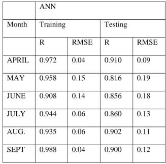
(7) Elgaali and García. described in Table 2 were used to summarize the relationships between the output of the network and the target values being modeled. Obviously, the ANN model explained an average of 85% of the variance of the measured monthly data for the years 1976-2000. Table 2. Summary of ANN model validation and testing ANN Month. Training. Testing. R. RMSE. R. RMSE. APRIL. 0.972. 0.04. 0.910. 0.09. MAY. 0.958. 0.15. 0.816. 0.19. JUNE. 0.908. 0.14. 0.856. 0.18. JULY. 0.944. 0.06. 0.860. 0.13. AUG.. 0.935. 0.06. 0.902. 0.11. SEPT. 0.988. 0.04. 0.900. 0.12. The Penman-Montieth method that was used to estimate ET is already calibrated under different climatic conditions including the ones that prevail in the study area. Currently several scientific agencies (e.g. COAGMET) use this method to estimate the ET in the study area. However, to evaluate the accuracy of the ET method for the purpose of this study, the reference ET (alfalfa) values computed by the water demand model were validated against measured and computed (COAGMET) data for the same period of time (Table 3). The measured data is part of a project to determine the salinity levels and sources in lower Arkansas River Basin. In this project (www.ext.colostate.edu) atmometers were used to measure ET values in fields of alfalfa and other crops. The Penman-Montieth model reliably produced results in a good agreement with the results of the other sources. Table 3. Comparison of ET values Source. ET mm (inches). COAGMET. 1,165 (45.89). Model (P-M). 1,175 (46.25). Atmometers. 1,135 (44.68). 264.

(8) Sensitivity of Irrigation Water Supply to Climate Change in the Great Plains of Colorado. 3.3 Climate Data The Vegetation-Ecosystem Modeling and Analysis Project (VEMAP) (Kittel et al., 1995) provided climate data used in this study. The VEMAP involves the development of climate data sets for the continental United States. The climate data includes historical data from 1895-1993, and projections from two GCM’s based transient scenarios for 1994-2099. The two GCM’s scenarios are the transient HAD which was developed by the Hadley Center for Climate Prediction and Research, United Kingdom and the transient CCC, which was developed by the Canadian Center for Climate Prediction and Analysis. The historical time series were derived from: a) variable length data records from 1895-1990 (1200 stations) and b) short data records from 19511990 (6000-8000 stations). The two GCM’s models generated future climate data (projections) using physics laws, assuming 1% annual increase in CO2 concentrations. The National Center for Atmospheric Research (NCAR) as part of VEMAP processed, spatially interpolated (downscaled), and topographically adjusted the historical and the projected climate data to the 0.5o lat/long VEMAP grid (for the VEMAP the conterminous US was divided into 0.5oX0.5o grid cells in order to simulate small-scale influences such as local topography and ecosystems on climate) (Kittel et al., 1997). The downscaling process accounted for the effects of local topography on climate parameters. Therefore, this high resolution is partially controlled by the local-scale changes.. 4.. Results and Discussion. In general, the water resources available for use in a region are determined by the amount of water available (supply) and the amount of water needed (demand). In this region the water supplies determine the amount of water available for use (demand). Climate change is expected to affect both water supply (WS) and water demand (IWR) for irrigation therefore, it is necessary to examine the potential changes in the balance between demand and supply under climate change. This section of the paper explores the status of the balance between demand and supply under two scenarios of climate change. The effects of climate change were evaluated using water balance sheets. To show the extent and magnitude of climate change impacts, the sensitivity of the irrigation water balance under climate change was compared to its behavior under no climate change conditions (baseline). First, a baseline irrigation water balance was established using historical records of water supply and demand. Table 4 shows the irrigation water balance of the historical averages for the region. The numbers and percentages presented (Table 4) show that under the baseline (no climate change) water supplies were already under stress during the summer months. During the summer time of the growing season the region experiences a shortage in water supplies, which can reach up to 28% (on average) of water demand. To fill the gap between demand and surface. 265.

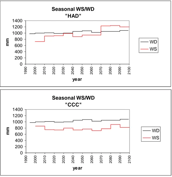
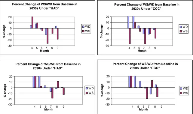
(9) Elgaali and García. supply, groundwater supplies have been used conjunctively with surface supplies. Groundwater has been pumped to augment 5-10 % of the deficits presented in Table 4. The values show that in June the shortage was up to 13% (28mm) of the water demand, while the percentage varies among the other summer months from 29% (70mm) in July, 41% (94mm) in August, 31% (37mm) in September, and 13% (117mm) during the whole season. Table 4. Historical water demand – water supply balance Water demand. Water supply. Difference. mm. mm. mm. Apr.. 9. 90. 81. surplus. 900. May. 109. 140. 31. surplus. 28. June. 216. 188. 28. deficit. 13. July. 244. 173. 70. deficit. 29. Aug.. 230. 136. 94. deficit. 41. Sept.. 118. 81. 37. deficit. 31. Season. 926. 809. 117. deficit. 13. Difference type. Difference. %. Climate change further stressed surface water supplies and increased water demand especially during the summer time, outweighing the balance of irrigation water. However, there are ways to mitigate the impacts (water shortage) of these effects on agricultural water systems one of which is the use of groundwater supplies. As mentioned in the previous paragraph groundwater is used to augment only 5-10% of the historical shortage in surface water supplies. For the purpose of this study, any difference between demand and supply in the future (under climate change) greater than 5-10% is considered a deficit, assuming that we have enough groundwater stored to provide the same current amounts of groundwater supplies (5-10%). Figure 3 compares projections of seasonal water supply and demand under two climate scenarios (HAD/CCC). Obviously, under the CCC scenario water supplies in the region is expected to be too short to satisfy the demand and the gap between WS/WD is wider than that under the HAD scenario. The figure also show that the gap between WS/WD under the HAD scenario is variable and is expected to be narrowed and vanish by the end of decade 2060s and the region is expected to have enough water supplies. Figure 4 compares projections in percent change from baseline of monthly WS/WD in decades 2030s and 2090s (mid and the end of 21st century). The figure shows the vigorous variation in irrigation balance within the months of the growing. 266.

(10) Sensitivity of Irrigation Water Supply to Climate Change in the Great Plains of Colorado. season. eason. As shown in the figure most of the shortages are expected during the summer with large amount of water supplies are expected during the spring.. 1400 1200 1000 800 600 400 200 0. WD. 2100. 2090. 2080. 2070. 2060. 2050. 2040. 2030. 2020. 2010. 2000. WS. 1990. mm. Seasonal WS/WD "HAD". year. 1400 1200 1000 800 600 400 200 0. WD. year. Figure 3. Comparison of seasonal water supply and demand. 267. 2100. 2090. 2080. 2070. 2060. 2050. 2040. 2030. 2020. 2010. 2000. WS. 1990. mm. Seasonal WS/WD "CCC".

(11) Elgaali and García. Percent Change of WS/WD from Baseline in 2030s Under "HAD". Percent Change of WS/WD from Baseline in 2030s Under "CCC" 20. 20. 10 WD. 0. WS -10. % change. % change. 10. WS -10 -20. -20 -30. 4. 5. 6 7 8 Month. -30. 9. 5. 6 7 8 Month. 9. 20. 20. 10. 0. WD. -10. WS. % change. 10 % change. 4. Percent Change of WS/WD from Baseline in 2090s Under "CCC". Percent Change of WS/WD from Baseline in 2090s Under "HAD". 0. WD. -10. WS. -20. -20 -30. WD. 0. 4. 5. 6 7 8 Month. 9. -30. 4. 5. 6 7 Month. Figure 4. Percent change in monthly water supply and demand. 268. 8. 9.

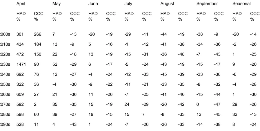
(12) Sensitivity of Irrigation Water Supply to Climate Change in the Great Plains of Colorado. Table 5 shows the difference (in percentage) between demand and supply under the two scenarios of climate change. The results show that under the CCC scenario the region is expected to experience a shortage in water supply for long periods of time which extend from the 2010s to the 2090s. Shortages are expected for the whole season and for each month in the season except for April. The maximum shortage for the whole season (30%) is expected during the decade of the 2060s. While no shortage is expected during the decade of the 2080s, the shortage during the decade of the 2090s is expected to be double the current shortage in surface water supply. The shortage during the summer time is greater than that during the spring. The results show that, under the HAD scenario the region is expected to have shortage in water supplies during the summer time (August) of the growing season, while the whole growing season is shown to have no shortage in water supply. This due to the fact that the high water supplies projected for the spring are high enough to offset the shortage expected during the summer assuming that there is enough storage infrastructures to store the large amount of water supplies expected during the spring so that they can be used during the summer time.. 5.. Summary. The real impact of climate change in either water supply or water demand can best be evaluated in conjunction with the other. The balance of water supply and demand for irrigation could be affected the differences in temperature and precipitation changes projected by the two scenarios. The results presented show that the region already experiences shortages in surface water supply and a relatively small percentage (5-10%) of these are augmented by groundwater. Under the CCC scenario the water balance deteriorates in the region because water supplies for the whole season and each month in the season (except for April) are expected to be short to satisfy the demand. Under the HAD scenario which is wet and less warm than the CCC scenario the changes in the balance between supply and demand range from no significant changes to improvement due to increase in water supply over demand. The high projections of additional water supply during the spring are expected to offset the decreases projected in water supply during summer specifically in August. Therefore, the balance in the growing season under the HAD scenario is projected to improve. As discussed in a previous section (section 6.2) this last result is uncertain in the absence of other factors such as enough water storage infrastructures to store the additional water projected during the spring and use it to offset the decrease of water during the summer. In general, under the HAD scenario the climate effects on the balance of supply and demand for irrigation would be more favorable in the last three decade of this century (2070-2090) while the water balance derived from the CCC projections deteriorates all the time.. 269.

(13) Elgaali and García. Table 5. Water balance under two scenarios of climate change (HAD and CCC) presented in percentages April. May. June. July. August. September. Seasonal. HAD %. CCC %. HAD %. CCC %. HAD %. CCC %. HAD %. CCC %. HAD %. CCC %. HAD %. CCC %. HAD %. CCC %. 2000s. 301. 266. 7. -13. -20. -19. -29. -11. -44. -19. -38. -9. -20. -14. 2010s. 434. 184. 13. -9. 5. -16. -1. -12. -41. -38. -34. -36. -2. -26. 2020s. 472. 150. 22. -18. 13. -19. -15. -31. -36. -48. -7. -43. 1. -25. 2030s. 1471. 90. 52. -29. 6. -17. -5. -24. -43. -19. -15. -17. 9. -20. 2040s. 692. 76. 12. -27. -4. -24. -12. -33. -45. -39. -33. -38. -6. -29. 2050s. 322. 36. -4. -30. -9. -22. -11. -21. -33. -35. -8. -32. -4. -28. 2060s. 609. 27. 21. -36. 11. -26. -7. -25. -41. -46. -15. -44. 1. -30. 2070s. 592. 2. 35. -35. 15. -19. 24. -29. -20. -42. 0. -47. 29. -26. 2080s. 598. 60. 39. -27. 19. -15. 15. 7. -8. -33. 12. -45. 32. -13. 2090s. 528. 11. 4. -43. 1. -24. -7. -26. -36. -33. -14. -38. 8. -24. 270.

(14) Sensitivity of Irrigation Water Supply to Climate Change in the Great Plains of Colorado. References Allen, R. G., F. N. Gichuki, and C. Rosenzweig. 1991. “CO2-induced climatic changes and irrigation requirements. Journal of Water Resources Planning and Management 117(2): 157-178. American Society of Civil Engineers (ACSE) Manual No. 70, 1990. Evapotranspiration and Irrigation Water Requirements. Colorado Water Conservation Board (CWCB) and USDA, 1981. Arkansas River Basin Report. Dugan, J. T., T. McGrath and R. B. Zelt. 1994. Water-Level Changes in the High Plains Aquifer-Predevelopment to 1992. U.S. Geological Survey. WaterResources Investigations Report 94-4027. Lincoln, NE. Frederick, K. D. 1997. Adapting to climate impacts on the supply and demand for water. Climatic Change 37(1): 141-156. Hsieh, W. W., and B. Tang, 1998. Applying neural network models to prediction and data analysis in meteorology and oceanography. Bulletin of the American Meteorological Society 79(9): 1855-1870. Hsu, K., H. V. Gupta, and S. Sorooshian, 1995. Artificial neural network modeling of the rainfall-runoff process. Water Resources Research 31(10): 22517-2530. IDS. (http://www.ids.colostate.edu) IPCC, Climate Change 2001: the scientific basis- summary for policy makers and technical summary for the working group 1 report. Cambridge University Press, UK, 2001. Jones, R. N., 2000. Analyzing the risk of climate change using an irrigation demand model. Climate Research 14:89-100. Kittel, T.G.F., N.A. Rosenbloom, T.H. Painter, D.S. Schimel, and VEMAP Modeling Participants (1995). The VEMAP integrated database for modeling United States ecosystem/vegetation sensitivity to climate change. J. Biogeog. 22:857-862. Kittel, T.G.F., J.A. Royle, C. Daly, N.A. Rosenbloom, W.P. Gibson, H.H. Fisher, D.S. Schimel, L.M. Berliner, and VEMAP2 Participants. (1997) A gridded historical (1895-1993) bioclimate dataset for the conterminous United States. In: Proceedings of the 10th Conference on Applied Climatology, 20-24 October 1997, Reno, NV. American Meteorological Society, Boston. Leavesley, G. H., 1994. Modeling the Effects of Climate Change on Water Resources- A Review. Climatic Change 28:159-177. Lane, M. E. P. H. Kirshen, and R. M. Vogel, 1999. Indicators of impacts of global climate change on US water Resources. Journal of Water Resources Planning and Management-ASCE 125(4): 194-204. McFarlane, N. A. G. J. Boer, J. P. Blanchet, and M. Lazare, 1992. The Canadian Climate Centre Second-Generation General Circulation Model and Its Equilibrium Climate. Journal of Climate 5: 1013-1044. Natural Resources Conservation Service (NRCS) - National Water and Climate Center (NWCC)-USDA 2003. Ojima, D., L. Garcia, E. Elgaali, K. Miller, T. G. F. Kittel, and J. Lackett, 1999. Potential Climate Change Impacts on Water Resources in the Great Plains. Journal of the American Water Resources Association 35(6): 1443-1454. Peart, R. M., R. B. Curry, C. Rosenzweig, J. W. Jones, K. J. Boote, and L. H. Allen, Jr, 1995. Energy and irrigation in south eastern U.S. agriculture under climate change. Journal of Biogeography 22: 635-642. Peterson, D. F. and A. A. Keller. 1990. Irrigation. In P. E. Waggoner (ed.). Climate Change and Water Resources. Wiley. New York. pp 269-306..

(15) Elgaali and García. Rosenberg, N. J., B. A. Kimball, P. Martin, and C. F. Cooper. 1990. From climate and CO2 enrichment to evapotranspiration. In P. E. Waggoner (ed.). Climate Change and Water Resources. Wiley. New York. PP 151-175. Rosenberg, N. J., P. R. Crosson, K. D. Frederick, W. E. Easterling, III, M. S. McKenney, M. D. Bowes, R. A. Sedjo, J. Darmstadter, L. A. Katz, and K. M. Lemon 1993. The MINK Methodology: Backgound and Baseline. Climatic Change 24: 7-22. Rosenzweig, C. and D. Hillel. 1993. The dust bowel of the 1930s: Analog of greenhouse effect in the Great Plains? Journal of Environmental Quality 22(1): 922. Rosenzweig, C. and D. Hillel. 1998. Climate Change and the Global Harvest: Potential Impacts of the Greenhouse effect on Agriculture. Oxford University Press. New York. Solley, W. B. (1997). “Estimates of water use in the western United States in 1990 and water use trends 1960-90.” Report to the Western Water Policy Review Advisory Commission, Denver, Colo.. 272.

(16)

No results found