Using Deterministic and Geostatistical Techniques to Estimate Soil
Salinity at the Sub-Basin Scale and the Field Scale
Ahmed A. Eldeiry1 and Luis A. García2
Department of Civil and Environmental Engineering, Colorado State University
Abstract. Two different techniques are evaluated in this study to estimate soil salinity in the lower Arkansas River Valley area in Colorado for both the sub-basin and field scales. Inverse Distance Weight (IDW) and Ordinary Kriging (OK) are evaluated as deterministic and geostatistical techniques respectively. Deterministic techniques depend on the assumption that the interpolating surface should be influenced mostly by the nearby points and less by the more distant points. Kriging techniques rely on the notion of autocorrelation and assume the data comes from a stationary stochastic process. The objectives of this study are: 1) compare the performance of the deterministic versus the geostatistical kriging techniques on the sub-basin and the field scales; 2) evaluate the effect of sampling density on the accuracy of both the deterministic and the
geostatistical kriging techniques; 3) evaluate the effect of sampling distribution on both techniques; and 4) evaluate the effect of the existence of autocorrelation among data for both techniques. Different data sets for both field scale and sub-basin scale were collected in the study area where soil salinity impacts the crop productivity. Several data sets collected at the field scale and the sub-basin scale in the downstream area were evaluated. These data sets represent different sampling densities and spacing, different data distributions, and different amount of autocorrelation among the data. The results of this study indicate that there is no significant difference in the performance of both deterministic and geostatistical techniques at the field scale. However, the performance of the deterministic technique was significantly better than the geostatistical technique for the sub-basin scale (due to the lack of autocorrelation at this scale). The data distribution has no significant role on the performance of both techniques.
1. Introduction
Soil salinity refers to the presence in soil and water of various electrolytic mineral solutes in concentrations that are harmful to many agricultural crops (Hillel 2000). In 1999, Postel (1999) stated that worldwide, 1 in 5 ha of irrigated land suffers from a buildup of salts in the soil, and vast areas in China, India, Pakistan, Central Asia, and the United States are losing productivity. Postel (1999) estimated that soil salinization costs the world’s farmers $11 billion/year in reduced income and warned that this amount is increasing. The spread of salinization, at a rate of up to 2 million ha/year, is offsetting a good portion of the increased productivity achieved by expanding irrigation. It has been estimated by Ghassemi et al. (1995) that close to 1 billion ha (about 7% of the earth’s landscape) are affected by primary salinity, while about 77 million ha have been salinized as a consequence of human activities, with 58% of these concentrated in irrigated areas. Salts decrease the availability of water to plants due to increase osmotic potential and have direct adverse effects on the plant metabolism (Douaik et al. 2004; Greenway and Munns
1
Research Fellow, Integrated Decision Support Group, Department of Civil and Environmental Engineering, Colorado State University, 80523, Phone: (970) 491-7620, FAX: (970) 491-7626, E-Mail: aeldeiry@rams.colostate.edu
2
Director, Integrated Decision Support Group and Prof., Dept. of Civil and Environmental Engineering (1372), Colorado State Univ., Fort Collins, CO. 80523
1980). On average, 20% of the world’s irrigated lands are affected by salts, but this figure increases to more than 30% in countries such as Egypt, Iran, and Argentina. The
development of saline soils is a dynamic phenomenon that needs to be monitored regularly in order to secure up-to-date knowledge of their extent, spatial distribution, nature, and magnitude (Ghassemi et al. 1995). Crop yield reduction in fields in the Lower Arkansas Valley due to salinization is estimated to vary between 0 and 75% with a total revenue loss ranging from $0 to $750/ha based on 1999 crop prices (Gates et al. 2002).
Mapping of saline areas is essential for understanding resources for sustainable soil uses and management. Control of soil salinity is one of the main challenges in agriculture, particularly, where irrigation is used. Meeting that challenge requires efficient and accurate quantification and mapping of soil salinity. Geostatistical methods have been widely used for sampling and mapping of soil salinity. They provide a way to study the heterogeneity of the spatial distribution of soil salinity (Pozdnyakova and Zhang 1999). Kriging is a collection of linear regression techniques that takes into account the stochastic dependence among data (Olea 1991). Kriging remains the best choice as a spatial estimation tool since it provides a single numerical value that is best in some local sense (Deutsch and Journel 1998). The results of spatial prediction generate reasonable estimates of soil salinity regardless of what interpolation method is used (Triantafilis et al. 2001). Kriging models estimate the values at unsampled locations by a weighted averaging of nearby samples where the correlations among neighboring values are modeled using variograms (Miller et al. 2007). Studies have shown that semivariograms of electrical conductivity (EC) can be a useful tool in determining the spacing between soil samples for laboratory EC
determination (Utset et al. 1998). Samra and Gill (1993) used kriging results to assess the variation of pH and sodium adsorption ratios associated with tree growth on a sodium-contaminated soil. Ordinary Kriging (OK) is one of the most basic kriging methods. It provides an estimate at an unobserved location of variable z, based on the weighted average of adjacent observed sites within a given area. The correlations among neighboring values are modeled as a function of the geographic distance between the points across the study area, defined by a variogram (Miller et al. 2007). The spatial
distribution of the soil salinity data was analyzed using the semivariogram, which has been widely used to analyze spatial structures in ecology (Phillips 1986; Robertson 1987).
IDW and kriging techniques are two of the most commonly used interpolation
techniques (Kravchenko and Bullock, 1999). The IDW procedure has been used primarily because it is simple and quick while kriging has been used because it provides best linear unbiased estimates. Many studies have compared IDW and kriging. In some cases, the performance of kriging was generally better than IDW (Tabios and Salas, 1985; Hosseini et al., 1994; Dalthorp et al., 1999; Kravchenko and Bullock, 1999). In other studies, IDW generally out performed kriging (Weisz et al., 1995; Nalder and Wein, 1998; Weber and Englund, 1992). Often, however, the results have been mixed (Gotway et al., 1996; Kollias et al., 1999; Schloeder et al., 2001; Mueller et al., 2001; Lapen and Hayhoe, 2003). The outcomes of these studies depend on the methods used for analyses. Some have assessed predicted and measured values using independent validation data sets to compare IDW and ordinary kriging (Tabios and Salas, 1985; Laslett et al., 1987; Wartenberg et al., 1991; Weber and Englund, 1992; Weisz et al.; 1995; Gotway et al., 1996; Mueller et al., 2001;
Kravchenko, 2003). Others have used cross-validation (Isaaks and Srivastava, 1989) to compare differences between kriging and IDW (Tabios and Salas, 1985; Hosseini et al., 1994; Nalder and Wein, 1998; Kravchenko and Bullock, 1999; Schloeder et al., 2001; Lapen and Hayhoe, 2003).
All interpolation methods have been developed based on the theory that points closer to each other have higher correlation and similarities than those farther away. In the IDW method, it is assumed that the rate of correlations and similarities between neighbors is proportional to the distance between them. It is assumed that this correlation can be defined as a reverse distance function of every point from neighboring points. The
definition of the neighboring radius and the related power to the reverse distance function are considered as important factors. The main factor affecting the accuracy of the IDW interpolator is the value of the power parameter p (Isaak and Srivastava, 1989). Few researchers have attempted to explain the underlying factors that impact the relative performance of ordinary kriging and IDW. One study investigated the impact of scale of sampling on the relative performance of ordinary kriging and IDW (Mueller et al., 2004). The performance of kriging improved relative to IDW interpolation as sampling intensity increased. The impact of scale is important because sampling intensities may vary widely. The degree to which spatial structure is known impacts the relative performance of IDW and kriging. One study found that by better resolving the spatial structure with additional closely spaced samples, ordinary kriging generally outperformed IDW (Mueller et al., 2001). In a simulation study (Kravchenko, 2003), IDW was compared with kriging with known (i.e., semivariogram models were determined from an exhaustive dataset) and unknown (i.e., semivariogram models were determined from the sample dataset) spatial structure. As might be expected, the performance of kriging improved relative to IDW when the spatial structure was known. Given the importance of the spatial structure, it may be possible to use geostatistical indices to predict the relative performance of ordinary kriging and IDW. Despite the work done in this area, little is known about the factors that impact the relative performance of IDW and kriging at sampling intensities used for site-specific management. Therefore, three objectives will be considered for this study. The first is to evaluate the sampling spaces. The second is to evaluate the data distribution, and the third is to evaluate the autocorrelation among the samples.
2. Study area
This research was conducted as part of a project that Colorado State University is conducting in the Arkansas River Basin in southern Colorado (Fig. 1). Salinity levels in the irrigation canals along the river increase from 300 ppm total dissolved solids near Pueblo to over 4,000 ppm at the Colorado-Kansas border (Gates et al. 2002, 2006). Soil salinity was measured in these fields using an electromagnetic induction instrument (EM-38). Crops in this area include alfalfa, corn, wheat, onions, cantaloupe, and other vegetables. These crops are irrigated by a variety of irrigation systems including border and basin, furrow, center pivots, and a few subsurface drip systems. The lower Arkansas River Basin of Colorado has been continuously irrigated since the 1870s and began to develop high saline water tables by the early part of the twentieth century (Miles 1977). Currently, the Arkansas River is one of the most saline rivers in the United States (Tanji 1990; Miles
1977). Crop yield reduction in fields in the Lower Arkansas Valley due to salinization has been estimated to be 0–75% with a total revenue loss ranging from $0–$750/ha based on 1999 crop prices (Gates et al. 2002). Many factors could affect the crop vegetation appearance such as: soil characteristics, irrigation schemes, weather conditions, diseases, pests, and crop management. Some areas might be heavily affected by one or more factors rather than the others depending on the conditions and agricultural practices of that area. However, many of these factors are temporary and therefore only affect either crops for a portion of an irrigation season or part of a field. However, the impacts of soil salinity on a particular crop are more consistent over time and in areas with severe problems the impacts are wide spread.
Figure 1. The study area in the lower Arkansas River Valley of Colorado.
3. Data collection
Determining soil salinity using the soil saturation-extract electrical conductivity-ECe method requires considerable resources for field sampling and laboratory analysis. Corwin and Lesch, (2003) mentioned that soil saturation-extract is ill-suited for characterizing and mapping the extreme variability of salinity at field scales and larger due to only measuring a very small sample area. The EM-38 was introduced as the first choice for measuring soil salinity in a geospatial context (Rhoades et al., 1999; Corwin and Lesch, 2003). It
measures the apparent bulk soil electrical conductivity (ECa), which is closely related to soil salinity (ECe). The EM-38 (Geonics Ltd, Canada) is designed to measure salinity in the agriculturally significant part of the soil (i.e. root zone), typically, to a depth of 1 or 2m depending on whether it is held in the horizontal or vertical mode of operation,
respectively (Rhoades et al., 1999). The EM-38 is a non-destructive technique that does not require contact with the soil. Measurements can be taken in the field quickly and the large volume of soil measured reduces local-scale variability. However, the EM-38 measurements must be calibrated using conventional sampling techniques for specific soil types and water content conditions. Thus, it is essential to establish an accurate ECe-EM relationship using a limited number of soil samples. The EM-38 readings are affected by soil moisture and soil temperature and must be calibrated. For the calibration of the EM-38 in the study area, soil moisture readings, soil temperature readings and EM-38 readings were taken in a number of fields throughout the study area. An equation was developed to calibrate the EM-38 reading by taking into consideration both soil moisture content and soil temperature (Wittler et al. 2006). Data evaluated in this study represents both the field scale and the sub-basin scale. The spacing between the soil salinity readings (EM-38) varies from 30 meters to 60 meters. This small spacing among the soil salinity readings increases the chance of auto-correlation among the soil salinity readings. For the sub-basin scale, it is impossible to cover the whole sub-basin (50 km * 10 km) at the same spacing as the field scale which requires an intensive effort, time and money. Therefore, several fields were selected to represent the sub-basin. These fields represent different ranges of soil salinity in the study area from low, moderate to high. In each of the selected fields, 50 to 100 points were collected and the mean values of the collected points were considered to represent these fields. The spacing between these fields varies from 1,500 meters to 2,000 meters.
4. Methodology 4.1 Data Inventory:
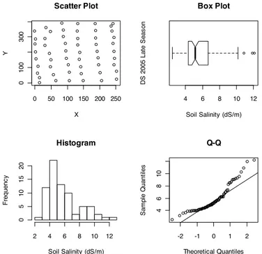
Soil salinity data collected in 17 fields in the downstream study area during the year 2008 are presented in this paper. Figures 2 and 3 show two examples of the data
distribution at the field scale. These figures show the scatter plots, box plots, histograms, and Q-Q plots. Scatter plots provide information about the spacing and distance between points. Histograms provide information about the mode, an indication of the overall variation, and the shape of the distribution, normal, or skewed. Box plots provide
information about the degree of dispersion, skewness, the middle 50% of the data, the 75th and 25th percentile of the data sets, the minimum and maximum data values, and the outliers. Q-Q plots provide information about the shape of the distributions (normal or skewed). The closer the points to the line, the closer the distribution is to a normal
distribution. The average distance between the collected soil salinity points is around 30 to 50 meters. The box plot, the histogram, and the Q-Q plot show that the data distribution in the first example is close to the normal distribution. In the second example, the distribution is skewed to the right which is supported by the shapes of the box plot, the histogram, and the Q-Q plot. The rest of the fields represent widely different cases for the spacing and distribution from normal, slightly right skewed, and sharply right skewed.
0 50 100 150 200 250 01 0 0 3 0 0 X Y 3.5 4.0 4.5 5.0 5.5 Soil Salinity (dS/m) DS 0 1 Histogram Soil Salinity (dS/m) Fr e q u e n c y 3.5 4.0 4.5 5.0 5.5 6.0 05 1 0 2 0 -2 -1 0 1 2 3. 5 4. 5 5. 5 Q-Q Theoretical Quantiles Sa m p le Q u a n ti le s
Figure 2. Scatter plot, box plot, histogram, and Q-Q plot for field DS 01 (close to normal distribution).
0 200 400 600 800 02 0 0 6 0 0 Scatter plot X Y 5 10 15 20 25 Box plot Soil Salinity (dS/m) DS 1 8 Histogram Soil Salinity (dS/m) Fr e q u e n c y 5 10 15 20 25 02 0 6 0 1 0 0 -3 -2 -1 0 1 2 3 51 0 1 5 2 0 2 5 Q-Q Theoretical Quantiles Sa m p le Q u a n ti le s
Figure 3. Scatter plot, box plot, histogram, and Q-Q plot for field DS 01 (right skewed distribution).
For the sub-basin scale, usually the data is collected at the early season during May and the late season during August. For this study three data sets were selected to be evaluated:
2004 early season, 2005 early season, and 2005 late season. These data sets were selected because they include the largest number of fields. Figure 4 represents one of the three selected sets, the 2005 late season. The scatter plot shows that the average distance among the values of the measured points in different fields is between 1,500 meters to 2,000 meters. The distribution is right skewed which is support by the box plot, the histogram and the Q-Q plot. The other two sets have similar average distance among the points and similar distribution. 0 50 100 150 200 250 01 0 0 3 0 0 Scatter Plot X Y 4 6 8 10 12 Box Plot Soil Salinity (dS/m) DS 2 0 0 5 L a te S e a s o n Histogram Soil Salinity (dS/m) Fr e q u e n c y 2 4 6 8 10 12 05 1 0 1 5 2 0 -2 -1 0 1 2 46 8 1 0 Q-Q Theoretical Quantiles Sa m p le Q u a n ti le s
Figure 4. Scatter plot, box plot, histogram, and Q-Q plot for field DS 2005 late season (right skewed distribution).
Table 1 shows the Moran’s I and Moran’s p-value (2-side) for measuring the
autocorrelation among the observed data for all individual fields and sub-basin data sets. The values of I vary from -1 to 1 while 1 means a perfect positive autocorrelation and -1 means a perfect negative autocorrelation. P-values of less than 0.05 mean the presence of autocorrelation while p-values of more than 0.05 mean no autocorrelation. For the field scale, all the individual fields show an existence of autocorrelation except for fields DS10 and DS21. There is no autocorrelation among the three data sets for the sub-basin scale. This is due to the large distance among the point.
4.2 Using IDW:
The goal of using inverse distance functions as estimators is to give more importance to the closest sampled points (Webster and Oliver, 2001). Power function values lower than one are closest to a simple average estimation (Isaaks and Srivastava, 1989). Integer power function values of 1, 2, 3, and 4, and 5 are the most commonly used in the literature (Kravchenco and Bullock, 1999). However, in this study, many cases were considered
using a number of neighbors of 4, 6, 8, 10, and 12 while optimizing the power function for each number of neighbors (using ArcGIS). Of all the cases considered, the one that
minimized the root mean square error was selected. The size of the neighborhood and the number of neighbors are also relevant to the accuracy of the results.
Table 1. Moran’s I and Moran’s p-value (2-side) for measuring the autocorrelation among the observed data for all individual fields and sub-basin data sets.
Field I P-value (2-side)
DS01 0.080 0 DS02 0.109 0 DS04 0.157 0 DS05 0.161 0 DS06 0.224 0 DS07 0.146 0 DS09 0.041 0 DS10 0.003 0.254 DS11 0.081 0 DS13 0.118 0 DS16 0.082 0.004 DS17 0.082 0 DS18 0.139 0 DS19 0.074 0 DS20 0.168 0 DS21 -0.084 0.7 DS22 0.100 0 DS2004 early season 0.002 0.448 DS2005 early season 0.010 0.272 DS2005 late season 0.006 0.71 4.3 Using OK:
Semivariograms describe the correlation in the data measured at sample locations. Exponential, Gaussian and Spherical models were fitted to the sample semivariograms using a weighted least-squares method (Robertson 1987). The semivariogram model with the smallest AICC (Akakie Information Corrected Criteria) was selected to describe the spatial dependencies in the soil salinity data. Nugget variance is the variance at zero distance, Sill is the lag distance between measurements at which one value for a variable does not influence neighboring values and Range is the distance at which values of one variable become spatially independent of another (Lopez-Granadoz et al. 2002). In this study, the number of neighbors was selected based on the number that minimizes the variance of the prediction. The lag size was selected to be closer to the average distance between the measured points and the number of lags was selected as the number of lags multiplied by the lag size which should be close to half the distance between the farthest pairs of points.
4.4 Model Evaluation:
Comparing the estimated values with the observed values as well as cross validation was used to evaluate the performance of both the IDW and OK techniques. Also, the
distributions and normality of the observed data and the predicted values using both the IDW and OK techniques were analyzed using the histograms, the box plots, and the Q-Q plots. The performance of both techniques, in terms of the accuracy of estimates, was assessed by comparing the deviation of the soil salinity estimates from the measured data through the use of cross-validation (Isaak and Srivastava, 1989; Webster and Oliver, 2001). In such a procedure, sample values are deleted from the data set, one at a time and then the value in turn is interpolated by performing the interpolation algorithm with the remaining sample values. This yields a list of estimated values of the variable data paired to those measured at sampled locations. In this study the comparison of the performance between the interpolation techniques was achieved by using the Mean Absolute Error (MAE) and the Root Mean Square Error (RMSE) (Zar, 1999).
5. Results
The distance between the soil salinity readings plays an important role in the
performance of the geostatistical models. For the field scale, the average distance among the soil salinity readings is between 30 meters and 60 meters, while the average distance among the mean values of the soil salinity readings in the selected fields for the sub-basin is from 1,500 meters to 2,000 meters. Smaller distances among the soil salinity readings at the field scale tend to generate more reasonable variograms. However, larger distances among the mean values of the soil salinity readings in the selected fields at the sub-basin scale makes it harder to generate reasonable variograms. The performance of kriging techniques depends mainly on the variograms. In this study three different variograms: spherical, Gaussian, and exponential were evaluated. The evaluation was based on the Akakie Information Corrected Criteria (AICC), the model that minimized the AICC value was selected. In most cases either at the field scale or sub-basin scale, the spherical model performed the best. Figure 5 shows three examples of variagram models for fields DS04, DS17 and DS20 for the field scale. The figure shows that for DS04 the spherical
variogram best fits the points then DS20 and last DS17. Figure 6 shows three examples of variagrams for the three sub-basin datasets. The figures show that the model does not fit well due to the large distance among the points which affects the performance of the OK model.
0 100 200 300 400 500 600 0. 0 0. 2 0. 4 0. 6 0. 8 xp yp DS04 0 100 200 300 400 500 0. 0 0. 2 0. 4 0. 6 0. 8 1. 0 xp yp DS17 0 200 400 600 800 02 468 1 0 xp yp DS20
Figure 5. The fitted spherical variogram model for the fields DS04, DS17, and DS20.
0 10000 20000 30000 40000 02 46 8 xp yp DS 2004 Early Season 0 10000 20000 30000 40000 01 2 3 xp yp DS 2005 Early Season 0 10000 20000 30000 40000 01 23 45 xp yp DS 2005 Late Season
Figure 6. The fitted spherical variogram model for the data sets of the sub-basin scale: for year 2004 early season, 2005 early season, and 2005 late season,
Figures 7, 8, and 9 show three examples for three different fields: DS04, DS17, and DS20. These fields were presented because they show different distributions. DS04 shows an example close to a normal distribution; DS17 shows a distribution slightly right skewed, and DS20 shows a distribution highly skewed to the right. The performance of IDW is slightly better than the performance of OK in field DS04. The performance of OK is slightly better than the performance of IDW in field DS17. The performance of both IDW and OK was very close in field DS20. Figure 10 shows the box plot, the histogram and the Q-Q plots for the 2004 early season dataset at the sub-basin scale. The figure shows that IDW outperformed the OK techniques which can be attributed to the lack of autorelation among the observed points (from 1,500 meters to 2,000 meters). Also the figure shows that the kriging underestimate the high estimated values which is clearly seen in the distance between the whiskers of the box plot.
3 4 5 6 7 Observed Soil Salinity (dS/m) DS 0 4 3 4 5 6 7 IDW Soil Salinity (dS/m) DS 0 4 3 4 5 6 7 OK Soil Salinity (dS/m) DS 0 4 Observed Soil Salinity (dS/m) Fr e q u e n c y 3 4 5 6 7 01 0 3 0 IDW Soil Salinity (dS/m) Fr e q u e n c y 3.0 4.0 5.0 6.0 01 0 3 0 OK Soil Salinity (dS/m) Fr e q u e n c y 3.0 4.0 5.0 6.0 01 0 3 0 -2 -1 0 1 2 34 5 6 7 Observed Theoretical Quantiles Sa m p le Q u a n til e s -2 -1 0 1 2 34 5 6 7 IDW Theoretical Quantiles Sa m p le Q u a n til e s -2 -1 0 1 2 34 5 6 7 OK Theoretical Quantiles Sa m p le Q u a n til e s
Figure 7. Comparison among the distributions of observed data, the predicted data using IDW, and the predicted data using OK for field US04 which is slightly right skewed.
3 4 5 6 7 8 Observed Soil Salinity (dS/m) DS 1 7 3 4 5 6 7 8 IDW Soil Salinity (dS/m) DS 1 7 3 4 5 6 7 8 OK Soil Salinity (dS/m) DS 1 7 Observed Soil Salinity (dS/m) Fr e q u e n c y 4 5 6 7 05 1 5 2 5 IDW Soil Salinity (dS/m) Fr e q u e n c y 4.0 4.5 5.0 5.5 6.0 6.5 7.0 05 1 5 2 5 OK Soil Salinity (dS/m) Fr e q u e n c y 4 5 6 7 05 1 5 2 5 -2 -1 0 1 2 34 5678 Observed Theoretical Quantiles Sa m p le Q u a n til e s -2 -1 0 1 2 34 5678 IDW Theoretical Quantiles Sa m p le Q u a n til e s -2 -1 0 1 2 34 5678 OK Theoretical Quantiles Sa m p le Q u a n til e s
Figure 8. Comparison among the distributions of observed data, the predicted data using IDW, and the predicted data using OK for field US17 which is close to a normal distribution.
0 5 10 15 20 25 30 Observed Soil Salinity (dS/m) DS 2 0 0 5 10 15 20 25 30 IDW Soil Salinity (dS/m) DS 2 0 0 5 10 15 20 25 30 OK Soil Salinity (dS/m) DS 2 0 Observed Soil Salinity (dS/m) Fr e q u e n c y 5 10 15 20 25 30 05 0 1 5 0 IDW Soil Salinity (dS/m) Fr e q u e n c y 5 10 15 20 25 05 0 1 5 0 OK Soil Salinity (dS/m) Fr e q u e n c y 5 10 15 20 25 05 0 1 5 0 -3 -2 -1 0 1 2 3 01 0 2 0 3 0 Observed Theoretical Quantiles Sa m p le Q u a n til e s -3 -2 -1 0 1 2 3 01 0 2 0 3 0 IDW Theoretical Quantiles Sa m p le Q u a n til e s -3 -2 -1 0 1 2 3 01 0 2 0 3 0 OK Theoretical Quantiles Sa m p le Q u a n til e s
Figure 9. Comparison among the distributions of observed data, the predicted data using IDW, and the predicted data using OK for field US20 which is highly skewed to the right.
0 2 4 6 8 10 Observed Soil Salinity (dS/m) DS 2 0 0 4 E a rl y S e a s o n 0 2 4 6 8 10 IDW Soil Salinity (dS/m) DS 2 0 0 4 E a rl y S e a s o n 0 2 4 6 8 10 OK Soil Salinity (dS/m) DS 2 0 0 4 E a rl y S e a s o n Observed Soil Salinity (dS/m) Fr e q u e n c y 2 4 6 8 10 05 1 0 1 5 2 0 IDW Soil Salinity (dS/m) Fr e q u e n c y 2 4 6 8 10 05 1 0 1 5 2 0 OK Soil Salinity (dS/m) Fr e q u e n c y 4.5 5.0 5.5 6.0 05 1 0 1 5 2 0 -2 -1 0 1 2 02 4 6 8 1 0 Observed Theoretical Quantiles Sa m p le Q u a n til e s -2 -1 0 1 2 02 4 6 8 1 0 IDW Theoretical Quantiles Sa m p le Q u a n til e s -2 -1 0 1 2 02 4 6 8 1 0 OK Theoretical Quantiles Sa m p le Q u a n til e s
Figure 10. Comparison among the distributions of observed data, the predicted data using IDW, and the predicted data using OK for the sub-basin scale for the 2004 early season.
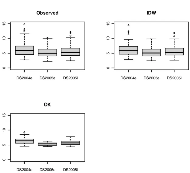
Figures 11 and 12 show the box plots of the observed and predicted data using IDW and OK for the three data sets at the sub-basin scale and the individual fields at the field scale respectively. Figure 11 shows the box plots for the three data sets that represent the sub-basin scale. The performance of IDW was better than the performance of OK. The OK underestimates the predicted values. The large distance among the observed data and the lack of autocorrelation violates the assumptions of OK which makes the model perform poorly. Figure 12 shows that there is no significant difference between the observed and predicted data using IDW and OK techniques. This means that with the small distance between samples and the existence of autocorrelation among the data, the performance of both IDW and OK is gets better.
5.1 Model Evaluation:
The MAE and the RMSE are used to evaluate the accuracy of the IDW and OK predictions. The MAE is similar to the RMSE but is less sensitive to large forecast errors. For small or limited data sets the use of MAE is preferred. The RMSE is the square root of the variance of the residuals. It indicates the absolute fit of the model to the data, how close the observed data points are to the model’s predicted values. Whereas R-squared is a relative measure of fit, RMSE is an absolute measure of fit. As the square root of a variance, RMSE can be interpreted as the standard deviation of the unexplained variance, and has the useful property of being in the same units as the response variable. Lower values of RMSE indicate a better fit.
DS2004e DS2005e DS2005l 05 1 0 1 5 Observed DS2004e DS2005e DS2005l 05 1 0 1 5 IDW DS2004e DS2005e DS2005l 05 1 0 1 5 OK
Figure 11. Comparing the observed data and the predicted data using IDW and Ok for three data sets for the sub-basin scale.
5.1.1 Comparing the observed and predicted values:
Table 2 shows the MAE and RMSE for comparing the observed and predicted values of IDW and OK for all individual fields and the three data sets of the sub-basin. The values of MAE and RMSE for the field scale are small and reasonable except for a few fields such as DS11 and DS22. There are a few fields where the MAE and the RMSE are slightly high for both the IDW and OK such as DS05, DS06, and DS07. In general, there is no
significant difference in the MAE and RMSE values between IDW and OK. However, for the sub-basin scale, the IDW outperformed the OK which can be contributed to the lack f autocorrelation among the data since the distance between the observed points is between 1,500 meters and 2,000 meters.
DS01 DS02 DS04 DS05 DS06 DS07 DS09 DS10 DS11 DS13 DS16 DS17 DS18 DS19 DS20 DS21 DS22 51 0 1 5 2 0 2 5 3 0 DS01 DS02 DS04 DS05 DS06 DS07 DS09 DS10 DS11 DS13 DS16 DS17 DS18 DS19 DS20 DS21 DS22 51 0 1 5 2 0 2 5 DS01 DS02 DS04 DS05 DS06 DS07 DS09 DS10 DS11 DS13 DS16 DS17 DS18 DS19 DS20 DS21 DS22 51 0 1 5 2 0 2 5
Figure 12. Comparing the observed data and the predicted data using IDW and Ok for all individual fields in the field scale.
Table 2. MAE and RMSE for comparing the observed and predicted values of IDW and OK for all individual fields and the three data sets of the sub-basin.
Field IDW OK
MAE RMSE MAE RMSE
DS01 0.08 0.10 0.12 0.15 DS02 0.00 0.03 0.05 0.06 DS04 0.00 0.23 0.16 0.25 DS05 0.01 1.34 1.14 1.72 DS06 0.00 1.23 0.53 0.97 DS07 0.00 1.43 1.04 1.50 DS09 0.00 0.61 0.46 0.82 DS10 0.00 0.03 0.07 0.08 DS11 0.04 2.08 1.73 2.57 DS13 0.01 0.22 0.12 0.19 DS16 0.00 0.03 0.14 0.22 DS17 0.00 0.39 0.13 0.20 DS18 0.00 0.49 0.12 0.45 DS19 0.00 0.52 0.26 0.44 DS20 0.00 0.58 0.39 0.79 DS21 0.00 0.03 0.04 0.05 DS22 0.03 2.14 0.78 1.27 DS2004 early season 0.11 0.17 1.54 2.01 DS2005 early season 0.06 0.08 1.19 1.55 DS2005 late season 0.09 0.13 1.37 1.81 5.1.2 Cross validation:
Cross validation is as important as comparing the predicted values with the observed ones. Table 3 shows the cross validation results for IDW and OK for all individual fields and the three data sets of the sub-basin. The MAE the RMSE values are used to measure the differences between values predicted by the IDW and OK models and the observed values. For the field scale the MAE values for both IDW and OK are close to zeros except for field DS22 when using IDW. For almost half of the fields the values of RMSE are very small (less than 0.5). Six fields have values larger than one. Similarly to the previous table, fields DS11 and DS22 show the worst results for both IDW and OK. In general the results shown in Table 3 are very similar to the results from Table 2. However, in contrast to Table 2, the results for the sub-basin scale show that there is no significant difference in the values of MAE and RMSE. This means that the IDW was significantly better than the OK in estimating the values from the observed data but are similar to the OK values in terms of cross validation. Therefore, as presented earlier and cited from the literature, this reduces the overall performance of the IDW method.
Figure 13 shows the generated maps of soil salinity predicted surfaces using IDW and OK for fields DS04, DS17, and DS20 at the field scale. The 3-D maps were selected to show the generated maps for both IDW and OK because they has the option of adding the observed points to the surface which makes it easier to compare the results of both models with the observed values. The figure shows that there is no significant difference between both predicted surfaces using the IDW and OK techniques. In general there are some spikes in the generated surfaces using IDW while the surface generated using OK is
smoother. Even though these three fields presented in the figure have different
distributions these distributions do not have significant impact on the results of models.
Table 3. MAE and RMSE values of the cross validation results for comparing the performace of the IDW and OK for all individual fields and the three data sets of the sub-basin.
Field IDW OK
MAE RMSE MAE RMSE
DS01 0.001 0.345 0.001 0.352 DS02 0.011 0.349 0.001 0.360 DS04 0.049 0.508 0.005 0.491 DS05 0.037 2.316 0.001 2.287 DS06 0.145 2.074 0.009 1.958 DS07 0.018 1.719 0.002 1.703 DS09 0.004 1.006 0.004 1.077 DS10 0.014 0.394 0.011 0.414 DS11 0.171 4.270 0.030 4.281 DS13 0.017 0.473 0.005 0.454 DS16 0.029 0.380 0.011 0.410 DS17 0.004 0.756 0.002 0.773 DS18 0.005 2.076 0.008 1.980 DS19 0.021 0.755 0.002 0.736 DS20 0.046 1.587 0.005 1.565 DS21 0.009 0.590 0.042 0.618 DS22 0.276 4.667 0.094 4.660 DS2004 early season 0.055 2.535 0.093 2.574 DS2005 early season 0.019 1.748 0.007 1.698 DS2005 late season 0.042 2.190 0.067 2.122
Figure 14 shows the generated maps of the soil salinity predicted surfaces using IDW and OK for the three data sets in the sub-basin scale. The figure shows a significant difference between both predicted surfaces using the IDW and OK techniques. The IDW outperformed the OK in estimating values from the observed data. The OK tends to be smoother than the IDW which makes it under estimate the high values. As in the previous figure there are some spikes in the surface generated using the IDW. In this figure the contribution of sampling density or spacing between samples is very significant. The large sampling spacing (1,500 meters to 2,000 meters) makes the performance of OK worse than the performance of IDW. However, as concluded in Tables 2 and 3, it is not enough to evaluate the model performance only through the estimated values. The cross validation results show that both model performances are almost the same in this case which makes the overall performance of OK similar to the performance of IDW.
X 0 200 400 600 Y 0 200 400 600 S o il S a lin ity (dS /m ) 3 4 5 6 7 X 0 200 400 600 Y 0 200 400 600 S o il S a lin ty (dS /m ) 3 4 5 6 7 X 0 100 200 300 400 500 Y 0 100 200 300 400 S o il S a lin ty (dS /m ) 4 5 6 7 X 0 100 200 300 400 500 Y 0 100 200 300 400 S o il S a lin ity (d S /m ) 3 4 5 6 7 X 0 200 400 600 800 Y 0 500 1000 1500 S o il S a lin ty (dS /m ) 5 10 15 20 X 0 200 400 600 800 Y 0 500 1000 1500 S o il S a lin ity (d S /m ) 5 10 15 20
Figure 13. Generated maps of soil salinity predicted surfaces using IDW and OK for fields DS04, DS17, and DS20 at the field scale.
DS 2004 Early Season (IDW) DS 2004 Early Season (OK)
DS 2005 Early Season (IDW) DS 2005 Early Season (OK)
DS 2005 Late Season (IDW) DS 2005 Late Season (OK)
X 0 10000 20000 30000 40000 50000 Y 0 5000 10000 15000 20000 S o il S a lin ty (dS /m ) 0 5 10 15 X 0 10000 20000 30000 40000 50000 Y 0 5000 10000 15000 20000 S o il S a lin ity (d S /m ) 0 5 10 15 X 0 10000 20000 30000 40000 Y 0 5000 10000 15000 S o il S a lin ty (dS /m ) 3 4 5 6 7 8 9 X 0 10000 20000 30000 40000 Y 0 5000 10000 15000 S o il S a lin ity (dS /m ) 3 4 5 6 7 8 9 X 0 10000 20000 30000 40000 50000 Y 0 5000 10000 15000 S o il S a lin ty (d S /m ) 4 6 8 10 X 0 10000 20000 30000 40000 50000 Y 0 5000 10000 15000 S o il S a lin ity (dS /m ) 4 6 8 10
Figure 14. Generated maps of soil salinity predicted surfaces using IDW and OK for the three sets at the sub-basin scale.
6. Conclusions
The distance between points, the data distribution, and the autocorrelation were set as parameters to evaluate both IDW and OK techniques. The different data sets presented in this study for both the field scale and sub-basin scale show different spacing among the points, different data distributions, and different autocorrelations. The results of this study indicate that there is no significant difference in the performance of both geostatistical and deterministic techniques at the field scale. However, the performance of the deterministic technique was significantly better than the geostatistical technique at the sub-basin scale from the point of view of estimating values from the observed data. However, the overall performance depends not only on the estimated values but also on the cross validation. The OK technique tends to be smoother than the IDW technique which makes it under estimate the high values. The contribution of autocorrelation was not significant which can be attributed to existence of autocorrelation but it is not significant. Also, for the field scale, the sampling density does not have a significant impact on the results of the models. This also can be attributed to the fact that both models perform better when samples are closer. Even though the contribution of sampling density or spacing was not significant on the field scale, it was very significant at the sub-basin scale. The large sampling spacing (1,500 meters to 2,000 meters) makes IDW outperformed OK from the point of view of
estimating soil salinity values. However, the cross validation results show that both model performances are almost the same for the sub-basin scale.
References
Corwin, D.L., Lesch, S.M., 2003. Application of soil electrical conductivity to precision agriculture: Theory, principles and guidelines. Agronomy Journal 95, 455–471.
Dalthorp, D., J. Nyrop and M. Villani, 1999. Estimation of local mean population densities of Japanese beetle grubs (Scarabaeidae: Coleoptera). Environ. Entomol.Apr. 28: 255-265.
Deutsch, C. V., and Journel, A. G. (1998). GSLIB, Geostatistical software library and user’s guide, 2nd Ed., Oxford University Press, New York.
Gotway, C.A., R.B. Ferguson, G.W. Hergert and T.A. Peterson, 1996. Comparison of kriging and inverse-distance methods for mapping soil parameters. Soil Sci. Soc. Am. J., 60: 1237-1247.
Hosseini, E., J. Gallichand and D. Marcotte, 1994. Theoretical and experimental performance of spatial interpolation methods for soil salinity analysis. Trans. ASAE, 37: 1799-1807.
Isaaks, E.H. and R.M. Srivastava, 1989. An Introduction to Applied Geostatistics. Oxford University Press, New York, pp: 561.
Kollias, V.J. 1999. Mapping the soil resources of a recent alluvial plain in Greece using fuzzy sets in a GIS environment. J. Soil Sci. 50:261–273.
Kravchenko, A.N. 2003. Influence of spatial structure on accuracy of interpolation methods. Soil Sci. Soc. Am. J. 67:1564–1571.
Kravchenko, A.N. and D.G. Bullock, 1999. A comparative study of interpolation methods for mapping soil properties. Agron. J. 91:393–400.
Lapen, D.R. and H.N. Hayhoe, 2003. Spatial analysis of seasonal and annual temperature and precipitation normals in Southern Ontario, Canada. J. Great Lakes Res., 29: 529-544.
Laslett, G.M. 1987. Comparison of several spatial prediction methods for soil pH. J. Soil Sci. 38:325–341. Lopez-Granados, F., M. Jurado-Exposito, S. Atenciano, A. Ferrer, M.S. de la Orden and L. Garcia-Torres, 2002. Spatial variability of agricultural soil parameters in Southern Spain. Plant Soil, 246: 97-105.
Matheron, G., 1971. The Theory of Regionalized Variables and its Applications. Ecole des Mines, Fontainebleau, France, pp: 211.
Miller, J., Franklin, J., and Aspinall, R. (2007). “Incorporating spatial dependence in predictive vegetation models.” Ecol. Modell., 202:3(4), 225–242.
Mueller, T.G. 2004. Site-specific fertility management: A model for predicting map quality. Soil Sci. Soc. Am. J. 68:2031–2041.
Mueller, T.G., F.J. Pierce, O. Schabenberger and D.D. Warncke, 2001. Map quality for site-specific fertility management. Soil Sci. Soc. Am. J., 65: 1547-1558.
Nalder, I.A. 1998. Spatial interpolation of climatic normals: Test of a new method in the Canadian boreal forest. Agric. Forest Meteor. 92:211–225.
Olea, R. A. (1991). Geostatistical glossary and multilingual directionary, Oxford University Press, New York.
Pozdnyakova, L., and Zhang, R. (1999). “Geostatistical analyses of soil salinity in a large field.” Precis. Agric., 1, 153–165.
Rhoades, J.M., Chanduvi, F., Lesch, S.M., 1999. Soil salinity assessment. Methods and interpretation of electrical conductivity measurements. FAO Irrigation and Drainage Paper 57. FAO, Rome, 150pp. Samra, S., and Gill, H. S. (1993). “Modeling of variation in a sodium contaminated soil and associated tree
growth.” Soil Sci., 155(2), 148.
Schloeder, C.A. 2001. Comparison of methods for interpolating soil properties using limited data. Soil Sci. Soc. Am. J. 65:470–479.
Tabios, G.Q. 1985. A comparative analysis of techniques for spatial interpolation of precipitation. Water Resour. Bull. 21:365–380.
Triantafilis, J., Odeh, I. O. A., and McBratney, A. B. (2001). “Five geostatistical models to predict soil salinity from electromagnetic induction data across irrigated cotton.” Soil Sci. Soc. Am. J., 65, 869–878. Utset, A., Ruiz, M. E., Herrera, J., and Ponce de Leon, D. (1998).“A geostatistical method for soil salinity
sample site spacing.” Geoderma, 86, 143–151.
Wartenburg, D. 1991. Estimating exposure using kriging: A simulation study. Environ. Health Perspect. 94:75–82.
Weber, D. 1992. Evaluation and comparison of spatial interpolators. Math. Geol. 24:381–391
Weisz, R. 1995. Map generation in high-value Horticultural Integrated Pest Management: Appropriate Interpolation Methods for Site- specific pest management of Colorado potato beetle (Coleoptera: Chrysomelidae). J. Econ. Entomol. 88:1650–1657.