AN ALGORITHM FOR THE NEAR OPTIMIZATION OF TACTICAL FORCE RATIOS IN THE DEFENSE by Mark E. Tillman
ARTHUR LAZES LIBRARY COLOBW&DO SCSSOOL o i MINES
ProQuest N um ber: 10783681
All rights reserved INFORMATION TO ALL USERS
The qu ality of this repro d u ctio n is d e p e n d e n t upon the q u ality of the copy subm itted. In the unlikely e v e n t that the a u th o r did not send a c o m p le te m anuscript and there are missing pages, these will be note d . Also, if m aterial had to be rem oved,
a n o te will in d ica te the deletion.
uest
ProQuest 10783681
Published by ProQuest LLC(2018). C op yrig ht of the Dissertation is held by the Author. All rights reserved.
This work is protected against unauthorized copying under Title 17, United States C o d e M icroform Edition © ProQuest LLC.
ProQuest LLC.
789 East Eisenhower Parkway P.O. Box 1346
A thesis submitted to the Faculty and the Board of Trustees of the Colorado School of Mines in partial fulfillment of the requirements for the degree of Master of Science (Mathematics). Golden, Colorado Date < V feJ> 7 / Signed: Mark E. Tillman Golden, Colorado Date /I f & t L f f Approved: fnr. R .E .D . W o o lseji-o T Thesis Ac Dr. Ardel J. Boes Professor and Head
Department of Mathematics and Computer Sciences
T-4002
ABSTRACT
This thesis contains a method which positions tactical units in a defensive posture against an enemy force. The positioning criterion used is one which minimizes the ratio of enemy force to friendly force. Across the battle area this method minimizes the sum of all ratios of enemy to friendly forces.
The problem of matching units to oppose each other is one of particular importance at the Division and Corps level. Here, as part of the military planning process, staffs
analyze different dispositions of friendly forces for the commander. Currently neither the staff nor the commander formulate an option which best minimizes the ratio of forces. One possible reason to avoid this type of formulation is that the mathematics required for solution is not simple. Ironically, though, this ratio of force weighs heavily on the
decision of which option to implement. This thesis offers a simple method that nearly minimizes the ratio of forces. The method maximizes the differential between potential force ratios that could result should units be assigned to oppose each other. A very good solution results in as many iterations as units to be assigned.
As a result of using this method, the commander could choose an option which incorporates the critical decision criterion of force ratio in its formulation. With this course of action as a standard, the commander and his staff can further identify potentially critical flaws in defenses.
TABLE OF CONTENTS
Ease
ABSTRACT... iii
LIST OF FIGURES AND TABLES ... vi
ACKNOWLEDGEMENTS ... vii
Chapter 1. BACKGROUND AND ANNOTATED BIBLIOGRAPHY ... 1
1.1 Military Literature Review ... 1
1.2 Mathematical Literature Review ... 4
1.3 Summary of Research ... ... 4
Chapter 2. PROBLEM DEFINITION AND SOLUTION TECHNIQUE ... 6
2.1 Problem Background and Discussion ... 6
2.2 Assumptions ... 7
2.3 Limitations ... 7
2.4 Solution Methods ... 8
2.4.1 Fractional Integer Programming Method ... 9
2.4.2 The Near-Minimal Algorithm ... 12
2.5 Method Overview ... 14
Chapter 3. PROBLEM AND SOLUTION METHOD ... 15
3.1 The Military Problem ... 15
3.2 The Integer Program Formulation ... 19
3.3 Integer Program Problem Solving Procedure ... 20
3.3.1 Maximizing the Denominator... 24
3.3.2 Minimizing the Numerator... 27
3.4 Procedure for the Near-Minimal Algorithm... 29
Chapter 4. EXAMPLE PROBLEMS ... 38
4.1 Example 1 (Using Fractional Integer Programming)... 38 iv
T-4002
4.1.1 Problem Statement... 38
4.1.2 Fractional Integer Program Formulation... 38
4.1.3 Integer Programming Procedure... 39
4.1.4 Conclusions ... 45
4.2 Example 2 (Use of the Near-Minimal Algorithm)... 47
4.2.1 Problem Statement... 47
4.2.2 Problem Discussion... 49
4.2.3 Application of the Near-Minimal Algorithm... 49
4.2.4 Conclusions ... 60
4.3 Example 3 (Summarized Use of the Near-Minimal Algorithm) 62 4.3.1 Problem Statement ... 63
4.3.2 Problem Discussion... 65
4.3.3 Conclusions ... 65
4.4 Example 4 (Using the Analogous Computer Program) ... 67
4.4.1 Problem Statement... 67
4.4.2 Problem Discussion... 67
Chapter 5. CONCLUSION AND SUGGESTIONS FOR FURTHER RESEARCH... 69
5.1 Conclusion ... 69
5.2 Suggestions for Further Research... 70
SELECTED BIBLIOGRAPHY... 74
Appendix A: SOLUTION SET SIZES ... 76
Appendix B: BLANK FO RM S... 78
Appendix C: SAMPLE COMPUTER RUNS ... 81
Appendix D: ALGORITHM ANALYSIS... 86
Appendix E: COMPUTER PROGRAMS... 90 v
LIST OF FIGURES AND TABLES
Figure Page
2.1 Solution Set S izes... 10
2.2 Integer Program Computer Run Times ... 12
2.3 Near-Minimal Algorithm Computer Run Tim es... 13
3.1 Simplified Military Situation ... 16
3.2 Expanded Military Situation... 18
3.3 Fractional Integer Program Flowchart... 21
3.4 Exploded Worksheet R ow ... 31
3.5 Near-Minimal Algorithm Flowchart ... 32
4.1 Example 1 Degeneracy... 43
4.2 Example 2 Situation ... 48
4.3 Algorithm Worksheet Preparation ... 50
4.4 Algorithm Worksheet Iteration 1 ... 52
4.5 Algorithm Worksheet Iteration 2 ... 54
4.6 Algorithm Worksheet Iteration 3 ... 56
4.7 Algorithm Worksheet Iteration 4 ... 58
4.8 Algorithm Worksheet Iteration 5 ... 61
4.9 Example 2 Final Assignments... 62
4.10 Examples 3 and 4 Situation ... 64
4.11 Example 3 Completed Worksheet ... 66
4.12 Computer Program Example... 68
B -l Near-Minimal Algorithm Worksheet ... 79
B-2 FORM 86-(F626)-3352 ... 80
Table Page 3.1 Double Product Truth Table... 25
4.1 Types and Numbers of Constraints and Variables ... 46
A -l Combinatoric Solution Set S izes... 77
D -l Analysis of Sample Problems... 88
T-4002
ACKNOWLEDGEMENTS
As with any effort of this magnitude, the end product would not be possible without the help of many people. I would like to thank just a few.
Giving more than just time and knowledge, was my academic advisor, Dr. Robert E. D. Woolsey. Dr. Woolsey gave me direction and wisdom during many hours of
consultation both in and out of the classroom. To him I am deeply indebted for having shared this experience.
I would also like to recognize Dr. Ruth Maurer and LTC Bruce Goetz. Each aided me invaluably in the production of this work. Through several months, they cheerfully reviewed my drafts and added constructive comments which added credibility to this document in both academic and military circles. To them I am grateful.
Thanks also goes to my brother, Mike, who, as a professional writer, reviewed my final draft. He certainly deserves many thanks.
Thanks, too, goes to my many friends here at school. Kevin Loy, Joe Huber, Jim Watson, and Doug Hart are just a few. Each gave valuable time to me and this work.
Critical in almost everything I have done in life are my parents. In this endeavor they contributed most notably with a direct contribution to my education. The very computer that this work was completed on was a result of a monetary, interest free, loan from my loving parents. Someday I hope to be rich enough to repay the note. Until then I know this thank you will suffice.
Finally, to my wife, Sallie, I sincerely apologize for letting this academic pursuit interfere with our family life. She has been, as always, unflinchingly supportive in
everything I have done. Thank you for giving totally of your time, patience, and love. I know she will accept our diploma as witness to her sacrifices over the past two years of "mind-boggling" math.
T-4002 1
Chapter 1
BACKGROUND AND ANNOTATED BIBLIOGRAPHY
This thesis is centered around two problems. The first problem is the military problem. Simply put, this problem is the determination of which friendly units should be assigned opposite which enemy units so that the ratio of forces is minimized. The second problem is the mathematical one which underlies the military one. The mathematical problem can be formulated using integer programming. Integer programming is sometimes used as a mathematical tool to optimize decision making. As it turns out, integer programming itself cannot be directly applied to the military problem. Instead, fractional integer programming is required to properly capture the military problem with
a mathematical decision means.
1.1 Military Literature Review
First, some background on the military problem. Interestingly, at the unclassified level, no previously published research is available. In the summer of 1990 this problem was researched for several weeks at the Command and General Staff College’s Combat Arms Research Library (CARL) at Fort Leavenworth, Kansas. The pursuit for related research included on-line subject, topic, and key word searches in the following data bases: the Defense Technical Information Center (DTIC) which includes over 2 million Department of Defense (DOD) documents; the National Technical Information Service (NTTS) which includes over 200,000 technical documents; and DIALOG which is mostly an applied science data base. Most references found in this search related to studies of simulation results from JANUS (an interactive simulation model currendy used by the
Army) and results of full scale force-on-force battles at the National Training Center (NTC). Statistical in nature, none of these studies related to the problem statement considered here. Additionally, several card catalogs at CARL were examined, which refer to information not available on any national on-line data base. These references included a general book collection of over 116,000 military works; a specialized
reference collection of military theses, dissertations, student papers, contract studies, and past research efforts; historical military documents from World War II, Korea, and Vietnam; the Combined Arms Center and Command and General Staff College archive collection which contains documents dated before the Civil War; and Army
administrative publications (both current and obsolete). In fact, absolutely no information related to the problem of minimizing the ratio of forces prior to conducting a simulation or full scale battle was found in this search.
The problem was also posed to several senior officers at the Army’s think tank of subject matter experts at the Center for Army Tactics. One officer, Lieutenant Colonel Pamperl, a senior tactics instructor at the Command and General Staff College, was able to confirm what was becoming a growing suspicion. He stated that the Army has yet to seriously address the problem of minimizing the ratio of forces prior to war fighting.
Several reasons may be cause for this. First, other, more significant factors, so it is hypothesized, may be more critical to success or failure on the battlefield. Many times, human factors may be more important than the number and disposition of tanks or tubes or artillery on the battlefield. This is certainly valid considering the myriad of factors that influence the outcome of battle. Second, the Army presently has a simple system that works.
T-4002 3
The current system is outlined in the Command and General Staff College’s text CGSC ST 100-9, The Command Estimate. The doctrine outlined in this text calls for the recommendation of the staff as to which of several proposed dispositions is the one the commander should subsequently war game or possibly war fight Mathematical
optimality may not exist in this set of proposed courses of action because each course of action was derived using experience and other intangibles not related to a systematic method of mathematical foundation. Given the enemy disposition, the proposed courses of action are a best guess on friendly force alignment. The decision criterion of force ratios is a tool only considered after the fact and not during course of action development. The final recommendation, however, is based on analyzing the relative combat power of friendly versus enemy forces. This analysis is performed on Form 86-(F626)-3352 (see Appendix B, Figure B-2). After determining the status and capabilities of units, the staff uses this form to make the calculations for relative combat power and force ratios.
Army doctrine stresses that decisions should not be based on force ratios alone (CGSC ST 100-9 [pg 3-2]). Analyzing relative combat power provides conclusions about friendly and enemy capabilities relative to the operation being planned. The comparison of forces provides the planner with a notion of "what to" (capabilities) and not "how to" (operations) fight. The author based the mathematical problem on this notion of "what to" fight. By so doing the force ratio criterion becomes part of the development process for the course of action.
The mathematical problem was formulated as an integer assignment program. Similar to traditional integer assignment problems, this problem seeks to determine which units the commander could assign against which enemy units. Unlike traditional
assignment problems, the objective in this problem is fractional. The fractions represent the force ratios. The next research effort was aimed at optimizing a fractional integer objective function subject to linear assignment constraints.
1.2 Mathematical Literature Review
Surprisingly, very little research was found in the area of fractional programming. A search for all articles related to fractional programming in The Institute of
Management Sciences, OR/MS Index. 1952-1987, was conducted. As many as ten or so articles in various journals were written over the past 25 or so years, yet after reviewing each, none were found related to the mathematical problem proposed. In every case, the fractional programming technique discussed applied to linear variables and not integer ones. Exploration of the School of Mines Library produced several titles relating to discrete optimization methods, applied combinatorics, and integer programming but none discussed fractional integer programming. Finally a search was conducted on an on-line Colorado State Library System at four different universities within Colorado. These were: the University of Colorado at Boulder, the University of Colorado at Denver, Colorado State University, and the University of Denver. Several promising titles were located in the Math and Business Libraries at UC Boulder. Unfortunately, none addressed a method for solving the fractional integer program.
1.3 Summary of Research
In summary, the background research for this thesis was extensive and
exhaustive. No previously published research on this problem was discovered within the scientific, mathematical, or military communities.
T-4002 5
Currently Army doctrine does not call for a mathematically optimal solution to the force ratio alignment problem (CGSC ST100-9 [pg 3-4]). However, by analyzing relative combat power as part of the course of action development process the staff could provide the commander a feel for near minimal relative strength ratios as a basis and standard for possible force alignment.
Chapter 2
PROBLEM DEFINITION AND SOLUTION TECHNIQUE
2.1 Problem Background and Discussion
Commanders and staff officers on today’s batdefield are faced with an extremely complex environment The ever-changing technologies serve to make every thought action, decision, and disposition of each unit vital. Indeed, the unit that is led and served by the best commanders and staff has the advantage from the outset. When time permits and before men and equipment are committed to a particular strategy, commanders and staffs war game different options for aligning units.
This war gaming is simply a process of thinking systematically about various courses of action and the ensuing chain of events. Prior to beginning this war gaming process, both the commander and staff each analyze the various proposed courses of action for troop alignment. This analysis is known as the estimate of the situation. The estimate is a critical procedural step in the military decision making process. The
estimate is normally performed by the staff officers and the commander of the unit. Each section chooses the course of action that best aligns forces against an expected enemy disposition. The decision tool currently used by the G2 (Division or Corps Intelligence Officer) and the G3 (Division or Corps Operations Officer) relies heavily on the concept of tactical force ratios. The tactical force ratio is determined by first assigning relative combat power indices (a number quantifying combat power relative to a fixed standard) to both friend and foe that the staff and commander feel will oppose each other at the onset of the battle (CGSC ST 100-9 [pg 3-3]). Simple division produces the force ratio. When the calculations are finished ihe staff draws conclusions about friendly and enemy
T-4002 7
capabilities and limitations. The force ratio calculations serve as a discriminating or screening criterion for the staff. Courses of action with unfavorable force ratios are possibly eliminated. Whereas courses of action with strong force ratios are favored and given further consideration. Based, in part, on these ratios the G3 recommends a course of action as the initial array of force to begin the war gaming process.
Historically a defender would need at least a ratio of 1 to 3 over an attacker to expect to defend terrain successfully.
2.2 Assumptions
Several assumptions are necessary before a solution method is established. First, an estimate of enemy force concentrations must be known. This in necessary to quantify enemy potential along each of the avenues of approach. Second, the friendly mission is a defensive one. Offensive operations do not directly apply the force ratio analysis in the detail discussed in this thesis. Third, an equal importance is given to the defense of each enemy avenue of approach. Otherwise, a weighting scheme is necessary. Finally, a correlation exists between force ratio minimization and increased success on the battlefield. Without this association these procedures are not applicable to decision making.
2.3 Limitations
For the purpose of this thesis several limitations exist. First, only unclassified information will be discussed and used. Classified sources are not necessary to develop or validate the methods discussed in this thesis. Second, the solution methods discussed in this thesis are of mathematical make-up. This is not an oversight or an omission of
other, possibly more effective, analysis techniques. The objective of this thesis was to identify mathematical methods and tools that could be used to assist staffs and
commanders in solving the problem of where to initially deploy units in the defense. The decision criterion used was one of minimizing the ratio of force while adhering to limited tactical prerequisites which will be discussed in chapter 3. The author did not model human factors which could be extremely relevant to the outcome of any battle. Nor did he attempt to simulate a dynamically changing scenario. This author does not intend for the method discussed in this thesis to replace the process currently used by staffs and
commanders. Instead, the product of this thesis can be used in conjunction with current Army staff planning doctrine to produce a better, more informed decision.
2.4 Solution Methods
This thesis will focus on two mathematical methods for solving the military problem. The first method formulates a fractional integer program which will determine an optimal solution to the mathematical objective. Two features of this technique will become apparent during its formulation. First, the procedure expends considerable time and effort. Second, the procedure is beyond the expertise of the typical staff officer who might be tasked to propose an array of forces. The second method discussed in this thesis is simple, quick, and persuasive. Furthermore, this second method will determine a near optimal course of action based on the tactical force ratio criterion in a fraction of the time needed to determine optimality using the first method. Once this near optimal course of action is determined, it could supplement the original courses and be analyzed further for practicality. By so doing, the commander could consider a course of action that includes the best available tactical force ratios as the basis for its formulation.
T-4002 9
2.4.1 Fractional Integer Programming Method
The problem of optimizing force alignments will be shown to be a fractional integer programming problem. This program has an objective function that is the sum of variable fractions (see eq. 2.1). In this formulation, the objective function would take the form:
I = i a,
Where the denominators 0, are defined as:
m
for each i, X ex.: — a,
7 = 1
Each term in the objective function represents the fractional ratio of force indices for a particular location on the battle front known as an avenue of approach. The
numerators of each of the ratios in the objective function (see eq. 2.1) are constant. Each of these constants represents the sum of the enemy combat power indices for a particular avenue of approach. At feasibility, the denominators of these ratios are all non-zero and represent a linear combination of the friendly combat power indices of units chosen to oppose the enemy at a particular avenue of approach. The decision variables x# represent the decision to assign a unit against an avenue of approach. These decision variables are found in the denominators of the ratios of the terms in the objective function. Each decision variable is constrained so that it may be used only once.
The constraints on the variables are similar to the traditional assignment or transportation problem. Initially all the decision variables are 0-1. The variable is equal to 1 if it is assigned to a term in the objective function (a particular avenue of approach). The constraint set for this formulation is shown below.
Subject to:
m
for each i , X ^ 1
j =i
n
for each j , "Lxu = l « = i 7
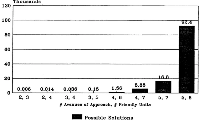
Surprisingly enough, this type of problem is not an easy one to optimize using known integer techniques or linear programs. Figure 2.1 illustrates the magnitude of the solution set size for problems of varying sizes. The combinatoric analysis used to
determine each solution set size is given in Appendix A, Table A-l.
T h o u s a n d s 120 100 80 60 40 20 5 .8 8 1.56 2, 3 2, 4 3, 4 3, 5 4, 6 4, 7 5. 7 5, 8 # A v en u es o f A p p ro a c h , § F rie n d ly U n its H H P o s s ib le S o lu tio n s
T-4002 11
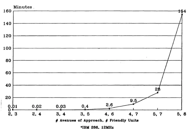
The difficulties in solving such a problem are two-fold. First, the objective function is non-linear. Attempts to linearize the objective function create many new variables and constraints. Second, many of the new variables introduced are not 0-1 like the original variable set. In the end, the program includes not only 0-1 variables, but also integer positive and strictly positive variables. This mixture limits the efficiency of known methods. The time required to formulate and solve the military problem with a fractional integer program may not always be practical. Depicted in Figure 2.2 is the possible solution time for problems of varying sizes. This time does not include time to formulate the problem. The solution times for the problems with four and five avenues of approach were extrapolated from run times for smaller sizes.
Nevertheless, a detailed discussion for this fractional integer formulation and a solution method is discussed in Chapter 3. If time and expertise are not available to address the military problem with a fractional integer programming solution or if an optimal solution is not absolutely necessary, then an approximately optimal result may be preferable.
I n te g e r S o lu tio n ( r u n tim e * ) M i n u t e s . 160 140 12 0 10 0 80 60 40 20 2 .6 0.4 0 .0 2 0 .0 3 2, 3 2. 4 3. 4 3. 5 4. 6 4, 7 5. 7 5, 8 § A v en u es o f A p p ro a c h , # F rie n d ly U n its •IBM 286, 12MHz
Figure 2.2: Integer Program Computer Run Times
2.4.2 The Near Minimal Algorithm
The algorithm presented in this thesis will determine a near minimum value for the fractional programming problem o f the type required to align defensive forces optimally. The algorithm can assign as many as "m" friendly units in no more than "m" iterations. The resulting solution is very close to the minimal value for the fractional integer program. Figure 2.3 reveals the average solution time for problems of varying sizes using the Near-Minimal Algorithm.
T-4002 13 A lg o rith m S o lu tio n ( r u n tim e * ) S e c o n d s 0 .3 5 0 .3 2 3 0 .3 0 .2 5 0.2 0.1 5 7 0 .1 5 o.ia 97 0.1 0 .0 5 3. 4 3. 5 5, 7 5. 8 2, 3 2. 4 4, 6 4, 7 # A v en u es o f A p p ro a c h , # F rie n d ly U n its •IBM 2 8 6 , 12MHz
Figure 23: Near-Minimal Algorithm Computer Run Times
Note the magnitude of difference in computer run time for each problem when the algorithm run time is compared to the integer program solution time. The near-minimal algorithm produces a very good solution in less than a half of a second. In contrast, the optimal solution may take hours to determine. The time savings is even more apparent when we consider the reality that the problem sizes here are smaller than those expected to be solved by staffs of a Division or Corps. There, the actual size may be eight or more avenues of approach and as many as 20 or so friendly units.
The efficiency of the algorithm is in its execution. Simply stated, the algorithm maximizes the differential between a previous infeasible upper bound solution and a
potential new upper bound solution which in also infeasible until the algorithm’s final iteration.
The algorithm proceeds by assigning variables to an appropriate term in the objective function. The choice of which term is made by comparing the marginal difference between the previous upper bound for that term and a new one should the variable be assigned to that term. The greatest marginal difference earns the variable for the term thereby eliminating it from being further assigned to another term. Each
iteration moves the objective function non-increasingly toward a newer and lower integer upper bound which is equal to or less than the previous one. At the conclusion of the algorithm, the final integer upper bound is feasible. This final upper bound is very near to the least upper bound for the objective function. At conclusion, the algorithm
successfully assigns friendly units to locations where the sum of the resulting force ratios is near-optimal.
2.5 Method Overview
In the pages that follow the reader will find two mathematical solution methods to the same military problem. The first method will optimize the fractional integer
objective. This method is discussed in Chapter 3 and illustrated with an example in Chapter 4. The second method will nearly minimize the same fractional integer objective. This method is simpler than the first and is discussed in Chapter 3. Several examples, contained in Chapter 4, will clarify this second method.
T-4002 15
Chapter 3
PROBLEM AND SOLUTION METHOD
In this chapter the military problem is presented. Then two mathematical methods are discussed for solving the military problem. The first method uses a fractional integer programming technique and requires extensive reformulation of the original problem. This thesis assumes the reader has a basic understanding of integer programming. The second method is an algorithm which produces a near optimal feasible solution. The algorithm is presented in a manner that assumes the reader is solving the problem by hand using a specially designed worksheet. However, a computer program written in the C language, that implements this algorithm, is shown in Appendix E.
3.1 The Military Problem
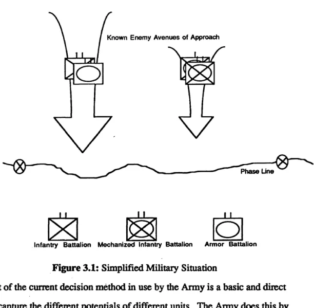
Consider a military planning staff faced with the problem of determining where to assign different units to defend against an enemy attack. The organization of each unit varies. Some units may be equipped with modem technology and may be better trained for the upcoming mission. Others may be reserve units which are incompletely manned and poorly equipped. The role of each unit on the battlefield varies, too. Some may be ground gainers such as armor and mechanized infantry. Others may deny access to terrain such as artillery, combat engineers, or aviation assets. The big picture can become very complex, very quickly. The problem is where to assign each unit to maximize friendly combat potential against the enemy. Figure 3.1 illustrates a very simple scenario using current conventional military graphics.
Known Enemy Avenues of Approach
Phase Line
i i 1i._. it
1S1
^
iqi
Infantry Battalion Mechanized Infantry Battalion Armor Battalion
Figure 3.1: Simplified Military Situation
Part of the current decision method in use by the Army is a basic and direct method to capture the different potentials of different units. The Army does this by assigning combat power indices (potentials) to each unit The indices are relative to a base unit of 1. For example, the more modem equipped American M l tank battalion may be assigned an index o f 3.5. The 3.5 means that this battalion is 3.5 times as lethal as the base unit Usually the base unit is the Soviet T-55 tank battalion assigned to an
T-4002 17
simple way of quantifying potential.
With combat power indices now assigned to both friend and foe, the staff must now determine assignments. One important assignment criterion is that of the force ratio. It is believed that the lower the ratio, the better the chance for initial success. For
example a ratio of 2 (enemy potential) over 1 (friendly potential) is better than a ratio of 4 to 1. This first example matches relatively greater friendly potential to enemy potential. So the staff analyzes different proposed alignments and determines the force ratios associated with each. It is important to note that none of the proposed alignments were formulated using the force ratio criterion. Instead the staff uses the force ratios to
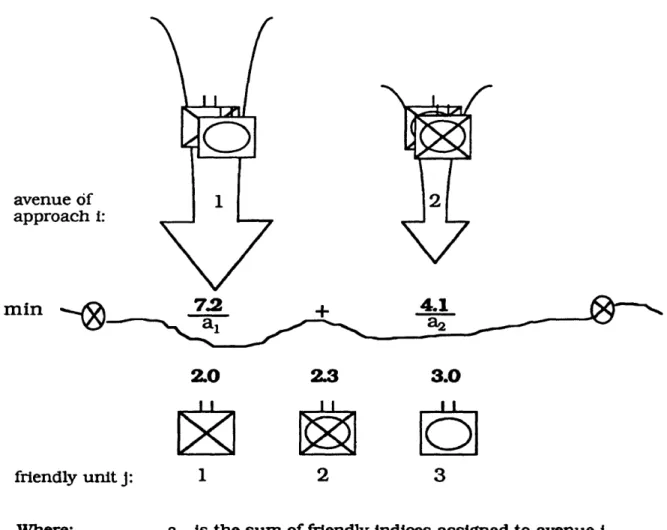
evaluate proposed options. Consequently, the option with the ratio of indices that result in the lowest fractions becomes a favored course of action by the staff. When coupled with other decision criteria such as unity of command and simplicity of execution, this course of action may gain approval by the commander for implementation. The formulation that follows recruits the force ratio criterion as an objective function. The constraints ensure that a unit is assigned in only one place and at least one unit is assigned to oppose every known enemy avenue of approach. If the enemy were unopposed, he could exploit this to his advantage. Therefore it becomes necessary to oppose every known enemy axis of advance (avenue of approach) with at least one friendly unit. This unit could be a radar unit which "listens" for activity or a combat unit which screens or engages and destroys the enemy. Figure 3.2 expands Figure 3.1 to include relevant information for the
formulation of the military problem with fractional integer programming. The combat power potentials identified in this figure will be utilized in the example of this method in Chapter 4.
avenue of approach i: m m friendly unit j: Where: 7J2 2.0 U _
[X
2.3 I i 4.1 3.0 -JJLo
1 2 3a t is the sum of friendly indices assigned to avenue i.
Subject to: Every avenue is opposed with a least one friendly unit.
Each friendly unit is assigned only once.
T-4002 19
3.2 The Integer Program Formulation
The general form of the fractional integer program can be written as follows: Minimize:
n Jr.
i = l d x
Where the denominators at are defined as:
m
for each i,
X
cpcu = a. j = i r J Subject to:m
for each i, X x{j ^ 1 ensuring at least one unit is assigned to each avenue of approach.
7 = 1 n
for each j ,
X xu = 1 ensuring that each unit is assigned exactly once.
i = 1In this formulation, each term of the objective function represents a different enemy avenue of approach. Each numerator kx represents the relative combat power of enemy units located within avenue of approach i. The denominators ax each represent the sum of relative combat power indices of friendly units that are chosen to oppose the enemy units located in avenue of approach i. The force ratio for each avenue of
approach, then, is represented by its term in the objective function. Each term should be minimized as much as possible but not at the expense of any other. The effect is that the sum of the force ratios is minimized, which is represented by the objective function.
The decision variable associates the decision to assign or not to assign friendly unit j to avenue of approach i. The constant is the enemy’s combat power index
associated with friendly unit j. The subscript i tags the decision variable to a particular avenue of approach. The subscript j tags the decision variable to a particular friendly unit.
3.3 The Integer Program Problem Solving Procedure
The steps for solving the fractional integer program are shown in a flow chart (figure 3.3). The integer programming formulation described above is illustrated in
example 1 of Chapter 4. The following problem solving technique appears to capture the objective of the military problem and uses 0-1 integer programming methodology. It should be noted that one very basic result is not proved in this thesis (see Chapter 5). This procedure relies, instead, on a conjecture. However, acceptance of this conjecture does appear to optimize the decision of which units to assign opposite which avenues so as to minimize the sum of the resulting force ratios.
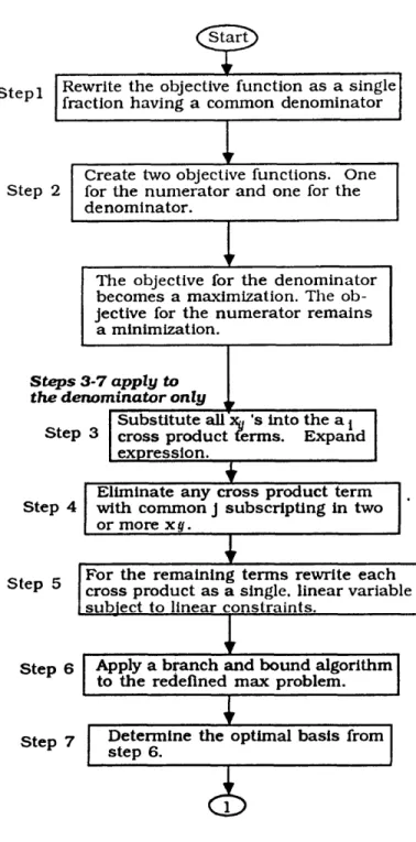
S te p l
Step
Rewrite the objective function as a single fraction having a common denom inator
Create two objective functions. One for the n u m e ra to r an d one for the denom inator.
S te p s 3-7 a p p ly to
th e denom inator only
S tep 3
Step 4
S u b stitu te all Xg's into the a j cross p ro du ct term s. Expand expression.__________________ Elim inate an y cross prod uct term w ith com mon j subscriptin g in two or m ore xg .______________________ The objective for th e denom inator becom es a maximization. The ob jective for th e n u m erato r rem ains
a minimization.
S tep 5 cross pro du ct a s a single, linear variable F or th e rem aining term s rew rite each subject to linear constraints.___________
S tep 6 Apply a b ran ch an d bound algorithm to th e redefined m ax problem.
S tep 7 D eterm ine the optim al b asis from step 6.
£
S te p s 8-11 a p p ly to ( l
th e n u m erator on ly j[
Step 8 Rewrite the numerator in exactly the sam e manner as step 3.
r
Step 9 From step 7, list the optimal basis for the m ax problem. Generate the n! different optimal bases.
r
Step 10 Construct a constraint set which limits b ases of min problem to the optimal bases o f max problem.
r
Step 11 Apply a branch and bound algorithm to the redefined min problem. Determine the optimal basis.
T-4002 23
Suppose the fractional integer objective function is:
i = i a,
Which expands to: k\ Jc2 k*
Q\ d2
STEP 1: Rewrite the objective function over a single common denominator. This gives a new objective function in the form:
^{^2^3 "I" k^Ct\CL-^ 4* k^d\d2 aid2a3
Go to step 2.
STEP 2: Create two objective functions, one for the numerator and one for the denominator of the expression from step 1. In the steps that follow, we will first
maximize the denominator, then minimize the numerator. In this example, the numerator objective becomes:
Minimize:
Similarly, the denominator objective becomes: Maximize: aia2a3
3.3.1 Maximizing the Denominator (Steps 3 thru 7):
STEP 3: Substitute all x ^ s and their coefficients into the a, cross product expressions and expand the resulting denominator into a polynomial with cross product terms only. For example suppose: Cj = 2, c2 = 3, and c3 = 4. Furthermore, suppose each a, is defined as:
d j = CjXj j + C2XI 2 + C j X 13,
0-2 = Cl X 2 l ■*" C2X 22 "*■ C3X 23>
Therefore an a, cross product expression becomes:
d j d 2 = 3 x i2 + 4 x j3) ( 2 x 21 + 3 x 22 + 4 x 2j )
Which expands to:
4xnx2I + 6xjjX22 + %xux23 + 6Xi2X21 + 9xi2*22 + 12Xiix23 + Sx13x 2} + l l x l3x22 + 1 6xJ3x23
Go to step 4.
STEP 4: Eliminate any cross product term with common j subscripting in two or m o r e l’s within the cross product The assignment constraints cause these terms to equal zero because friendly unit j can be assigned only once. In this example, the terms containing xu x21, x J2x22, and x J3x23would be eliminated. Go to step 5.
STEP 5: For the remaining terms, rewrite each decision variable cross product as a single linear variable with combined subscripting. The fact that the new variable is linear is of great importance because this limits the number of nodes that need to be searched in the branch and bound algorithm. For instance x 11x22would become x 1122.
T-4002 25
the original decision variable cross product. For each decision variable cross product introduce the following constraint sets:
For the double product let x ^ y - x^y subject to the constraints:
+ x.y - %7 < 1
xv
-% / £ 0
x,y - %7 > 0
Where the primed subscripting denotes a change in subscript values on the decision variable. Table 3.1 lists the possible values for andx,y. This table further demonstrates the consistency of values for the cross product XyXy and the new linear variable x^y subject to the above constraint set.
Table 3.1: Double Product Truth Table
Xff XijXi’f Xiji'f
1 1 1 1
1 0 0 0
0 1 0 0
0 0 0 0
For example the linear variable x1122 would be substituted for the cross product xnx22 and would then be subject to the constraints:
X11 + *22 X1122 < 1
Xu X1122 > 0
*22 X1122 > 0
In similar fashion, let the triple product = jr..., iT be si Xij + xi7 + $ S 1 *iji'j'i"j" 2
xa - > 0
xi7 - > 0
Xi-j- > 0
Go to step 6.
STEP 6: Apply a branch and bound algorithm to the redefined objective function and constraint set from step 6. Remember only the original x# s (e.g. xn) are defined as 0-1. The new variables (e.g. xU22) introduced after redefining the cross products are linear and do not need to be defined as 0-1. In this example the redefined objective function found in step 4 is:
Max 6xnx22 + $*11*23 + 6*12*21 + 12*12*23 + $*13*21 + *^*13*22 Go to step 7.
STEP 7: Determine the optimal basis for the maximization of the denominator. This optimal basis may not be the only basis that attains optimality for this objective. Indeed, a degeneracy of sorts may exist. The branch and bound algorithm will determine one optimum. However, there may be many optima which exist along parallel branches
T-4002 27
of the algorithm. It is this possibility of multiple optima (more than one set of decision variables that achieve the same maximum) that leads to the minimization of the
numerator after fixing the denominator size at its maximum. Go to step 8.
3.3.2 Minimizing the Numerator (Steps 8 thru 11):
STEP 8: In exactly the same manner as in Step 3, rewrite the numerator of the objective function. Likewise, redefine all cross products and introduce constraint sets in exactly the same manner as step 5. Go to step 9.
STEP 9: From step 7 list the denominator’s optimal basis from the branch and bound algorithm. In this step, determine all bases that are optimal for the denominator problem and constrain the numerator problem to include just one of these. This author conjectures that one of these bases is optimal for the original fractional integer program.
First it is important to remember the meaning of the ij subscripting on each x{j. The i represents the objective function term that the Xg is being assigned to (a particular avenue of approach). Whereas the j identifies the friendly unit index. It is possible to attain the same optimal value for the denominator objective with a different feasible combination of XgS equal to 1. In effect, we want to preserve the grouping of units to a particular avenue of approach. Exactly which avenue will not be known until the numerator is minimized. This can be performed by permuting the i (the avenue of approach) subscripting across the j subscripting found in the optimal basis in Step 7.
For example, suppose the optimal basis in step 7 is jcu, jc22, and x23, where each of these variables takes on the value 1. Also suppose a2 = c1x1I and a2 = c^x22 +
Consequently, the cross product, a2a2i would then equal Cifo+c^). Another optimal basis
AfiTMUfi L A O S LI® RAM r COLO&8DO 9CSSOOL ci MINES
for the maximization objective could be x21, x12 and xu. Where a1 = CjX2] and a2 = c2x12 + CjX13. The cross product, would also equal Cj(c2+c3) which is equal to the result of the first basis. In fact, it is possible to find up to n\ different optimal bases to the
maximization problem, so long as we preserve the grouping of j 's (units) in the manner discussed above. Now list the n\ different optimal bases to the denominator problem. Go to step 10.
STEP 10: This author conjectures that one of the bases in Step 9 will be optimal for the numerator problem and the original objective function. In this step, construct a constraint set of n\ + 1 different constraints and introduce n\ new variable "switches" that will activate constraints to select the appropriate optimal basis. These new
constraints and variable switches will cause one of these sets of variables to be optimal in the numerator problem. In effect, we are now combining the maximization of the
denominator and minimization of the numerator into one problem.
Let’s revisit the example in Step 9 to illustrate how this is accomplished. We want to choose either the basis jcn, x22i and x23 or x21, x12 and x13 during the minimization
objective of the numerator. The following constraints will affect this choice:
*11 +*22 + *23 - 3^1 = 0 *12 + *13 + *21 - 3 j2 = 0
yi+ yz = 1
Both yl and y2 are linear variables and do not need to be defined as 0-1. The fact that yj and y2 are linear is of great importance because this limits the number of nodes that need to be searched in the branch and bound algorithm. Go to step 11.
T-4002 29
STEP 11: Apply a branch and bound type algorithm to the redefined
minimization objective in step 8 subject to the constraint sets generated in Steps 8 and 10 and the original assignment constraints. I conjecture that the optimal basis from this numerator objective is the optimal basis for the original fractional integer programming problem. This ends the procedure.
3.4 Step-by-Step Procedure for the Near-Minimal Algorithm
The steps for establishing a near-optimal solution to the military problem are shown in a flow chart (figure 3.5). The algorithm that follows is further illustrated in example 2 in Chapter 4. The following procedure captures the objective of the military problem and uses elementary, binary mathematics such as addition and division. The worksheet in Appendix B should be used in conjunction with the procedure. The underlying principle of the algorithm is to maximize the differential between two
numbers. The first number represents the current upperbound for an objective term (the current force ratio for avenue /)• The second number represents a potentially new
upperbound for the same term should a unit be assigned there. In this way we identify the so-called "greatest bang for buck." In so doing, each iteration of the algorithm moves the objective function non-increasingly toward the minimum. Furthermore, each
iteration of the algorithm assigns a different friendly unit and corresponds to a different row of Table 1 (see figure 3.4) of the worksheet.
In each row of Table 1 columns are designated for each avenue of approach or term in the objective function. The value of box b represents the current value of the denominator of each term (at) in the objective function (See Formulation Section 3.2). The value of box c will contain the potentially new value of the denominator (^) should
the unit listed in that row be assigned there. The value of box d will contain the current force ratio for each term in the objective. The value in box e will contain the potential force ratio should the unit listed in that row be assigned there. Finally, the value of box f represents the marginal contribution for the unit listed in that row toward minimizing each of the objective function terms. When circled, the entry in box f will represent the greatest marginal contribution toward minimizing the objective. This procedure
identifies the column (avenue of approach) with the greatest entry in box f for each iteration and assigns the unit listed in that row to this column (avenue of approach). Table 2 of the worksheet records the assignments and aids in calculating the resulting force ratios. Feasibility is guaranteed through the selective incrementing of a counter in column u of Table 1. The value in box m represents the maximum feasible number of units that can be co-assigned to all avenues of approach. Any co-assignment of units to the same avenue of approach increments m. Each iteration of the algorithm compares u to m. When u becomes equal to or greater than m, then this indicates that each successive iteration must assign remaining units to avenues without a unit initially assigned. Otherwise, an avenue may be unopposed which violates tactical feasibility.
T-4002 31
Maximum number of units that can be co-asslgned Current number of units co-assigned
Enemy Combat Power Index for Avenue i
A
/
B
Row "Red" Blue
Friendly Combat Power Index for unit j Current upperbound for objective term i
Current value of denominator a t
Potentially new upperbound for objective term i Potential value of denominator a i
Marginal contribution o f unit j to objective term i
!' Figure 3.4: Exploded Worksheet Row
i
At the conclusion of this procedure, all friendly units are assigned according to Army Doctrine (a feasible solution to the military problem) and the sum of the resulting force ratios is very near the minimal value for the fractional integer program discussed earlier.
For larger problems it may be helpful to use the analogous computer program shown in Appendix E. This program is merely an automated worksheet. A tremendous time savings is the major advantage for using the program. Problems of very large size can be solved in less than half a second using the program. The manual method is possibly prone to analyst error and may take 20 or more minutes to complete for larger problems.
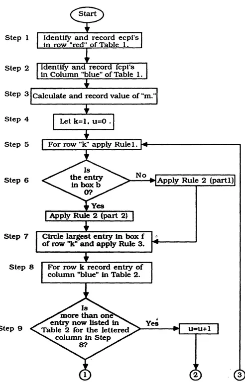
Step 1
Step 2
Step 3
Step 4
<s>
Identify and record ecpi's in row "red" of Table 1. Identify and record fcpi's in Column "blue'’ of Table 1. Calculate and record value of "m.
T ~
Let k = l. u=0 .
Step 5 | For row ”k'' apply RulelT
«*-Is Step 6
Step 7
Step 8
< C £ eut!?ikr ---- - > Apply Rule 2 (parti)
N . 0 ? /
* Y e s
| Apply Rule 2 (part 2) 1
"V '
Circle largest entry in box f o f row "k" and apply Rule 3.
For row k record entry of column "blue” in Table 2.
Step 9
more than one entry now listed in Table 2 for the lettered
column in Step
8?
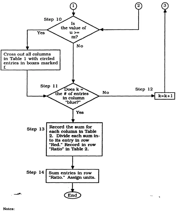
T-4002 33 Step 10 Yes No Step 11 Step 12 No Yes Step 13 Step 14 E nd >oes k The # o f entries In colum n N . "blue?" ^ the value of u >= v. m? ^ k = k + l
Sum entries in row "Ratio." Assign units.
C ross o ut all colum ns in Table 1 w ith circled en tries in boxes m arked
Record the sum for each column in Table 2. Divide each sum in to its entry in row "Red." Record in row "Ratio" in Table 2.
Notes:
Ecpl is a n abbreviation for Enemy Com bat Power Index. Fcpl is a n abbreviation for Friendly Combat Power Index.
STEP 1: Identify enemy avenues of approach. For each avenue of approach sum the enemy combat power indices* (ecpi) in the enemy’s first echelon and record each in a separate column of row "red" of Table 1. Cross out all lettered columns without entries in row "red." Enter the total number of avenues of approach in the "Total # Entries" box to the right of row "red." Go to Step 2.
♦Refer to page 3-3, CGSC ST 100-9, to obtain unclassified combat power indices for different unit types.
STEP 2: Identify friendly units available for deployment. Assign each their friendly combat power index* (fcpi). Arrange in non-increasing (decreasing) order. Record them in order in column "Blue" of Table 1. Record the number of entries in column "Blue" in the "Total # Entries" box at the bottom of Table 1. Go to Step 3. ♦Refer to page 3-3, CGSC ST 100-9, to obtain unclassified combat power indices for different unit types.
STEP 3: Subtract the value in the "Total # Entries" box to the right of row "red" from the "Total # Entries" box at bottom of column "Blue." Record in the box marked m at upper left of Table 1. Go to Step 4.
STEP 4: Let a Table 1 row counter "k" be set equal to 1. Let u=0. (Note that both counters have columns labeled in Table 1 for recording their values throughout this procedure.) Go to Step 5.
T-4002 35
RULE Is
For each used column in row k:
Add the value of column ’’Blue" to the value in box b. Record the result in box c.
Go to Step 6.
STEP 6: For row k in Table 1 apply Rule 2. Go to Step 7.
RULE 2:
For all used columns, divide the value in box c into the value in row "red". Record in box e.
//■the used column has a 0 in box b, then:
Subtract the value in box e from the value in row "red." Record result in box f.
Else, divide the value in box b into the value in row "red." Record in box d.
Subtract the value in box e from the value in box d. Record in box f.
STEP 7: For the current row (row k), circle the largest value of all boxes marked f. Apply Rule 3.
RULE 3:
For the column with the circled entry only, add the value in column "Blue" of row k to the value in box b.
Record in box b in next row (row k+1).
For all other capital lettered columns, copy the value in box b to box b of the next row (row k+1).
Go to Step 8.
STEP 8: For the current row (row k), record the value in column "Blue" to the same column of Table 2 as the entry circled in Step 7. Go to Step 9.
STEP 9: If more than one entry is now listed for the capital lettered column in Table 2 from Step 8, then u=u+l. Otherwise u is unchanged. Record this new u in column u of row k+1 of Table 1. Go to Step 10.
STEP 10: Is the value of u ^ m? If so, cross out all capital lettered columns in Table 1 with circled entries in boxes marked f. No further calculations are necessary for these columns. Go to Step 11.
STEP 11: Is the number of rows filled in equal to the number of entries in column "Blue?" If no, go to Step 12. If yes, go to Step 13.
T-4002 37
STEP 13: For each capital lettered column of Table 2 sum its entries and record in row "total" in Table 2. Divide this sum into the value in row "Red" of Table 1. Record the result in row "Ratio" of Table 2. Go to Step 14.
STEP 14: Sum all entries in row "Ratio" of Table 2. This sum is the near minimal value for the force ratio problem. Assign units with the combat power indices listed in Table 2 to the Avenue of Approach corresponding to the lettered column they are listed. This ends the procedure.
Chapter 4
EXAMPLE PROBLEMS
This chapter illustrates both the fractional integer programming procedure and the near-minimal algorithm with several examples. The first example is a fractional integer program of meager size. However, notice the length and complexity of the problem solving. All successive examples illuminate the near-minimal algorithm.
4.1 Example 1 (Using Fractional Integer Programming) 4.1.1 Problem Statement
Minimize the force ratios between 3 friendly units with combat power indices of 3,2.3, and 2 and enemy units assigned along 2 avenues of approach with combat power indices of 7.2 and 4.1. Figures 3.1 and 3.2 graphically illustrate this first example.
4.1.2 Fractional Integer Program Formulation
The fractional integer formulation was discussed in detail in Chapter 3. This method will serve to choose the units for each avenue of approach to minimize the expression below which, in effect, minimizes the sum of ratios of the enemy’s combat power indices to the units chosen to oppose it there. The fractional programming problem which formulates the example above would look like the following:
T-4002 39
Minimize: 7I2 + 4I1
d\ O2
Let = 1, if along avenue of approach i, friendly unit j is assigned. Otherwise - 0.
Where: a\ - 3*n + 2.3jc12 + 2x13 — 3^21 "t" 2 .3 * 2 2 2*23 subject to: * 1 1 + *1 2 + * 1 3 *11 + *21 = 1 *12 + *22 = 1 * 1 3 + * 2 3 = 1
4.1.3 Integer Programming Problem Solving Procedure:
STEP 1: By combining the objective function terms into a single fraction, the objective function becomes:
min 7.202 + 4.10! (4.1)
STEPS 2-3: From chapter 3, it was conjectured that the minimum of eq. 4.1 will exist at a maximum of axa2, Expanding this expression yields:
Max axa2 =
9*n*2i + 6 .9 x 12x21 + 6 x 13x21 + 6.9xnx22 + 5.29x12x22 + 4.6x13x22 + 6xnx23 + 4.6x12x23 + 4x13x23
STEP 4: Since all jc./s are either 0 or 1 and subject to the assignment constraints above, some terms can be eliminated which will equal 0 at feasibility. The Maximization problem now becomes:
Max axa2 = 6.9xX2x2X + 6xX3x2X + 6.9xux22+ 4.6x13x22+ 6xnx23 + 4.6xl2x23
STEP 5: Next it will be necessary to redefine each cross product in the objective function as a new variable subject to additional linear constraints.
Let XijXiy = X w
Subject to the additional constraints: xtJ + xi y - x ili7 <, 1
Xy - Xyjy — 0 Xi-r - xijt-r > 0
For this problem the above constraint types are formulated below:
* 7 2 + * 2 7 *7227 < = 1 * 7 2 -*7227 > = 0 * 2 7 *7227 > = 0 * 7 3 + * 2 7 -*7327 < = 1 X 13 -*7327 > = 0 * 2 7 -*7327 > = 0 + * 2 2 *7722 < = 1
T-4002 41 Xu X U 22 >=0 + X 22 X U 22 >=0 X l 3 + x 22 X 1322 <=1 X j 3 X 1322 >=0 X 22 X j3 2 2 >=0 Xu + X 23 - X U 23 <=1 Xu - X U 23 >=0 X 23 - X U 23 >=0 X i2 + X 23 - X 1223 <=1 X J2 -X J223 >=0 X 23 -X 1223 >=0
STEP 6: Apply a branch and bound algorithm to this objective function and constraints.
STEP 7: The optimal basis is: {xu, x22* x23).
STEP 8: Examining the numerator as the minimization problem we have: Min 7.2fl2 + 4. la u
Expanding this expression after substituting the appropriate *,/s for a} and a2 we have: Min 21.6*2! +16.56*22 +14.4*23 + 12.3*n + 9.43*12 + 8.2*13
STEP 9: We can generate n\ different solution sets which yield the same value for the objective function. In this example n (section 3.2), the number of avenues of approach, is 2. This degeneracy of sorts is caused by the x{j sums in the expressions a1
and a2. Subject to the above constraints, each of these expressions can actually take on n different combinations of these 0-1 variables in which the coefficients of the variables equal to 1 maximize the expression a ^ . Figure 4.1 illustrates the two bases which maximize the denominator expression found in eq. 4.1. The other optimal solution to the maximization objective is [x12, x13, x21). The minimization of the original objective function will be the intersection between the solution space for the numerator and
denominator objectives. The information about the maximization function will now constrain the minimization function to just these choices of decision variables. We can now write additional constraints which will cause one and only one of these sets of variables to be basic in the minimization objective. The numerator minimization objective, properly constrained, will become the minimum for the original objective.
T-4002 43 avenue of approach i: W h ic h i s m in ? 7.2 4.1 7 .2(2.0) + 4 .1 (2.3+3.0) 2.0(2.3+3.0) 7 .2(2.3+ 3.0) + 4 .1 (2 . (2.3+3.0)2.0 2.0 I I friendly unit j: 2 3 I 3 .0
o
STEP 10: Three (nl + 1) new constraints would restrict the minimization solution space to one of the maximization solutions. These constraints are:
Xjj +x22'*~x23~3yi =0
x12+xI3+x2i -3y2=0
y i + y2= i
The coefficient, 3, on y2 and y2 in the first two constraints causes yt and y2 to equal either 0 or 1 depending on which set of *^s are basic. Earlier it was stated either *iis x22, and x23 all equal 1 or x12, x13, and*2/ all equal 1. Both sets of *yS cannot be chosen because the third constraint causes either y7 ory2 to equal 1. Thus the yt acts as a "switch" by activating the decision variables contained in one the first two constraints to equal 1 at feasibility.
STEP 11: The redefined minimization problem becomes: Min 21.6*2! + 16.56*22 +14.4*23 + 12.3*n + 9.43*12 + 8.2*13 Subject to: *H +*12+ *i3 *2i + * 2 2 + X 23 *U + *21 * 1 2 + * 2 2 *13 + *23 > = 1 > = 1 = 1 = 1 = 1
T-4002 45
Additionally, from the maximization of the denominator problem:
x,i ' + x22 + x23 - 3y, = 0 xl2 + xl3 + x2l -3y2 = 0
y2 + y2 = 1
Now using a branch and bound minimization method, the above 0-1 formulation yields the following solution: The optimal basis is {x12, x13, x21}. These variables yield a minimum objective value of 3.04 to the original objective function:
T2 + 4JL
Cl\ d 2
4.1.4 Conclusions
Even though this problem is small, the procedure is lengthy. In fact there are only six feasible solutions to this problem. To illustrate the growing complexity of this
formulation, examine a slightly larger problem. Consider assigning five units opposite just three avenues of approach. Table 4.1 lists the types and numbers of constraints and variables generated in this kind of formulation.