Progress in stochastic analysis, modeling, and simulation: SAMS-2003

Full text

(1)Hydrology Days 2003, 165-175. Progress in Stochastic Analysis, Modeling, and Simulation: SAMS-2003 O.G. B. Sveinsson1, J.D. Salas2, W.L. Lane3, and D.K. Frevert4 1. Post-Doctoral Fellow, International Research Institute (IRI), Columbia University, N. York (formerly graduate student at Colorado State University, Fort Collins, Colorado). 2 Professor of Civil Engineering, Colorado State University, Fort Collins, Colorado 80523 (on sabbatical leave at the Institute of Hydromechanics and Water Resources Management, ETH, Zurich, Switzerland) 3 Private Consultant, Golden, Colorado 80401 (formerly at the U.S. Bureau of Reclamation, Denver, Colorado). 4 Hydraulic Engineer, U.S. Bureau of Reclamation, Technical Services Center, Lakewood, Colorado 80225 Abstract. SAMS is a software for stochastic analysis, modeling, and simulation of hydrologic time series such as streamflows. It has been written in MS Visual C++ and Fortran. The package consists of many menu option windows that focus on three primary application modules - Statistical Analysis of Data, Fitting of a Stochastic Model (including parameter estimation and testing), and Generating Synthetic Series. SAMS has the capability of analyzing single site and multisite annual and seasonal data such as monthly and weekly streamflows based on a number of single site and multisite models, and aggregation and disaggregation modeling schemes. Results can be presented in graphical and tabular forms and, if desired, saved to an output file. The purpose of the paper is to summarize and update on the current capabilities of SAMS. Some illustrations are made to demonstrate the improved technical capabilities of the program using flow data of the Colorado River system.. 1. Introduction Stochastic hydrology has been a technology available to many water organizations for several decades. For instance, the U.S. Army Corps of Engineers (USACE, 1971) developed the HEC-4 model which has been widely used for extension and generation of monthly hydrologic data such as streamflows. Likewise, the U.S. Bureau of Reclamation developed the LAST (Lane Applied Stochastic Techniques) stochastic hydrology package in the late 1970’s for the purpose of modeling and simulation of streamflows for multi-site stream network systems (Lane, 1978; Lane and Frevert, 1990). Typical applications of stochastic analysis and simulation include reservoir capacity determination, reservoir yield analysis, low flow and drought analysis, evaluating operating rules of reservoir systems, performance evaluation of hydraulic structures under uncertain streamflows, irrigation system evaluation under uncertain water deliveries, and water resources impact analysis of climate change (Salas et al, 1980; Loucks et al, 1981; Salas, 1993; Hipel and McLeod, 1994). Despite of the availability of general-purpose statistical software such as S-Plus, SAS/ETS, SPSS, MINITAB, STATVIEW, IMSL, and MATLAB, etc., specialized software for frequency analysis of extreme hydrologic events such as extreme precipitation and extreme floods, and software for simulation of hydrologic time series such as annual and monthly streamflows, have been attractive in the field because of several reasons (Salas et al, 2003). Firstly,  Hydrology Days 2003.

(2) Sveinsson et al.. hydrologic time series may require stochastic models that may not be readily available in standard statistical packages such as models with long memory, and models that may be capable of producing shifting patterns such as those that are observed in certain hydrometeorological processes. Secondly, the periodic nature of hydrological processes, such as monthly and weekly streamflows, require periodic stochastic models or models with periodically varying parameters. Lastly, many of the stochastic models and simulation schemes that are useful for complex hydrologic and water resources systems, such as models for temporal and spatial disaggregation, have been developed specifically to fit the needs of water resources. In addition to HEC-4 and LAST as noted above, SPIGOT (Grygier and Stedinger, 1990) and more recently, SAMS (Salas et al, 2002) are specific software packages developed for multisite hydrologic simulation. The latter software SAMS, which stands for Stochastic Analysis, Modeling and Simulation, has been developed in collaboration between Colorado State University and the U.S. Bureau of Reclamation (Salas et al, 2003). The main purpose of this paper is to summarize the capabilities of SAMS2003 and to illustrate some of them by using a case study. First, a brief summary of the key concepts utilized in stochastic simulation is made followed by another section that summarizes the current features of SAMS-2003. Subsequently, some of the capabilities of SAMS are illustrated using data of the Colorado River System.. 2. Stochastic Simulation Stochastic simulation of hydrologic time series is generally conducted using mathematical models. These models commonly require analyzing the temporal and spatial variability of the series under consideration. For example, first and second order statistics such as the mean, variance, and covariance are useful in any type of statistical analysis. Higher order moments such as skewness, and some other statistics related to surplus, drought, and storage are of interest from the practical standpoint. Furthermore, most of the stochastic models available for simulation assume that the underlying variable is normally distributed, an assumption that is not generally met by most hydrologic data. Thus it is commonly necessary to test the hypothesis that the original data are normally distributed and to transform them into normal if the hypothesis is rejected. A number of stochastic models have been suggested in literature for stochastic simulation of hydrologic processes such as streamflow (e.g. Salas, 1993; Hipel and McLeod, 1994). One of the most popular and simplest models is the autoregressive model denoted as AR(p) as shown in Table 1. This model has been widely utilized for stochastic simulation of hydrologic and water resources data. Choosing a type of model for the data at hand depends on several factors such as, physical and statistical features of the process under consideration, complexity of the system, purpose of the study, experience, and often the availability of specialized software (Salas et al, 1980). Furthermore, for complex water resources systems, “modeling schemes”, which are  Hydrology Days 2003. 166.

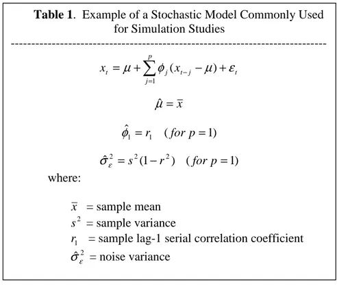
(3) Progress in Stochastic Analysis, Modeling and Simulation. assembly of several models linked in certain ways depending on the system’s configuration, the number of sites, and the objective of the study is generally needed (Salas et al, 1980; Grygier and Stedinger, 1990). Once the stochastic model and modeling scheme have been defined for the system at hand, the next step is to estimate the model parameters. This can be accomplished based on the method of moments or maximum likelihood depending on the model and modeling scheme. The model(s) are then tested using certain goodness of fit and evaluation criteria to judge whether they comply with the underlying assumptions of the model and whether they are capable of producing statistical features and hydrologic events that are important for the problem at hand (e.g. Salas et al., 1980; Loucks et al, 1981; Salas, 1993; Hipel and MacLeod, 1994). Finally, based on the selected stochastic model, simulations (data generation) are performed for the intended objective (e.g. evaluating the performance of a reservoir built for supplying supplemental water to an irrigation system). Figure 1 briefly summarizes the various steps as noted above.. Table 1. Example of a Stochastic Model Commonly Used for Simulation Studies ----------------------------------------------------------------------------p. xt = µ + ∑ φ j ( x t − j − µ ) + ε t j =1. µˆ = x. φˆ1 = r1 ( for p = 1) σˆ ε2 = s 2 (1 − r 2 ) ( for p = 1) where: x = sample mean s 2 = sample variance r1 = sample lag-1 serial correlation coefficient σˆ ε2 = noise variance. 3. Capabilities of SAMS-2003 SAMS-2003 has been written in C++ and Fortran and runs under modern windows operating systems such as WINDOWS 2000. Its menu allows the user to choose between numerous analytical options, particularly (a) Stochastic Analysis of Data, (b) Fitting a Stochastic Model, and (c) Generating Synthetic Series. Some key features of SAMS-2003 are summarized in Table 2. A key concept in SAMS is that of temporal and spatial disaggregation (downscaling). Spatial disaggregation relies on the concept of key stations,  Hydrology Days 2003. 167.

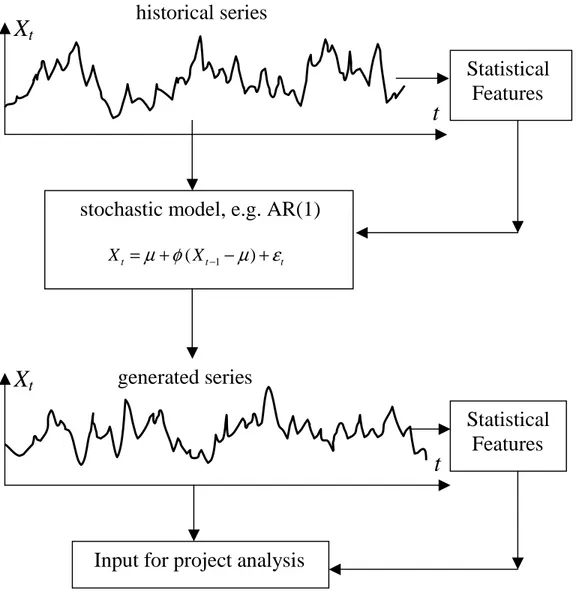
(4) Sveinsson et al.. substations, subsequent stations, and further “upstream” stations. In some cases, the key stations may be the farthest downstream stations, substations are the next stations upstream, subsequent stations are next further upstream stations, and so on. SAMS has the capability of unlimited sequence of stations. Three schemes are available for modeling the data of the key stations and upstream stations as summarized in Table 2. In Schemes 1 and 2 annual generation is conducted first, and subsequently the annual quantities are temporally disaggregated into seasonal. In Scheme 3 seasonal quantities are first. Xt. historical series. t. Statistical Features. stochastic model, e.g. AR(1) X t = µ + φ ( X t −1 − µ ) + ε t. Xt. generated series. t. Statistical Features. Input for project analysis. Figure 1. Schematic of stochastic generation using an AR(1) model built from the historical series. Simulations are performed that provide a wide range of possible flow traces that may occur in the future. They also useful for testing project design and management alternatives..  Hydrology Days 2003. 168.

(5) Progress in Stochastic Analysis, Modeling and Simulation. Table 2. Main features currently available in SAMS-2003 Main Functions Stochastic Analysis. Stochastic Modeling. Temporal Scale Annual. Seasonal Sub-seasonal (e.g. weekly) Daily Annual. Seasonal. Features • Basic 1st and 2nd order statistics and skewness • Drought related statistics • Surplus related statistics • Storage related statistics • Data transformations Same as above Same as above Same as above Single site: AR(p), ARMA(p,q), GAR(1), SM* Multisite: MAR, CARMA, CSM*, CSM-CARMA* Spatial disaggregation: VS, MR Single site: PAR(p), PARMA(p,q) Multisite: MPAR(p) Scheme 1: - Univariate generation, annual at index-station - Spatial disaggregation, annual at index station to annual at key stations - Multivariate disaggregation, annual at key stations to annual at substations - Multivariate disaggregation, annual at substations to annual at further upstream stations, etc. - Multivariate disaggregation of annual to seasonal at any group of stations Scheme 2: - Multivariate generation, annual at key stations - Then the same steps as above Scheme 3*: (Grygier-Stedinger’s method) - Multivariate generation, annual at key stations - Multivariate disaggregation, annual to seasonal at key stations - Multivariate spatial disaggregation, seasonal at key stations to seasonal at substations - Multivariate spatial disaggregation, seasonal at substations to further upstream stations. Not currently available except in one step.. Sub-seasonal (e.g. weekly) Daily Not currently available Stochastic Annual Available for any models/schemes as specified above Simulation Seasonal Available for any models/schemes as specified above Sub-seasonal Not currently available (e.g. weekly) Daily Not currently available * To become available by June 2003.  Hydrology Days 2003. 169.

(6) Sveinsson et al.. generated at key stations, then they are spatially disaggregated (into seasonal quantities) at other upstream stations. If seasonal data (e.g. monthly) are desired in Schemes 1 and 2, temporal disaggregation models are fitted to disaggregate the annual values at desired stations into seasonal values. Seasonal time scales may be monthly, weekly, quarter-monthly or any desired partitions of the calendar year. Current temporal disaggregation models are not recommended for use with time periods shorter than weekly. In the near future, plans are in place for the addition of models appropriate for a second level of temporal disaggregation that will allow the generation of sub-seasonal quantities (e.g. quarter-monthly or weekly after a previous temporal disaggregation from annual to monthly) or daily values. Furthermore, spatial and temporal disaggregation models can be fitted to all stations at once (one group containing all the stations) or to stations arranged in various groups. In summary, SAMS-2003 statistically analyzes and transforms the input data as needed, fits models based on any of the various options available, and generates synthetic hydrologic data. The statistical characteristics of the observed and generated data and the generated samples are presented in graphical or tabular forms and printed or written on special output files and they can be copied into Excel.. Case Example A brief illustration is presented herein to demonstrate some of the capabilities of SAMS 2003 using the data of the Upper Colorado River system. Stochastic data bases had been generated for the Colorado in the 1980’s using the LAST program (Lane and Frevert, 1990). The Colorado River is one of the important river systems of the United States and one of the most important sources of water supply for seven western states including Colorado, Wyoming, Utah, New Mexico, Arizona, Nevada, and California. Its basin includes parts of these seven states and the Republic of Mexico. The waters of the Colorado are utilized for irrigation, municipal, hydropower, industrial, mining, recreational and environmental purposes. The Colorado River system has been subject to a number of adverse climatic episodes ranging from wet periods to periods of drought (US Bureau of Reclamation, 1986 and Fulp and Harkins, 2001). Historically observed streamflow data show periods of high flows such as those that formed the basis of the 1922 Colorado River Compact and also the very high flow years of 1982-83 and 1983-84. On the other hand, the record also shows periods of drought such as the dust bowl years of the late 1920s and 1930s and also the mid 1950s. While the current state of the art does not allow accurate long-range prediction of these climatic extremes, the stochastic approach to hydrologic data can offer managers a better understanding and appreciation of the types of streamflow extremes they may face in the future. For this example, we utilized 85 years of historically observed monthly data at 16 sites in the basin (Fig.2). Prior to using SAMS, the data at some sites have been extended in order to make them cover the same period at all sites. Likewise, the data have been “naturalized” in order to remove from the measured flow data the effect of regulation or diversions. We analyzed both  Hydrology Days 2003. 170.

(7) Progress in Stochastic Analysis, Modeling and Simulation. Figure 2. Schematic of the streamflow network for 16 sites of the Upper Colorado River System.. the annual and the monthly streamflow series. Figure 3 shows the table of the input file monthly data for the 16 sites. SAMS has been used to determine basic annual statistics (mean, standard deviation, skewness, auto-correlations and cross-correlations) as well as storage and drought related statistics in both the original and transformed (into normally distributed flows) domains. Also for the monthly series monthly statistics have been determined such as, monthly means, standard deviations, skewness coefficients, and month-tomonth correlations and cross-correlations. For illustration Fig. 4 shows the correlogram of the annual flows for site 16 while Fig. 5 shows the month-tomonth cross-correlations for sites 8 and 16. Figure 6 illustrates the results obtained for transforming the June flows (season 6) for site 16 using a logarithmic transformation. It shows the distribution of annual flows in the original and lognormal domains using a normal probability paper.. Figure 3. Input file of the monthly streamflow data for the 16-site network.  Hydrology Days 2003. 171.

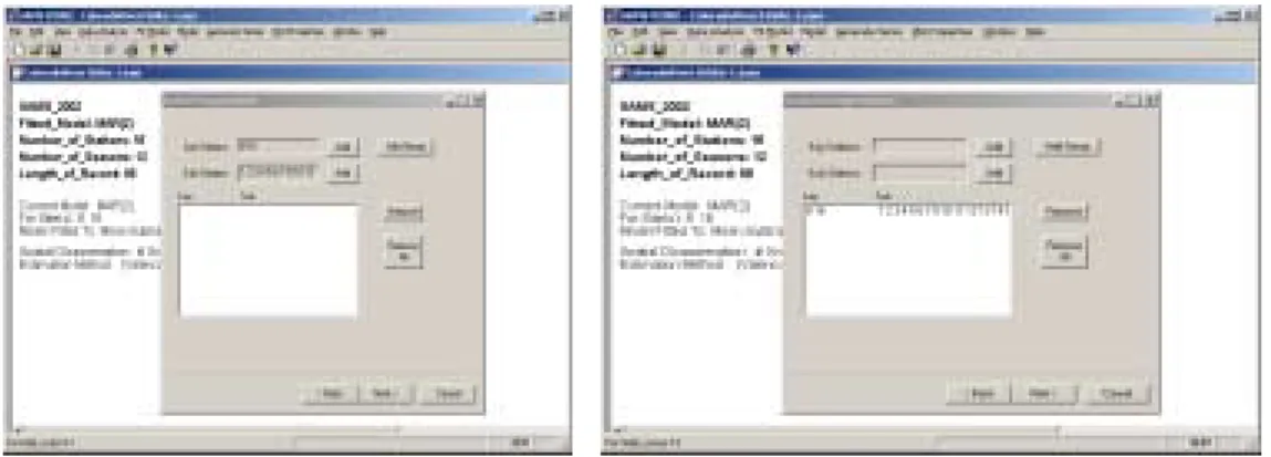
(8) Sveinsson et al.. Figure 4. Correlogram of the annual flows for site 16.. Figure 6. Distribution of June flows for site 16 using logarithmic transformation.. Figure 5. Month-to-month crosscorrelations for sites 8 and 16.. Figure 7. ARMA(1,0) parameters for the annual log-transformed flows for site 16.. Figure 7 displays results of fitting the ARMA(1,0) model to the annual log-transformed flows for site 16. The mean and the variance (i.e. x = 408.8, s 2 = 7133.3 ) of the underlying log-transformed annual flows and the model parameters: φˆ = 0.256 and σˆ 2 = 6666.7 are shown. Figure 8 disε. 1. plays a table of results comparing some historical and generated statistics using the referred AR(1) model. The generated statistics are actually the average of the statistics obtained from a specified number of simulated samples. Then, Fig.9 is a comparison of the historical sample and a generated sample of the same length as the historical. Figures 10-14 illustrate the case in which 16 stations (1 through 16) were utilized for modeling the monthly flows of the 16-site system. We selected the modeling scheme 2 as shown in Fig.10. This figure also shows that the Valencia-Schaake model was selected for the spatial disaggregation. Figure 11 shows the window menu where stations 8 and 16 are selected as the key stations and the MAR(2) (multivariate autoregressive model of order 2) model is used for fitting both sites jointly. Fig. 12 shows that sites 1, 2, 3, 4, 5, 6, 7, 9, 10, 11, 12, 13, 14, 15 (actually the last three number are not shown in the figure) will be the substations that correspond to  Hydrology Days 2003. 172.

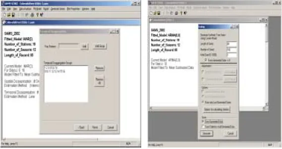
(9) Progress in Stochastic Analysis, Modeling and Simulation. the key sites 8 and 16. They are put together into a single group for fitting a spatial disaggregation model to disaggregate the annual flows of sites 8 and 16 into the annual flows for the other 14 sites as Fig. 13 shows. Then Fig. 14 shows that two groups of stations (1, 2, 3, 4, 5, 6, 7, 8) and (9, 10, 11, 12, 13, 14, 15, 16) were selected for the temporal model, i.e. to disaggregate the annual flows into the monthly flows.. Figure 8. Comparison of historical and gene- Figure 9. Comparison of historical and generated basic statistics for annual flows (site 16) rated annual flows for site 16.. Figure 10. Window menu for selecting a Figure 11. Sites 8 and 16 are the selected key modeling scheme and spatial disaggregation. sites and MAR(2) model is the chosen model.. Figure 9. rrr. Figure 10. nnn. Figure 12. Selection of substations belong- Figure 13. The key sites 8 and 16 and the subging to sites 8 and 16. stations 1, 2, 3, etc. are put into one group..  Hydrology Days 2003. 173.

(10) Sveinsson et al.. Finally, Fig. 15 shows the window menu utilized for selecting options for data generation. The generation is performed based on the model specification (including data transformations and standardizations as the case may be) determined previously. For illustration the model is ARMA(0,0) for site 16, the length of the generated series is 85 years, and the number of samples to generate is 100. In addition, the menu indicates that the generated data will be saved (on a file). Data generated by SAMS on the Colorado River is being utilized in long term studies of the Colorado for both Bureau of Reclamation and its clients. These studies required development of a set of data management interfaces between SAMS and the RiverWare modeling framework developed by the Center for Advanced Decision Support for Water and Environmental Systems (CADSWES) at the University of Colorado (Zagona, et al, 2001) and the Hydrologic Data Base used by Reclamation for management of the Colorado River basin. Results of such analysis integrating both modeling frameworks will be described elsewhere.. Figure 14. Temporal disaggregation will be made for the two groups of stations as shown.. Figure 15. Windows menu for selection of options for data generation.. Acknowledgments. The effort reported in this paper has been financed, in large part by the Science and Technology Program of the U.S. Bureau of Reclamation, with in kind services from Colorado State University (CSU), the Bureau of Reclamation’s Lower Colorado Regional Office and Technical Service Center, the Bonneville Power Administration, the Great Lakes Environmental Research Laboratory, NOAA, and HydroQuebec, Canada. SAMS was developed under the direction of J.D. Salas, W. Lane and D. Frevert with substantial contributions to the capabilities of SAMS- 2000 made by former CSU graduate students, namely: M. AbdelMohsen, N. Saada, and C. Chung. The new version SAMS-2003 has been developed building upon the previous SAMS- 2000 but with substantial changes and re-structuring made by O.G.B.  Hydrology Days 2003. 174.

(11) Progress in Stochastic Analysis, Modeling and Simulation. Sveinsson, also a former CSU graduate student. The technical effort to utilize the stochastic data base in RiverWare on the Colorado River Basin has been strongly supported by Dr. T. Fulp of the Bureau of Reclamation’s Lower Colorado Regional Office, by Mr. D. King of the Bureau of Reclamation’s Technical Service Center and by Dr. E. Zagona and Mr. J. Prairie of the University of Colorado’s Center for Advanced Decision Support for Water and Environmental Systems (CADSWES).. References Fulp, T and J. Harkins, 2001: Policy Analysis Using RiverWare. Colorado River Interim Surplus Guidelines. Bridging the Gap: Meeting the World’s Water and Environmental Resources Challenges, Proceedings of the Conference of the American Society of Civil Engineers. Grygier, J.C., and J.R. Stedinger, 1990: SPIGOT, A Synthetic Streamflow Generation Software Package. Technical description, version 2.5, School of Civil and Environmental Engineering, Cornell University, Ithaca, N.Y. Hipel, K.W. and A.I. McLeod, 1994: Time Series Modeling of Water Resources and Environmental Systems. Developments in Water Science 45, Elsevier, Amsterdam. Lane, W.L., 1978: Applied Stochastic Techniques (LAST computer package). User’s manual, Division of Planning Technical Services, Bureau of Reclamation, Denver, Colorado. Lane W.L. and D.K. Frevert, 1990: Applied Stochastic Techniques. Personal Computer Version 5.2, User's Manual”, Earth Sciences Division, U.S. Bureau of Reclamation, Denver, Colorado. Loucks, P., J.R. Stedinger, and D.A. Haith, 1981: Water Resources Systems Planning and Analysis, Prentice-Hall, Englewood Cliffs, New Jersey. Salas, J.D., J. Delleur, V. Yevjevich, and W. Lane, 1980: Applied Modeling of Hydrologic Time Series. Water Resources Publications, Littleton, Colorado. Salas, J.D., 1993: Analysis and Modeling of Hydrologic Time Series. In Handbook of Hydrology, D.R. Maidment Editor, McGraw Hill Inc., New York. Salas, J.D., O.G. Sveinsson, W.L. Lane and D.K. Frevert, 2003: Stochastic Streamflow Simulation Using SAMS 2002. Submitted to the ASCE Journal of Irrigation and Drainage. USACE (U.S. Army Corps of Engineers), 1971: HEC-4 Monthly Streamflow Simulation. Hydrologic Engineering Center, Davis, California. US Bureau of Reclamation, 1986: Executive Summary, Colorado River Alternative Operating Strategies for Distributing Surplus Water and Avoiding Spills. Zagona, E.A., T.J Fulp, R. Shane, T. Magee, and H.M. Goranflo, 2001: RiverWare: A Generalized Tool for Complex Reservoir Systems Modeling. Journal of the American Water Resources Association, Volume 37, Number 4, Middleburg, Virginia..  Hydrology Days 2003. 175.

(12)

No results found