www.atmos-chem-phys.net/11/5431/2011/ doi:10.5194/acp-11-5431-2011
© Author(s) 2011. CC Attribution 3.0 License.
Chemistry
and Physics
Aerosol indirect effects in a multi-scale aerosol-climate model
PNNL-MMF
M. Wang1, S. Ghan1, M. Ovchinnikov1, X. Liu1, R. Easter1, E. Kassianov1, Y. Qian1, and H. Morrison2
1Atmospheric Science and Global Change Division, Pacific Northwest National Laboratory, Richland, Washington, USA 2Mesoscale and Microscale Meteorology Division, National Center for Atmospheric Research, Boulder, Colorado, USA
Received: 14 January 2011 – Published in Atmos. Chem. Phys. Discuss.: 31 January 2011 Revised: 30 May 2011 – Accepted: 30 May 2011 – Published: 9 June 2011
Abstract. Much of the large uncertainty in estimates of
an-thropogenic aerosol effects on climate arises from the multi-scale nature of the interactions between aerosols, clouds and dynamics, which are difficult to represent in conventional general circulation models (GCMs). In this study, we use a multi-scale aerosol-climate model that treats aerosols and clouds across multiple scales to study aerosol indirect effects. This multi-scale aerosol-climate model is an extension of a multi-scale modeling framework (MMF) model that embeds a cloud-resolving model (CRM) within each vertical column of a GCM grid. The extension allows a more physically-based treatment of aerosol-cloud interactions in both strat-iform and convective clouds on the global scale in a com-putationally feasible way. Simulated model fields, includ-ing liquid water path (LWP), ice water path, cloud fraction, shortwave and longwave cloud forcing, precipitation, water vapor, and cloud droplet number concentration are in rea-sonable agreement with observations. The new model per-forms quantitatively similar to the previous version of the MMF model in terms of simulated cloud fraction and pre-cipitation. The simulated change in shortwave cloud forc-ing from anthropogenic aerosols is −0.77 W m−2, which is less than half of that (−1.79 W m−2)calculated by the host GCM (NCAR CAM5) with traditional cloud parameteriza-tions and is also at the low end of the estimates of other con-ventional global aerosol-climate models. The smaller forc-ing in the MMF model is attributed to a smaller (3.9 %) in-crease in LWP from preindustrial conditions (PI) to present day (PD) compared with 15.6 % increase in LWP in strati-form clouds in CAM5. The difference is caused by a much smaller response in LWP to a given perturbation in cloud condensation nuclei (CCN) concentrations from PI to PD in the MMF (about one-third of that in CAM5), and, to a lesser
Correspondence to: M. Wang
(minghuai.wang@pnnl.gov)
extent, by a smaller relative increase in CCN concentrations from PI to PD in the MMF (about 26 % smaller than that in CAM5). The smaller relative increase in CCN concen-trations in the MMF is caused in part by a smaller increase in aerosol lifetime from PI to PD in the MMF, a positive feedback in aerosol indirect effects induced by cloud life-time effects from aerosols. The smaller response in LWP to anthropogenic aerosols in the MMF model is consistent with observations and with high resolution model studies, which may indicate that aerosol indirect effects simulated in conventional global climate models are overestimated and point to the need to use global high resolution models, such as MMF models or global CRMs, to study aerosol indirect effects. The simulated total anthropogenic aerosol effect in the MMF is −1.05 W m−2, which is close to the Murphy et
al. (2009) inverse estimate of −1.1 ± 0.4 W m−2(1σ ) based
on the examination of the Earth’s energy balance. Further improvements in the representation of ice nucleation and low clouds in MMF are needed to refine the aerosol indirect ef-fect estimate.
1 Introduction
Clouds are an extremely important climate regulator. They have a large impact on the Earth’s energy budget and play a central role in the hydrological cycle. By acting as cloud condensation nuclei (CCN) or ice nuclei (IN), anthro-pogenic aerosols can modify cloud optical and physical prop-erties, and therefore affect the climate system, giving rise to the so-called aerosol indirect effect. Uncertainties in esti-mates of the anthropogenic aerosol indirect effect still dom-inate uncertainties in the estimates of radiative forcing of past and future climate change, despite more than a decade of effort on this issue (Forster et al., 2007; IPCC, 2007; Lohmann et al., 2010).
Much of this uncertainty arises from the multi-scale na-ture of the interactions between aerosols, clouds, and dynam-ics (e.g., Rosenfeld et al., 2006; Wood et al., 2011). These interactions span a wide range in spatial scales, from 0.01– 10 µm for droplet and crystal nucleation, to 10–1000 m for turbulence-driven updrafts, to 2–10 km for deep convection, to 50–100 km for large-scale cloud systems. Given the typi-cal general circulation model (GCM) grid spacing of a hun-dred kilometers, the treatment of most of those processes is highly parameterized in conventional GCMs and therefore may not be accurate.
One example is cloud lifetime effects from aerosols. In most GCMs, it is assumed that, because of less efficient coalescence and collection among cloud droplets, increas-ing cloud droplet number concentrations from anthropogenic aerosols always slow formation of precipitation and increases liquid water path (LWP) and cloud lifetime (Albrecht, 1989). However, observations show evidence of both decreasing and increasing LWP with increasing aerosols (Platnick et al., 2000; Coakley and Walsh, 2002; Kaufman et al., 2005; Matsui et al., 2006), and cloud resolving model (CRM) studies show that changes in LWP depend on meteorolog-ical conditions (Ackerman et al., 2004; Xue et al., 2008; Small et al., 2009).
It is even more problematic to represent aerosol/cloud pro-cesses in deep cumulus clouds in GCMs. Cumulus parame-terizations in current climate models rely on ad hoc closure assumptions designed to diagnose the latent heating and ver-tical transport of heat and moisture by deep convection, and provide little information about microphysics or updraft ve-locity (Emanuel and Zivkovic-Rothman, 1999; Del Genio et al., 2005; Zhang et al., 2005). As a result, only a handful of GCMs have treated aerosol effects on convective clouds in their estimates of aerosol indirect effects (Menon and Rot-stayn, 2006; Lohmann, 2008), and because those treatments were based on conventional cumulus parameterizations, the treatments are quite crude. Menon and Rotstayn (2006) in-troduced a physically-based treatment of aerosol effects on convective cloud microphysics in two GCMs and found a strong dependence of indirect effects on the details of the cu-mulus parameterization: including aerosol effects on convec-tive clouds increased aerosol indirect effects in one GCM but slightly decreased aerosol indirect effects in the other GCM. Lohmann (2008) investigated aerosol effects on convective clouds by extending a double-moment cloud microphysics scheme developed for stratiform clouds to convective clouds, and found that including aerosol effects in convective clouds reduces the sensitivity of the LWP to aerosol optical depth (AOD), which is in better agreement with observations and large-eddy simulation studies and leads to slightly smaller to-tal aerosol forcing. Clearly, more physically-based modeling studies are needed to better quantify the response of all cloud types to changes in aerosol loading and to narrow down the aerosol indirect effect estimates.
We have recently developed a new aerosol-climate model (Wang et al., 2011), which is an extension of a multi-scale modeling framework (MMF) model that embeds a CRM within each grid column of a GCM (Khairoutdinov et al., 2008). The GCM component includes a modal aerosol treat-ment that uses several log-normal modes to represent aerosol size distributions. The CRM component has a two-moment microphysics scheme and predicts both mass and number mixing ratios for all hydrometeor types. Cloud statistics diagnosed from the CRM component are used to drive the aerosol and trace gas processing by clouds. This multi-scale aerosol-climate model, hereafter called PNNL-MMF, allows us to simulate aerosol-cloud interactions in both stratiform and convective clouds in a more physically-based manner. Compared to global CRMs with on-line aerosols (Suzuki et al., 2008), this multi-scale aerosol-climate model is compu-tationally much more feasible for running multi-year climate simulations. Wang et al. (2011) showed that the model sim-ulates aerosol fields as well as conventional aerosol-climate models.
In this study, we evaluate simulated cloud fields from this multi-scale aerosol-climate model, and examine anthro-pogenic aerosol effects on clouds and climate. Section 2 de-scribes the model. Model results with the present day aerosol and precursor emissions are shown in Sect. 3. The aerosol in-direct effects are examined in Sect. 4 and finally the results are summarized in Sect. 5.
2 Model description and set-up of simulations
2.1 Model description
The PNNL-MMF is documented in detail in Wang et al. (2011) and is only briefly described here. It is an extension of the Colorado State University (CSU) MMF model (Ran-dall et al., 2003; Khairoutdinov et al., 2005, 2008; Tao et al., 2009), first developed by Khairoutdinov and Randall (2001). The host GCM in the PNNL-MMF is upgraded to the lat-est version of the Community Atmospheric Model (CAM5) (http://www.cesm.ucar.edu/models/cesm1.0/cam/), which is the atmospheric component of the Community Earth Sys-tem Model (CESM1.0). The embedded CRM in each GCM grid column is a two-dimensional version of the System for Atmospheric Modeling (SAM) (Khairoutdinov and Ran-dall, 2003), which replaces the conventional moist physics, convective cloud, turbulence, and boundary layer parame-terizations in CAM5. During each GCM time step (every 10 min), the CRM is forced by the large-scale temperature and moisture tendencies arising from GCM-scale dynamical processes and feeds the cloud response back to the GCM-scale as heating and moistening terms in the large-GCM-scale bud-get equations for heat and moisture. The CRM runs continu-ously using a 20-s time step.
The version of the SAM CRM used in this study features a two-moment cloud microphysics scheme (Morrison et al., 2005, 2009), which replaces the simple bulk microphysics used in the original CSU MMF model. The new scheme predicts the number concentrations and mass mixing ratios of five hydrometeor types (cloud droplets, ice crystals, rain droplets, snow particles, and graupel particles). The pre-cipitation hydrometeor types (rain, snow, and graupel) are fully prognostic in the CRM model, rather than diagnostic as in CAM5 (Morrison and Gettelman, 2008). Droplet ac-tivation from hydrophilic aerosols, ice nucleation, ice tal growth by vapor deposition, the dependence of ice crys-tal sedimentation on cryscrys-tal number, and the dependence of autoconversion on droplet number are treated. Several ice nucleation mechanisms are included: contact nucleation of cloud droplets following Morrison and Pinto (2005); im-mersion freezing of cloud droplets and rain following Bigg (1953); deposition-condensation freezing nucleation follow-ing Thompson et al. (2004), which is based on ice crystal concentration measurements of Cooper (1986) and limited to a maximum of 0.5 cm−3; and homogeneous freezing of all cloud and rain drops below −40◦C. These ice nucleation treatments do not directly link heterogeneous IN to aerosols. Droplet activation is calculated at each CRM grid cell, based on the parameterization of Abdul-Razzak and Ghan (2000). The vertical velocity for calculating droplet activation is the sum of the resolved vertical velocity and a sub-grid vertical velocity that is diagnosed from the turbulence kinetic energy (Wang et al, 2011). A minimum vertical velocity of 0.1 m s−1 is set, following Ghan et al. (1997). Short-term sensitivity tests show that including sub-grid vertical velocity is critical to simulate reasonable cloud droplet number concentrations compared with observations, while the choice of the mini-mum vertical velocity is less critical. Aerosol fields used in droplet activation in the CRM are predicted on the GCM grid cells as described next.
CAM5, the driving GCM, uses a modal approach to treat aerosols (Liu et al., 2011). Aerosol size distributions are rep-resented by three log-normal modes: an Aitken mode, an ac-cumulation mode, and a single coarse mode. Aitken mode species include sulfate, secondary organic aerosol (SOA), and sea salt; accumulation mode species include sulfate, SOA, black carbon (BC), primary organic matter (POM), sea salt, and dust; coarse mode species include sea salt, dust, and sulfate. Species mass mixing ratios within each mode are predicted as well as number mixing ratio for that mode, while mode widths are prescribed. Aerosols out-side cloud droplets (interstitial aerosols) and aerosols within cloud droplets (cloud-borne aerosols) are both predicted. Aerosol nucleation (involving H2SO4vapor), condensation
of trace gases (H2SO4and semi-volatile organics) on existing
aerosol particles, and coagulation (Aitken and accumulation modes) are also treated.
In the PNNL-MMF, the treatment of cloud-related aerosol and trace gas processes (i.e., aqueous chemistry, convective
transport, and wet scavenging) in the standard CAM5 is re-placed by the explicit-cloud-parameterized-pollutant (ECPP) approach (Gustafson et al., 2008; Wang et al., 2011). The ECPP approach uses statistics of cloud distribution, verti-cal velocity, and cloud microphysiverti-cal properties resolved by the CRM to drive aerosol and chemical processing by clouds on the GCM grid, which allows us to treat the ef-fects of convective clouds on aerosols in a more physically-based and computationally feasible manner. The ECPP ap-proach predicts both interstitial aerosols and cloud-borne aerosols in all clouds, while the conventional CAM5 only treats cloud-borne aerosols in stratiform clouds. In addi-tion, by integrating the continuity equation for aerosols and trace gases in convective updraft and downdraft regions, the ECPP approach treats convective transport, aqueous chem-istry, and wet scavenging in an integrated and self-consistent way (Wang et al., 2011).
The CAM5 radiative transfer scheme uses the Rapid Ra-diative Transfer Model for GCMs (RRTMG), a broadband k-distribution radiation model developed for application to GCMs (Mlawer et al., 1997; Iacono et al., 2003, 2008). The CAM5 radiative transfer calculation is applied to each CRM column at each GCM time step (10 min), assuming 1 or 0 cloud fraction at each CRM grid cell. Aerosol optical prop-erties are diagnosed on the CRM grid using the dry aerosol properties on the GCM grid and calculating aerosol water up-take from Kohler theory based on the relative humidity on the CRM grid, accounting for hysteresis and the hygroscopicities of each of the modes’ components (Ghan and Zaveri, 2007).
2.2 Emissions and set-up of simulations
The host GCM (CAM5) uses a finite-volume dynamical core, with 30 vertical levels at 1.9◦×2.5◦ horizontal resolution. The GCM time step is 10 minutes. Climatological sea sur-face temperature and sea ice are prescribed. The embedded CRM includes 32 columns at 4-km horizontal grid spacing and 28 vertical layers coinciding with the lowest 28 CAM levels. The time step for the embedded CRM is 20 s. The MMF model was integrated for 36 months, and results from the last 34 months are used in this study. Results from the MMF model are also compared with those from the conven-tional CAM5. The convenconven-tional CAM5 runs at 1.9◦×2.5◦ horizontal resolution with 30 vertical levels and a time step of 30 min, and was integrated for 5 yr. Results from the last four years are reported here. The three-mode aerosol scheme and the modified Morrison-Gettelman two-moment cloud scheme are used for large-scale processes in CAM5 (Gettelman et al., 2010), and shallow and deep convective clouds are parameterized with no explicit aerosol effects.
Both the MMF and CAM5 use the same aerosol and pre-cursor emissions as described in Liu et al. (2011) and Wang et al. (2011). Anthropogenic SO2, BC, and POM emissions
are from the Lamarque et al. (2010) IPCC AR5 emission data set. The years 2000 and 1850 are chosen to represent the
present day (PD) and the pre-industrial (PI) time, respec-tively. Volcanic SO2 and DMS emissions are taken from
Dentener et al. (2006), and 2.5 % of SO2emissions are
emit-ted as primary sulfate aerosol. Aerosol number emissions are derived from mass emissions using species densities and vol-ume mean emission diameters, which vary with species and emission sector. In the simplified SOA mechanism in CAM5 (Liu et al., 2011), condensing gas-phase organic species, which condense (reversibly) to give SOA, are emitted di-rectly in the model using prescribed yields for several pri-mary volatile organic compound (VOC) classes, rather than being formed by atmospheric oxidation. The VOC emis-sions are taken from the MOZART-2 data set (Horowitz et al., 2003). Emissions of sea salt and mineral dust aerosols are calculated online. The sea salt emission parameterization follows Martensson et al. (2003) and particles with diameters between 0.02–0.08, 0.08–1.0, and 1.0–10.0 µm are placed in the Aitken, accumulation, and coarse modes, respectively. Mineral dust emissions are calculated with the Dust Entrain-ment and Deposition Model (Zender et al., 2003); the im-plementation in CAM has been described in Mahowald et al. (2006a, b) and Yoshioka et al. (2007). Dust particles with diameters between 0.1–1.0 and 1.0–10.0 µm are placed in the accumulation and coarse modes, respectively.
Two simulations are performed for both the MMF and CAM5: one with the PD aerosol and precursor emissions, and the other with the PI aerosol and precursor emissions. Greenhouse gases are fixed at the present day level in all simulations.
3 Model results in the PD simulations
3.1 Cloud fields
3.1.1 Global and annual averages
Table 1 lists global annual means of simulated cloud and radiation parameters in the MMF, along with those from the conventional CAM5 and observations. The liquid wa-ter path (LWP) in the MMF simulation is 55.9 g m−2, which is slightly larger than the total LWP (stratiform + convec-tive clouds) simulated by CAM5 (48.4 g m−2)and is in the observed range of 50–84 g m−2. Cloud-top droplet num-ber concentration for low level (cloud-top pressure higher than 640 hPa), and warm (cloud-top temperature warmer than 273.16 K) clouds in the MMF is 109 cm−3, which is
slightly lower than that in CAM5 (121 cm−3). Cloud-top
droplet effective radius for low level and warm clouds in the MMF is 9.2 µm, which is slightly larger than that in CAM5 (9.0 µm), with both values being below those re-trieved from satellites (11.4–15.7 µm). Simulated column-integrated grid-mean cloud droplet number concentration (2.3×10¹⁰m−2)in the MMF is nearly 50 % higher than that in CAM5 (1.6×10¹⁰m−2). The large difference in
column-integrated cloud droplet number concentrations between the MMF and CAM5 can be partly explained by the fact that column-integrated cloud droplet number concentration in CAM5 only includes contributions from stratiform clouds while the MMF value includes contributions from both strat-iform and convective clouds. Convective clouds tend to have larger vertical velocities, which result in higher maximum supersaturation and activation of a larger fraction of CCN, thereby producing more numerous cloud droplets.
Simulated cloud ice water path, snow water path, and grau-pel water path are 9.9, 53.4, and 5.7 g m−2, respectively. The total frozen water path is 69.0 g m−2and is close to that sim-ulated in CAM5 (61.3 g m−2from the sum of snow and ice water path). It is also close to that retrieved from Cloud-Sat (75 ± 30 g m−2, from Austin et al., 2009), and MODIS (60 g m−2), but is much larger than estimates from ISCCP
(around 35 g m−2)and NOAA NESDIS (around 10 g m−2)
(IWP from MODIS, ISCCP, and NESDIS can be found in Fig. 18 in Waliser et al., 2009). CloudSat retrievals are sen-sitive to large hydrometeor particles and are considered to be more representative of total frozen water (Austin et al., 2009; Waliser et al., 2009). The partitioning of total frozen wa-ter among different ice hydrometeor components in PNNL-MMF is similar to that in the NASA fvPNNL-MMF model (Waliser et al., 2009), which is another MMF model treating multi-ple hydrometeor types (Tao et al., 2009). Both the PNNL-MMF and NASA fvPNNL-MMF simulate a small contribution from cloud ice water over the tropics (30◦S–30◦N) (13 % in the PNNL MMF, compared with 10 % in the NASA fvMMF). However, the PNNL MMF produces a much smaller contri-bution from graupel (14 %), compared with that in the NASA fvMMF (50 %). These differences may result from the differ-ences in the microphysics schemes in the CRM components in the two MMF models. For example, the CRM component in the NASA fvMMF employs a single-moment bulk micro-physics scheme (Tao et al., 2003), while the two-moment mi-crophysics scheme is used in the PNNL MMF (Sect. 2.1). Though the density of snow and graupel are the same in both MMFs (snow: 0.1 g m−3; graupel: 0.4 g m−3), the den-sity of cloud ice is smaller in the PNNL MMF (0.5 g m−3 vs. 0.92 g m−3in the NASA fvMMF). Given the fact that no global observation is able to distinguish different ice hydrom-eteors, it is still difficult to constrain the partitioning among different hydrometeors in GCMs.
Simulated column-integrated ice crystal number concen-tration is 0.021×10¹⁰m−2, which is twice that in CAM5.
The ice nucleation treatment in the MMF model does not directly link heterogeneous IN to aerosols although aerosols can influence the ice crystal number concentration through freezing of cloud droplets activated on aerosols. In CAM5, sulfate can form ice crystals in cirrus clouds through ho-mogeneous freezing, and dust can act as heterogeneous IN in cirrus and mixed-phase clouds (Gettelman et al., 2010). Large uncertainties exist in simulated column-integrated ice crystal number concentrations in global climate models
Table 1. Annual global mean cloud and radiation parameters from MMF and CAM5 simulations (PD and PI) and observations: total cloud
fraction (CLDTOT), low cloud fraction (CLDLOW), high cloud fraction (CLDHGH), shortwave cloud forcing (SWCF), longwave cloud forcing (LWCF), column-integrated grid-mean hydrometeor water path (LWP, liquid water path; RWP, rain water path; IWP, ice water path; SWP, snow water path; GWP, graupel water path; TIWP, total ice water path, and TIWP=IWP+SWP+GWP), column-integrated grid-mean hydrometeor number concentrations (Nd, cloud droplets; Ni, ice crystals; Nr, rain droplets; Ns, snow crystals; Ng, graupel particles),
cloud-top droplet number concentrations (CDNC) and droplet effective radius at cloud cloud-top (CDR) for low level warm clouds, precipitation rate (Precip), column-integrated water vapor (Wmv), AOD, whole-sky shortwave (FSNT) and longwave (FLNT) net radiative fluxes at the top of the atmosphere, clear-sky shortwave (FSNTC) and longwave (FLNTC) radiative fluxes at the top of the atmosphere.
MMF MMF CAM5 CAM5 Obs
(PD) (PI) (PD) (PI) CLDTOT (–) 55.79 % 55.75 % 62.66 % 62.49 % 65–75a CLDLOW (–) 36.66 % 36.63 % 41.47 % 41.11 % – CLDHGH (–) 29.17 % 29.20 % 37.61 % 37.40 % 21–33b SWCF (W m−2) −50.49 −49.72 −50.12 −48.33 −46 to −53c LWCF (W m−2) 25.96 26.02 21.88 21.51 27–31c LWP (g m−2) 55.88 53.77 48.38 44.45 50–87e (29.95)d (25.91)d RWP(g m−2) 30.90 32.48 16.14 16.18 – IWP (g m−2) 9.91 9.91 16.08 16.14 – (7.84)d (7.72)d SWP(g m−2) 53.44 53.65 45.20 45.20 – GWP(g m−2) 5.69 5.47 – – – TIWP (g m−2) 69.04 69.03 61.28 61.34 10–65f 75 ± 30g Nd(1010m−2) 2.28 1.80 1.53 1.09 − Ni(1010m−2) 0.0212 0.0214 0.010 0.0096 – Nr(1010m−2) 1.05×10⁻³ 1.29×10⁻³ 9.96×10⁻⁴ 1.08×10⁻³ – Ns(1010m−2) 1.30×10⁻³ 1.30×10⁻³ 1.64×10⁻³ 1.62×10⁻³ – Ng(1010m−2) 6.35×10⁻⁶ 6.37×10⁻⁶ – – – CDNC (cm−3) 109.33 84.97 120.64 91.00 – CDR (µm) 9.17 9.69 8.96 9.41 11.4–15.7h Precip(mm day−1) 2.85 2.86 2.95 2.97 2.61i Wmv (kg m−2) 25.47 25.46 25.87 25.75 24.6j AOD (–) 0.139 0.115 0.136 0.117 0.15k FSNTl(W m−2) 235.36 236.67 237.28 239.53 234-242c FLNTl(W m−2) −232.91 −233.17 −235.10 −235.69 −(234–240)c FSNTCl(W m−2) 285.88 286.42 287.42 287.87 287–288c FLNTCl(W m−2) −258.87 −259.18 −256.98 −257.20 −(265–269)c
aTotal cloud fraction observations are obtained from ISCCP for the years 1983–2001 (Rossow and Schiffer, 1999), MODIS data for the years 2001–2004 (Platnick, 2003) and HIRS data for the years 1979–2001 (Wylie et al., 2005).
bHigh cloud fraction observations are obtained from ISCCP data for the years 1983–2001 and HIRS for the years 1979–2001.
cSWCF, LWCF, FSNT, FSNTC, FLNT, and FLNTC are taken from ERBE for the years 1985–1989 (Kiehl and Trenberth, 1997) and CERES for the years 2000–2005 as listed in Table 4 of Loeb et al. (2009).
dNumbers in parenthesis are from large-scale clouds.
eLiquid water path is derived from SSM/I (for the years 1987–1994, Ferraro et al., 1996; for August 1993 and January 1994, Weng and Grody, 1994; and for August 1987 and February 1988, Greenwald et al., 1993) and ISCCP for the year 1987 (Han et al., 1994). SSM/I data are restricted to oceans.
fTotal ice water path from NOAA NESDIS, ISCCP, MODIS (Fig. 18 in Waliser et al., 2009). gTotal ice water path from CloudSat (Austin et al., 2009).
hCloud-top droplet effective radius is obtained from ISCCP for the year 1987 (Han et al, 1994) and from MODIS (version 4) for the year 2001 (Platnick et al., 2003). iPrecipitation rate is taken from the Global Precipitation Climatology Project (GPCP) for the years 1979–2003 (Adler et al., 2003) (http://www.gewex.org/gpcpdata).
jPrecipitable water is from the NASA Water Vapor Project (NVAP) for the years 1988–1999 (Randel et al., 1996). (http://eosweb.larc.nasa.gov/PRODOCS/nvap/table nvap.html). kAOD is from a satellite retrieval composite (Kinne et al., 2006).
(ranges 0.1–0.7×10¹⁰m−2in Lohmann et al. (2008); 0.02–
0.09×10¹⁰m−2in Wang and Penner, 2010). Including
het-erogeneous nucleation in cirrus clouds generally leads to lower ice crystal number concentrations, in better agreement with observed ice crystal number concentrations in the upper troposphere (Wang and Penner, 2010). Aerosol effects on ice nucleation in the MMF will be the subject of a future study.
The total cloud fraction and low cloud fraction in the MMF are 55.8 % and 36.7 %, respectively, which are smaller than those in CAM5 (62.7 % for the total cloud fraction and 41.5 % for the low cloud fraction), though the LWP in the MMF is larger than that in CAM5 (55.9 g m−2 vs. 48.4 g m−2). This suggests that liquid clouds are gen-erally thicker in the MMF than in CAM5. The reason why the MMF generates thicker liquid clouds is not clear, given the large difference in cloud treatments between the MMF and CAM5 (e.g., convective clouds and stratiform clouds are parameterized separately and no direct relationship between LWC and cloud fraction in CAM5, while both stratiform and convective clouds are explicitly simulated using the embed-ded CRM in the MMF). The total cloud fraction in the MMF is smaller than that in observations (65–75 %). Simulated high cloud fraction, 29.2 %, is smaller than that in CAM5.
Shortwave cloud forcing is −50.5 W m−2, which is in the observed range (−47 to −54 W m−2)and is close to that in CAM5 (−50.1 W m−2). The larger LWP in the MMF model can partly explain why the MMF and CAM5 produce sim-ilar shortwave cloud forcing despite that cloud fraction in the MMF is smaller. Simulated longwave cloud forcing is 26.0 W m−2, slightly smaller than ERBE (30 W m−2) and CERES (29 W m−2)observations, and is larger than that
sim-ulated in CAM5 (21.9 W m−2). The larger longwave cloud
forcing in the MMF is partly caused by higher ice crystal number concentrations in the MMF, which leads to smaller ice crystal effective radius in the uppermost cloud layers in the upper troposphere (not shown). As the radiative effect of snow particles is included (see the details in Sect. 3.1.2 about its treatment) in both the MMF and CAM5, larger snow wa-ter path in the MMF than that in CAM5 (53.4 g m−2in the MMF vs. 45.2 g m−2in CAM5, Table 1) can also lead to the larger longwave cloud forcing.
3.1.2 Global and zonal distributions
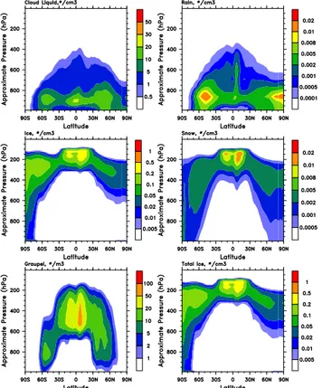
Figures 1 and 2 show annual average zonal mean latitude-pressure cross sections for grid-averaged hydrometeor mass and number concentrations, respectively. Simulated cloud liquid water mass concentrations peak over the tropics and mid-latitude storm tracks at 800–900 hPa, which is similar to the distribution of liquid droplet number concentrations, though the latter demonstrates the stronger influence of an-thropogenic aerosols as cloud droplet number concentrations are higher in the Northern Hemisphere (NH) than in the Southern Hemisphere (SH). Rain water is more concentrated over the tropics, though rain droplet number concentrations
Figure 01
Fig. 1. Annual-averaged zonal-mean grid-mean mass
concentra-tions (mg m−3)of cloud liquid water, rain water, ice water, snow water, graupel water, and total ice water (ice+snow+graupel) in PD in the MMF. The host GCM model (CAM5) uses a hybrid verti-cal coordinate and the pressure at the kth model level is given by
p(k) = A(k)p0+B(k)ps, where ps is surface pressure, p0 is a
specified constant pressure (1000 hPa), and A and B are coeffi-cients. Data are plotted as a function of this hybrid vertical coor-dinate times 1000, and labelled “Approximate Pressure”.
peak over the SH mid-latitudes and over the NH high lati-tudes, which indicates that rain droplet size is larger over the tropics than over the middle and high latitudes. As cloud for-mation over the high latitudes is mainly through large-scale cooling or moistening, but not strong convective motions, rain formation over the high latitudes is likely dominated by warm collision-coalescence processes and drizzle from low clouds rather than melting from graupel and snow, which ex-plains why rain mass mixing ratios are low but rain droplet number concentrations are high over the high latitudes.
Simulated cloud ice mass concentrations peak in the up-per troposphere over the tropics, while ice crystal number concentrations peak over both the tropics and high latitudes because of colder temperatures over these regions. Snow wa-ter mass dominates the total ice wawa-ter in the MMF model, as we discussed in Sect. 3.1, and graupel has a small con-tribution to the total ice water. The total ice water distri-bution shows a peak at 400–500 hPa over the tropics, and two other peaks over the mid-latitude storm track regions,
Figure 02
Fig. 2. The same as Fig. 1, but for hydrometeor number
concentra-tions (units: m−3for grauple, and cm−3for other hydrometeors).
which are in reasonable agreement with the total ice water distribution from CloudSat (Waliser et al., 2009; Gettelman et al., 2010). The spatial distributions of the different ice hy-drometeors are qualitatively similar to those from the NASA fvMMF (Fig. 12 in Waliser et al., 2009), except that the NASA fvMMF simulates a large contribution from graupel.
Figure 3 compares simulated annual-mean total cloud cover with the ISCCP observations. The total cloud cover in the MMF is diagnosed based on column-integrated to-tal cloud water path (liquid + ice) at each CRM column. Columns are considered cloudy if the total cloud water path is larger than 1 g m−2 and clear otherwise. The instan-taneous total cloud cover is defined as a ratio of cloudy columns to the total number of columns in the CRM (32 in the current setup). The simulated spatial pattern of to-tal cloud cover is in reasonable agreement with observa-tions, but in general, the model underestimates cloud frac-tion. The underestimation is especially pronounced over regions where low clouds dominate, such as over the sub-tropical regions in which trade cumulus and stratocumulus are observed. This underestimation, also evident in several previous MMF studies (Khairoutdinov et al., 2005, 2008), is caused in part by the coarse CRM horizontal resolution (4 km), which makes it difficult to simulate boundary layer clouds in the MMF model. We note that the threshold LWP of 1 g m−2roughly corresponds to a cloud optical depth (τ )
Figure 03
Fig. 3. PD annual average cloud fraction from the MMF model
(upper panel) and from the ISCCP observations (lower panel).
of 0.03–0.1 with droplet effective radius (Reff)varying from
15 to 5 µm, based on the following cloud optical depth for-mula: τ = 3LWP/(2Reff×ρw), where ρw denotes the liquid
water density. This threshold cloud optical depth is smaller than the detection threshold of the ISCCP, which is about 0.3. In future studies, we will apply instrumental simulators to provide a fairer comparison between models and satellite observations (e.g., Marchand and Ackerman, 2010).
Figure 4 compares simulated annual-mean shortwave and longwave cloud forcings with those from the CERES ob-servations. Shortwave (longwave) cloud forcing is defined as the difference between the shortwave (longwave) clear-sky and all-clear-sky radiative fluxes at the top of the atmo-sphere. Annual global mean shortwave cloud forcing in the MMF model is larger than the CERES observation (−50.5 vs. −47.1 W m−2). The MMF model underestimates short-wave cloud forcing over regions with a large amount of low clouds, such as over the subtropical regions, consistent with the underestimation of cloud cover (Fig. 3), while it overes-timates shortwave cloud forcing over the tropics. The long-wave cloud forcing in the MMF model is smaller than the CERES observation (26.0 vs. 29.9 W m−2). The radiative ef-fect of snow particles is accounted for in this study, following the same treatment as in CAM5 (Gettelman et al., 2010), and is included in the cloud forcing. The particle shape recipe was based on observations reported in Larson et al. (2006) at −45◦C: 7 % hexagonal columns, 50 % bullet rosettes and 43 % irregular ice particles. A sensitivity test with the MMF model at a coarse GCM resolution (4◦×5◦) shows that in-cluding the radiative effect of snow increases the shortwave cloud forcing by about 8 W m−2(in the absolute amount) and the longwave cloud forcing by 5 W m−2in January.
Figure 04
Fig. 4. PD annual average shortwave (left panels) and longwave (right panels) cloud forcing from the MMF model (upper panels) and from
the CERES observations (lower panels).
Precipitable water Precipitation rate
Precipitation rate
Figure 05
Precipitable water
Fig. 5. PD annual average precipitation rate (left panels) and precipitable water (right panels) from the MMF model (upper panels) and from
the observations (lower panels: precipitation rate from the GPCP observations and precipitable water from the NVAP observations).
Figure 5 compares simulated annual-mean precipitation rate and precipitable water with observations. The model re-produces the overall features of the observation. However, the model simulates excessive precipitation over the west Indian Ocean, the Maritime continent, Australia, West Pa-cific, East Pacific in the tropics, and west China. The model underestimates precipitation rates over ocean and over land in the subtropics and mid-latitudes. Simulated global pre-cipitation rate is 2.85 mm day−1, higher than observations (2.61 mm day−1). The simulated precipitable water distribu-tion has patterns similar to those in the observadistribu-tions. How-ever, the model overestimates precipitable water over most of
the oceans and the Maritime Continent, and underestimates precipitable water over land in the subtropics. The simula-tion of precipitasimula-tion and precipitable water by this version of the MMF model is quantitatively similar to the previous ver-sion of MMF (Khairoutdinov et al., 2008). The two-moment cloud microphysics coupled with a modal aerosol treatment in this version of the model does little to improve the simu-lations of precipitation and precipitable water.
Figure 6 compares simulated annual-mean cloud-top droplet number concentration with that from the MODIS satellite retrievals. The satellite data is derived from ver-sion 4 of the MODIS by Quaas et al. (2006), assuming
0 60E 120E 180 120W 60W 0 0 60N 90N 90S 60S 30S 30N Latitude MMF 0 60E 120E 180 120W 60W 0 0 60N 90N 90S 60S 30S 30N Latitude CAM5 MODIS 0 60E 120E 180 120W 60W 0 0 60N 90N 90S 60S 30S 30N Latitude Longitude
Figure 06Fig. 6. PD annual-averaged cloud-top droplet number
concentra-tions (cm−3)derived from the MMF (upper panel), CAM5 (middle panel) and MODIS (lower panel).
adiabatic clouds. For both the satellite and model data, only warm (temperature > 273 K) and low level clouds (pres-sure > 640 hPa) are sampled. For consistency, the model output is only sampled at the satellite overpass time (13:30 LST). The MMF model reproduces the spatial patterns of the observed cloud-top droplet number concentrations, with larger droplet number concentrations over land than over ocean and over the NH than over the SH, which clearly demonstrates the influence of anthropogenic aerosols. The patterns in gradients are replicated by both the MMF model as well as observations from the anthropogenic sources over land to its downwind sides over marine environments, e.g., Pacific, Atlantic, and Indian Ocean. The MMF model also simulates enhanced droplet number concentrations over the Southern Ocean (around 50◦S), consistent with MODIS ob-servations. However, the MMF model overestimates droplet number concentrations over many oceanic regions, such as the Indian Ocean, the tropical Atlantic Ocean and the tropical Pacific Ocean. In contrast, over the oceanic regions, CAM5 simulates fewer cloud droplets than the MMF, and agrees better with the MODIS observations. On the other hand, over the continental regions, CAM5 simulates more cloud droplets than the MMF and overestimates cloud droplet num-ber concentrations compared with the MODIS observations. The differences in simulated cloud-top droplet number con-centrations between CAM5 and the MMF are consistent with the differences in simulated CCN concentrations discussed in Sect. 3.2.
3.2 Aerosol fields
Simulated aerosol fields in the PD simulation were doc-umented and evaluated against observations in Wang et al. (2011) and here we briefly compare the MMF results with CAM5.
The annual, global mean aerosol sources, burdens, and lifetimes are summarized in Table 2. It is not surprising that sea salt and dust burdens are similar in the MMF and CAM5 since dust and sea salt emissions in the MMF are tuned so their burdens match the CAM5 burdens. Simulated BC, POM and SOA burden in the MMF (CAM5) are 0.14 (0.11) Tg, 1.04 (0.77) Tg, and 1.83 (1.40) Tg, respectively. The lower BC, POM and SOA burdens in CAM5 are due to their larger wet removal rates (not shown).
The simulated sulfate burden in the MMF is 1.05 Tg S, which is about twice that in CAM5 (0.53 Tg S). The lower sulfate burden in CAM5 is partly from a larger wet re-moval rate, as evident from its shorter lifetime, and partly from smaller sulfate production (42.5 Tg S yr−1 in CAM5 vs. 59.8 Tg S yr−1in the MMF). The latter is caused in part by differences in SO2wet removal. In the MMF, SO2 wet
removal occurs only by rain (which results in little removal below freezing), and the SO2 solubility is based its
effec-tive Henry’s law equilibrium at pH=5. In CAM5, SO2 wet
removal occurs by all precipitation, and the SO2uptake
fol-lows that of H2O2. Both differences produce stronger SO2
wet removal in CAM5. In a sensitivity test (reduced-SO2
-wet-removal), the same wet scavenging treatment of SO2as
that in the MMF is applied to CAM5. This increases the PD sulfate burden in CAM5 by 28 %.
Simulated SO2 and sulfate concentrations in the MMF
model have been evaluated against observations from the IM-PROVE sites in the United States, the EMEP sites in Europe, and the remote ocean network sites operated by the Univer-sity of Miami in Wang et al. (2011). Table 3 summarizes the model performance in these comparisons, along with the results from CAM5. The MMF model simulates SO2
con-centrations in better agreement with observations at the IM-PROVE and EMEP sites than CAM5, though the MMF still overestimates SO2concentrations by a factor of 1–2.
Sim-ulated sulfate concentrations are overestimated over the IM-PROVE and EMEP sites, and are underestimated over the re-mote ocean network sites. The MMF model simulates high sulfate concentrations over remote ocean areas and agrees slightly better with observations than CAM5.
Table 4 compares simulated AOD in both the MMF and CAM5 with observational data from the AERONET at sites in East and South Asia, Europe, Northern and Southern Africa, North and South America (See Fig. 22 in Wang et al. (2011) for the scatter plots between the MMF and obser-vations for each region). Both the MMF and CAM5 under-estimate AOD over most regions. The MMF model agrees slightly better with observations than CAM5, in terms of both
Table 2. Global annual budgets of sulfate, BC, POM, SOA, dust and sea salt in the PD and PI simulations of the MMF and CAM5. CAM5
results are in parenthesis. Dust and sea salt budgets are separated into fine mode (Aitken + accumulation) and coarse mode components. Units are days for lifetime, Tg for burdens and Tg yr−1for sources, except for sulfate where units are Tg S and Tg S yr−1for burdens and sources.
Sulfate BC POM SOA Fine Dust Coarse Dust Fine Sea Salt Coarse Sea Salt
PD 59.75 7.76 50.28 103.44 75.87 2295.20 122.82 3564.24 source (42.47) (7.76) (50.28) (103.44) (96.44) (2917.22) (157.17) (4627.10) PD 1.05 0.14 1.04 1.83 2.00 19.40 0.88 11.29 burden (0.53) (0.11) (0.77) (1.40) (2.00) (21.64) (0.95) (10.77) PD 6.41 6.59 7.55 6.46 9.62 3.09 2.62 1.17 lifetime (4.55) (5.14) (5.59) (4.94) (7.57) (2.71) (2.21) (0.85) PI 25.82 3.08 31.64 92.68 83.84 2536.11 124.73 3590.88 source (15.24) (3.08) (31.64) (92.68) (101.07) (3057.35) (156.49) (4605.44) PI 0.45 0.06 0.67 1.57 2.16 21.13 0.86 11.11 burden (0.17) (0.04) (0.46) (1.21) (2.07) (22.63) (0.92) (10.63) PI 6.36 7.11 7.73 6.18 9.40 3.04 2.52 1.13 lifetime (4.07) (4.74) (5.31) (4.77) (7.48) (2.70) (2.15) (0.84) PD/PI 1.01 0.93 0.98 1.04 1.02 1.01 1.04 1.02 lifetime (1.12) (1.09) (1.05) (1.04) (1.01) (1.00) (1.03) (1.01)
Table 3. Observed means, normalized mean biases (b) and correlation coefficients (R) between models and observations for SO2, and SO4. Annual average data is used. Observations are from the United States Interagency Monitoring of Protected Visual Environment (IMPROVE) sites (http://vista.cira.colostate.edu/improve/), the European Monitoring and Evaluation Programme (EMEP) sites (http://www.emep.int), and the ocean network sites operated by the Rosenstiel School of Marine and Atmospheric Science (RSMAS) at the University of Miami (Prospero et al., 1989; Savoie et al., 1989, 1993; Arimoto et al., 1996). See Figs. 9–10 in Wang et al. (2011) for the scatter plots of MMF results versus observations.
SO2from IMPROVE SO2from EMEP SO4from IMPROVE SO4from EMEP SO4from RSMAS
Obs (mean) 0.30 0.77 1.59 2.37 0.94
MMF b 1.7 0.45 0.33 0.07 −0.10
CAM5 b 2.7 1.06 0.38 0.01 −0.33
MMF R 0.59 0.72 0.95 0.79 0.95
CAM5 R 0.56 0.68 0.96 0.74 0.97
normalized mean bias and correlation coefficients with ob-servations.
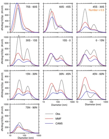
Figure 7 shows aerosol size distributions in the marine boundary layer. The observational data are from Heintzen-berg et al. (2000) and were compiled and aggregated onto a 15◦×15◦grid. The model output is sampled over the same regions as observations. Aerosol size distributions simulated by both the MMF and CAM5 are in reasonable agreement with observations, and show bimodal distributions in most regions. Simulated aerosol number concentrations in the MMF are higher than that in CAM5 and agree better with observations. Higher aerosol number concentrations in the MMF are consistent with its higher global aerosol burdens (Table 2). We note that cloud-top droplet number concentra-tions over the oceanic regions in CAM5 are lower than those in the MMF and agree better with the MODIS observation
(Fig. 6 in Sect. 3.1), which seems not consistent with the comparison shown in Fig. 7. However, the spatial and tem-porary coverage between satellite and field observations is different (e.g., field observations only cover a particular pe-riod, while MODIS has multi-year continuous observations). Moreover, the aerosol size distribution observations in Fig. 7 were made near the surface, while cloud droplet number con-centration from MODIS is at cloud top. These differences make it challenging to establish consistent pictures among different comparisons.
Figure 8 shows monthly BC concentrations at four sites in the polar regions. BC concentrations in the MMF are in rea-sonable agreement with observations, in terms of both mag-nitudes and seasonal cycles. In contrast, CAM5 underesti-mates BC concentrations by 1–2 orders of magnitude in the polar regions. What is more, CAM5 does not capture the
Table 4. Observed means, normalized mean biases (b) and correlation coefficients (R) between the model and observations for AOD over
seven different regions (North America, Europe, East Asia, North Africa, and South Africa, South Asia) and the global. Monthly mean data is used. Observations are from the AERONET sites (http://aeronet.gsfc.nasa.gov/). See Fig. 22 in Wang et al. (2011) for the scatter plots of MMF results versus observations.
North Europe East North South South South Global
America Asia Africa Africa America Asia
Obs (mean) 0.13 0.18 0.34 0.51 0.18 0.21 0.39 0.21 MMF b 0.10 −0.24 −0.35 −0.20 −0.30 0.03 −0.47 −0.13 CAM5 b −0.14 −0.37 −0.46 −0.27 −0.25 0.03 −0.62 −0.24 MMF R 0.91 0.37 0.37 0.37 0.67 0.51 0.56 0.74 CAM5 R 0.88 0.22 0.32 0.38 0.58 0.51 0.77 0.69 Diameter (nm) Diameter (nm) Diameter (nm) Figure 07
Fig. 7. PD aerosol size distributions in the marine boundary layer
from the MMF, CAM5, and observations. Observations (Obs) are from Heintzenberg et al. (2000). For the 45◦S–30◦S latitude band, aerosol number density is scaled by 0.5 so the same y axis can be used for all latitude bands.
observed seasonal cycle. Simulated sulfate aerosols over the Arctic in the MMF demonstrate a similar improvement over CAM5 (not shown).
Figure 9 shows the annual mean global distribution of CCN concentrations (at 0.1 % supersaturation) averaged over the lowest 8 model levels (surface to about 800 hPa) in both
2 4 6 8 10 12 10−2 10−1 100 101 South Pole BC(ng/m3) Month 89.0S 102.0W 2 4 6 8 10 12 10−2 10−1 100 101 Halley, Antarctica Month 75.6S 26.2W 2 4 6 8 10 12 10−2 100 102 104 Barrow, Alaska BC(ng/m3) Month 71.2N 156.3W MMF CAM5 2 4 6 8 10 12 10−2 100 102 104 Alert, Canada Month 82.5N 62.3W
Figure 08Fig. 8. Monthly-average BC concentrations at four polar sites: (a) Amundsen-Scott, South Pole (Bodhairne, 1995); (b) Halley,
Antarctica (Wolff and Cachier, 1998); (c) Barrow, Alaska (Bod-haine, 1995); and (d) Alert, Canada (Hopper et al., 1994). PD model results are in solid lines (red: MMF; blue: CAM5), and ob-served data are in dots.
the MMF and CAM5. The spatial patterns of CCN concen-trations are similar in the MMF and CAM5, with high con-centrations over strongly polluted regions, and low concen-trations over remote regions. However, the MMF produces lower CCN concentrations in the strongly polluted regions and higher CCN concentrations in the remote regions, such as remote oceanic regions and polar latitudes, than CAM5. The higher CCN concentrations in the polar latitudes in the MMF can also be seen in the annual zonal distribution shown in Fig. 10, which is consistent with higher aerosol concen-trations in the polar latitudes discussed above (Fig. 8). It is also evident in Fig. 10 that the MMF produces higher CCN concentrations at high altitudes than CAM5. Differ-ences in convective transport, wet scavenging in stratiform
∆CCN/CCNPI, MMF ∆CCN/CCNPI, CAM5
∆CCN, MMF Mean: 30.84 cm-3 ∆CCN, CAM5 Mean: 32.90 cm-3
Figure 09
CCN, PD, MMF Mean: 95.25 cm-3 CCN, PD, CAM5 Mean: 90.48 cm-3
Fig. 9. Annual-averaged global distribution of CCN concentrations at 0.1 % supersaturation averaged over the lowest 8 model levels (surface
to about 800 hPa) in the PD simulations (top panels), the difference between PD and PI (PD-PI) (middle panels), and the relative differences between PD and PI [(PD-PI)/PI] (bottom panels) in both the MMF (left panels) and CAM5 (right panels).
MMF CAM5
Figure 10
Fig. 10. Annual-averaged zonal-mean CCN concentrations at 0.1 %
supersaturation in the PD simulations in the MMF (left panel) and CAM5 (right panel).
and convective clouds, and long range transport between the MMF model and CAM5 may lead to these differences. Fur-ther studies are needed to identify the causes for the differ-ences between the MMF and CAM5.
4 Aerosol indirect effects
4.1 Aerosol-cloud relationships in the PD
Following Quaas et al. (2009), the strength of aerosol-cloud interactions (ACI) is defined as the relative change in cloud properties with respect to the relative change in aerosol opti-cal properties, and is opti-calculated as:
ACI =dlnC dlnA,
where C is a cloud parameter (e.g., cloud droplet number concentration, cloud LWP, or cloud fraction), and A is a proxy for column-integrated CCN concentrations. Quaas et al. (2009) used AOD as the proxy for column-integrated CCN concentrations. Aerosol Index (AI), which is the prod-uct of AOD and ˚Angstr¨om coefficient, has also been used in some previous studies as a surrogate for the column-integrated CCN concentrations. Compared to AOD, AI is more representative of the column-integrated CCN concen-trations since the ˚Angstr¨om coefficient accounts for the par-ticle size with smaller ˚Angstr¨om coefficients for larger size
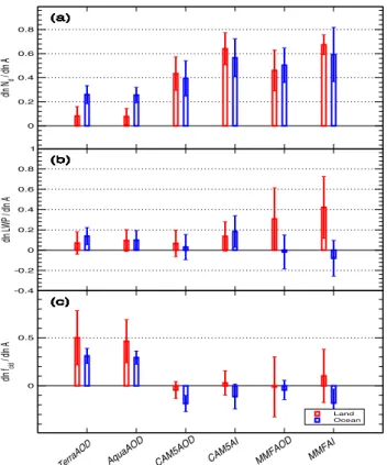
TerraAOD AquaAOD CAM5AOD CAM5AI MMFAOD MMFAI 0 0.5 dln fcld / dln A Land Ocean -0.4 -0.2 0 0.2 0.4 0.6 0.8 1 dln LWP / dln A 0 0.2 0.4 0.6 0.8 dln Nd / dln A (c) (c) (c) (c) (c) (c) (c) (c) (c) (c) (c) (c) (c) (c) (c) (c) (c) (c) (b) (c) (b) (c) (b) (c) (b) (c) (b) (c) (b) (c) (b) (c) (b) (c) (b) (c) (b) (c) (b) (c) (b) (c) (b) (c) (b) (c) (b) (c) (b) (c) (b) (c) (b) (a) (c) (b) (a) (c) (b) (a) (c) (b) (a) (c) (b) (a) (c) (b) (a) (c) (b) (a) (c) (b) (a) (c) (b) (a) (c) (b) (a) (c) (b) (a) (c) (b) (a) (c) (b) (a) (c) (b) (a) (c) (b) (a) (c) (b) (a) (c) (b) (a) Figure 11
Fig. 11. Sensitivities of (a) cloud-top droplet number
concentra-tion, (b) cloud liquid water path, (c) cloud fraction to perturbations in column-integrated aerosol number concentration proxies repre-sented by either AOD or AI as obtained from the linear regres-sions in PD. The weighted averages for four seasons and all six land regions (red) and eight ocean regions (blue) are show, with the variability as error bar. Results are shown for MODIS Terra (Ter-raAOD: cloud parameters vs. AOD); MODIS Aqua (AquaAOD: cloud parameters vs. AOD); CAM5 (CAM5AOD: cloud parameters vs. AOD, CAM5AI: cloud parameters vs. AI); MMF (MMFAOD: cloud parameters vs. AOD, MMFAI: cloud parameters vs. AI).
particles (Nakajima et al., 2001). Here both AOD and AI are used as proxies for the column-integrated CCN concentra-tions to calculate ACI in the MMF model for cloud droplet number concentrations, LWP, and cloud fraction, following the same approach as that in Quaas et al. (2009). ACI is ob-tained by a linear regression between lnC and lnA. Model output is sampled daily at 01:30 p.m. local time to match the MODIS Aqua equatorial crossing time. The model out-put is interpolated to a 2.5◦×2.5◦regular longitude-latitude
grid as in Quaas et al. (2009), to facilitate the direct com-parison between the current study and Quaas et al. (2009). The regressions for the MMF and CAM5 simulations are performed separately for fourteen different ocean and land regions and four seasons as in Quaas et al. (2009). We com-pare the MMF results with those from the standard CAM5, and those from the observations and other model results in Quaas et al. (2009).
Figure 11 shows the mean sensitivities of cloud param-eters to column aerosol properties for all seasons in both the land and ocean areas from the satellite data, and from the MMF and CAM5 simulations, with the error bars show-ing the variability among 6 land or 8 ocean regions and 4 seasons. Cloud-top droplet number concentration increases with increasing AOD in both models and satellite observa-tions (Fig. 11a). Simulated slopes between cloud-top droplet number concentration and AOD in the MMF and CAM5 are similar, with a slightly larger slope in the MMF, and are sig-nificantly larger than that in satellite observations. We note that half of the global climate models included in Quaas et al. (2009) overestimated the slope. Replacing AOD with AI in the MMF and CAM5 further increases the slope, which is consistent with McComiskey et al. (2009).
The slope between LWP and AOD is positive over land in the MMF model, consistent with those in satellite ob-servations and CAM5, but the magnitude is larger in the MMF than in the satellite observations and in CAM5. In contrast, LWP and AOD over ocean are negatively corre-lated in the MMF, which is opposite to those in CAM5 and the MODIS retrievals. Replacing AOD with AI leads to larger negative/positive slope over ocean/land for the MMF. Both positive and negative correlations between LWP and AOD/AI have been observed (Platnick et al., 2000; Coak-ley and Walsh, 2002; Kaufman et al., 2005; Matsui et al., 2006). Using a global CRM with on-line aerosols, Suzuki et al. (2008) also obtained a negative correlation between LWP and AI from an 8-day integration in July. The positive corre-lation between LWP and AOD/AI is attributed to cloud life-time effects from aerosols or/and aerosol swelling effects in the high relative humidity regions surrounding clouds. The negative correlation between LWP and AOD/AI can be at-tributed to rain wash-out effects (Suzuki et al., 2004), semi-direct effects (Hansen et al., 1997), or dynamical feedbacks such as enhanced entrainment of drier air or enhanced evap-oration of the more numerous smaller cloud droplets in pol-luted clouds (Ackerman et al., 2004; Jiang et al., 2006). Our results suggest that the negative effect dominates over ocean while the positive effect dominates over land in the MMF model.
Simulated cloud fraction and AOD are negatively corre-lated in the MMF and CAM5, opposite to the correlation found in the satellite retrievals, though using AI instead of AOD leads to a slightly positive correlation over land in both models. The positive correlation in satellite data can be attributed to the swelling of aerosol particles near clouds, cloud lifetime effects from aerosols, or the contamination in AOD retrievals by clouds. Quaas et al. (2010) showed that the positive correlation between cloud fraction and AOD in their model can largely be attributed to the aerosol swelling effects, and a negative correlation is found when dry AOD is used. The negative correlation between cloud fraction and AOD in CAM5 and the MMF may indicate the stronger scavenging effects of clouds on aerosols and/or less swelling
ΔCDR, MMF Mean: -0.53 μm ΔCDNC, MMF Mean: 24.4 cm-3 ΔCDR, CAM5 Mean: -0.44 μm ΔCDNC, CAM5 Mean: 29.7 cm-3 La titude La titude Longitude Longitude Figure 12
Fig. 12. Annual-average changes (PD–PI) in cloud-top droplet number concentrations (upper panels) and cloud-top droplet effective radius
(lower panels) between the PD and PI simulations for low level (pressure >640 hPa), warm clouds (cloud top temperature warmer than 273.16 K) in the MMF (upper panel) and CAM5 (lower panel).
effects of clouds on aerosols in both models. We note that the MMF AOD is from the clear-sky CRM columns and therefore may be less susceptible to the swelling effects than CAM5 AOD.
4.2 Anthropogenic aerosol effects
4.2.1 Anthropogenic aerosol effects in the MMF
As summarized in Table 2, simulated aerosol loadings have increased significantly since preindustrial time. Globally, sulfate, BC, POM, and SOA burdens increase by 133 %, 133 %, 55 %, and 17 %, respectively from the PI to PD. Dust and sea salt burden are similar in both PI and PD simula-tions. The lifetimes of sulfate, SOA, dust and sea salt in-crease slightly from PI to PD, which may be caused in part by cloud lifetime effects from aerosols (more aerosols lead to longer cloud lifetime, and therefore less efficient wet re-moval in PD than in PI), a positive feedback in aerosol in-direct effects. On the other hand, the lifetimes of BC and POM decrease from PI to PD, which may be caused in part by enhanced sulfate coating on BC and POM and therefore enhanced wet removal of BC and POM in the PD.
Figure 12 shows the global distribution of changes in annual-mean cloud-top droplet number concentrations (CDNC) and cloud-top droplet effective radius (CDR) be-tween the PD and the PI simulations (PD-PI). Cloud-top droplet number concentrations increase from the PI to PD simulations over most regions, and increases in cloud-top droplet number concentrations are mainly located in the
source regions of fossil fuel burning (e.g., more than 50 cm−3 in Europe, East and South Asia) and biomass burning (e.g., more than 30 cm−3in Africa and South America), and down-wind of the source regions (e.g., between 10–30 cm−3 in the mid-latitude Pacific and the tropical Atlantic). De-creases in droplet number concentrations are simulated in some regions, such as Southeast United States, central South America, and North Australia, which are caused by re-duced biomass burning emissions from PI to PD (not shown). Cloud-top droplet effective radius decreases from the PI to PD simulations over most regions, by more than 1 µm over strongly polluted regions (e.g., East and South Asia) and more than 0.5 µm over many oceanic regions (e.g., the North Pacific). The spatial pattern of changes in droplet effective radius is consistent with the spatial pattern of changes in cloud-top droplet number concentrations (i.e., large increases in droplet number concentrations lead to large decreases in droplet effective radius).
Figure 13 shows the zonal distribution of changes in AOD, cloud liquid water path (LWP), CDR, CDNC, shortwave cloud forcing (SWCF), and net total fluxes (shortwave + longwave) at the top of the atmosphere (FSNT+FLNT) between the PD and PI simulations. In-creases in AOD from the anthropogenic aerosols are mainly located north of 30◦S, and peak in the NH mid-latitudes with a value of about 0.04. Increases in cloud-top droplet number concentrations closely follow the changes in AOD, with a peak of about 40 cm−3in the NH mid-latitudes. De-creases in cloud-top droplet effective radius are larger over the NH mid-latitudes, consistent with the large increases
Latitude Latitude e) ΔSWCF (W/m2) b) ΔLWP (g/m2) a) ΔAOD c) ΔCDR (micrometer) d) ΔCDNC (#/cm3) Figure 13 f) Δ(FSNT+FLNT) (W/m2)
Fig. 13. Change in the zonal-mean annual-average (a) AOD, (b)
liq-uid water path (LWP), (c) cloud top droplet effective radius (CDR),
(d) cloud top droplet number concentrations (CDNC); (e) shortwave
cloud forcing (SWCF); and (f) net total flux at the top of the at-mosphere (FSNT+FLNT) from anthropogenic aerosols in both the MMF (red lines) and CAM5 (blue lines) simulations.
in cloud-top droplet number concentration, and also larger over the NH high latitudes, which can be explained by the large relative changes in cloud-top droplet number concen-trations. Increases in LWP are large over the tropics and the NH mid-latitudes, which is consistent with the increases in cloud droplet number concentrations over these regions. On the other hand, changes in LWP in the NH subtropics and the latitude bands around 60◦N are small though changes in cloud-top droplet number concentrations are large over these regions. Increases in the shortwave cloud forcing (in the ab-solute amount) are caused by both decreases in droplet ef-fective radius and increases in LWP, while its changes fol-low more closely with changes in LWP than with changes in droplet effective radius (e.g., smaller changes in the NH subtropics and around 60◦N). The positive change in short-wave cloud forcing at around 20◦N is caused by a decrease in cloud fraction (not shown). Changes in net total fluxes at the top of the atmosphere are larger in the NH than in the SH. The global mean changes from the PI to PD simula-tions are summarized in Table 5. Globally, anthropogenic aerosols lead to a 0.024 increase in clear-sky AOD, a 24 cm−3 increase in cloud-top droplet number concenttions, a 0.52 µm decrease in cloud-top droplet effective ra-dius, and a 2.11 g m−2 increase in LWP. A cooling of 0.77 W m−2in shortwave cloud forcing is simulated, which results from the decreases in cloud droplet effective radius and increases in liquid water path. As expected, simulated longwave cloud forcing has little change between the PD
and PI simulations since aerosol effects on ice clouds are not accounted for in this version of the MMF model. Sim-ulated total aerosol effect on the shortwave fluxes at the top of the atmosphere is −1.31 W m−2. The aerosol ef-fect in the clear-sky (assuming entirely clear grid boxes) is −0.54 W m−2. The simulated aerosol effect on the net total fluxes (shortwave + longwave) is −1.05 W m−2, with a long-wave contribution of 0.26 W m−2. The longwave warming of 0.26 W m−2is mainly from the contribution in the clear sky, which is caused in part by cooling over land surface (surface temperature over land decreases by 0.34 K) and therefore less thermal emission from land.
4.2.2 Comparison with CAM5
In the standard version of CAM5, the simulated PI to PD change in shortwave cloud forcing is −1.79 W m−2, the
change in longwave cloud forcing is 0.37 W m−2, the aerosol
direct effect in shortwave fluxes in the clear sky (taking into account entirely clear grid boxes) is −0.45 W−2, and the aerosol effect on the net total fluxes (FSNT + FLNT) is −1.66 W m−2. The larger clear-sky direct effect in the MMF than in CAM5 (−0.54 W m−2in the MMF vs. −0.45 W m−2 in CAM5) can be explained in part by the larger increase in sulfate burden from PI to PD in the MMF (0.60 Tg S) than in CAM5 (0.36 Tg S). We also noted that aerosol water uptake in the MMF is calculated at each CRM grid cell with a CRM-scale relative humidity, while aerosol water uptake in CAM5 is calculated at each GCM grid cell with a GCM-scale clear-sky relative humidity. This may be another reason why the MMF simulates the larger clear-sky direct effects, since in-cluding subgrid variations in the relative humidity can lead to larger aerosol direct effects because of the nonlinear de-pendence of aerosol water uptake on relative humidity (Hay-wood et al., 1997).
The simulated change in shortwave cloud forcing in the MMF (−0.77 W m−2) is much smaller than that in CAM5 (−1.79 W m−2), despite the fact that changes in AOD and cloud-top droplet effective radius from anthro-pogenic aerosols in the MMF are slightly larger than those in CAM5 (Table 3 and Figs. 12–13). For example, the global, annual mean change in cloud-top droplet effective ra-dius is −0.53 µm in the MMF simulations, compared with −0.45 µm in the CAM5 simulations (Table 3 and Fig. 12).
The smaller change in shortwave cloud forcing in the MMF is consistent with its smaller change in liquid water path (LWP) between the PI and PD simulations (Fig 13b). Globally, an increase of 3.9 % in LWP from PI to PD is sim-ulated in the MMF, which is about one-fourth of the change of 15.6 % in LWP in stratiform clouds (and about half of the change of 8.8 % in total LWP) in CAM5. Regionally, the LWP in stratiform clouds in CAM5 increases by more than 50 % over many continental regions with strong anthro-pogenic emissions (e.g., East Asia, South Asia, the Maritime Continent, and Europe) and increases by more than 20 %
Figure 14.
∆LWP/LWPPI, MMF ∆LWP/LWPPI, CAM5
∆LWP, MMF Mean: 2.11 g m-2 ∆LWP, CAM5 Mean: 4.04 g m-2 LWP, PD, MMF Mean: 55.99 g m-2 LWP, PD, CAM5 Mean: 29.95 g m-2
Fig. 14. Annual-averaged global distribution of liquid water path (LWP) in the PD simulations (top panels), the difference between PD and
PI (PD–PI) (middle panels), and the relative differences between PD and PI [(PD–PI)/PI] (bottom panels) in both the MMF (left panels) and CAM5 (right panels). Liquid water path in CAM5 is from large-scale clouds only and does not include contributions from convective clouds.
over some oceanic regions such as the North Pacific Ocean (Fig. 14). In contrast, the increase in LWP in the MMF is much weaker, less than 30 % over most continental regions, and less than 10 % over most oceanic regions. It is evident in Fig. 13 that the large differences in simulated aerosol in-direct effects between the MMF and CAM5 occur over the regions where the differences in changes of LWP are larger such as over the NH subtropics (compare Fig. 13e to b). The scatter plots of the relative change in LWP and in shortwave cloud forcing shown in Fig. 15 further demonstrate that the larger change in LWP in CAM5 leads to the larger change in shortwave clouds forcing.
The much smaller increase in LWP in the MMF is caused primarily by a much smaller response in LWP to a given CCN perturbation from PI to PD as shown in Fig. 16a–b. The slope between the relative change in LWP and the rel-ative change in CCN from the linear regression is 0.11 in the MMF and is 0.30 in CAM5, which indicates that the re-sponse in LWP to a given CCN perturbation in the MMF is about one-third of that in CAM5.
The smaller increase in LWP in the MMF is also caused, to a lesser extent, by a smaller relative increase in CCN con-centrations in the MMF from PI to PD, as shown in Fig. 16c. The relative changes in CCN concentrations from PI to PD in CAM5 are about 35 % larger than that in the MMF. This is consistent with Figs. 9 and 14, which show that changes in both CCN concentrations and LWP are weaker in the MMF. The smaller relative increases in CCN concentrations in the MMF can be partly explained by the changes in aerosol times between the PD and PI simulations (Table 2). The life-time of sulfate aerosol has little change from the PI to PD simulations in the MMF, but increases by 12 % in CAM5. The lifetime of BC decreases by 7 % from the PI to PD sim-ulations in the MMF, while it increases by 9 % in CAM5. The large increase in sulfate and BC lifetimes in CAM5 from the PI to PD simulations can be explained in part by the positive feedback in aerosol indirect effects due to cloud lifetime effects from aerosols (more aerosols lead to longer cloud lifetime and therefore less wet scavenging, which in turn increases CCN concentrations). This positive feedback
Figure 15
Y=0.50*X+0.0 Y=0.42*X+0.0
Fig. 15. Scatter plots and regressions of the relative changes
[(PD-PI)/PI] in annual-mean shortwave cloud forcing (SWCF) versus the relative changes in annual-mean liquid water path (LWP) in both the MMF (left panel) and CAM5 (right panel) from PI to PD. Annual mean model data are sampled on each GCM grid column from 60◦S to 60◦N. LWP in CAM5 includes contributions from both large-scale and convective clouds. Red lines and equations are from the linear regression.
induced by cloud lifetime effects from aerosols is stronger in CAM5 than in the MMF, partly due to the larger increase in LWP in CAM5. The smaller relative increase in CCN con-centrations in the MMF is also partly caused by the smaller relative increase in sulfate sources in the MMF (Table 2). The sulfate source increases by 130 % from PI to PD in the MMF, while it increases by 178 % in CAM5. This is partly caused by the changes in the lifetime of SO2, which
de-creases by 14 % from PI to PD in the MMF, while inde-creases by 20 % in CAM5. The differences in changes in sulfate source and SO2 lifetime from PI to PD result from
differ-ences in the treatment of wet removal of SO2(less efficient
wet removal of SO2 in the MMF), differences in the
mag-nitude of cloud lifetime effects from aerosols (weaker cloud lifetime effects in the MMF) and differences in the treatment of aqueous chemistry (a fixed pH value of 4.5 in the MMF versus a SO4-dependent pH value in CAM5) (Wang et al.,
2011; Liu et al., 2011).
The higher sulfate burdens in the MMF versus CAM5 do not appear to contribute significantly to different LWP re-sponse to a given CCN perturbation and the stronger indirect effect in CAM5. In the reduced-SO2-wet-removal
sensitiv-ity test (see the discussion in Sect. 3.2 about the sensitivsensitiv-ity test and the differences in the treatment of SO2wet removal
between the MMF and CAM5), reducing SO2wet removal
has little effect on simulated LWP response to a given CCN perturbation and slightly increases aerosol indirect forcing in CAM5, even though it increases the PD and PI sulfate bur-dens by 28 % and 40 %, respectively.
To further examine how clouds with different LWP re-spond differently to anthropogenic aerosols, Fig. 17 shows the probability density function (PDF) of in-cloud LWP over the globe in the PD simulations and the relative changes in this PDF from the PI to PD simulations in both the MMF
and CAM5. Model output (34 months data for the MMF and 4 yr data for CAM5) are sampled daily at 01:30 pm lo-cal time. The in-cloud LWP in CAM5 is derived from the grid-mean LWP and the liquid cloud cover calculated based on the same maximum/random cloud overlap assumption as used in the radiative transfer calculation in CAM5. The PDFs of LWP calculated from in-cloud LWP at each GCM column in both the MMF and CAM5 (Fig. 17c and d) are weighted by cloud cover. In-cloud LWP in CAM5 includes a contribution from stratiform clouds only, while in-cloud LWP in the MMF includes contributions from both stratiform and convective clouds. The PDFs of LWP in PD show that the frequency of occurrence of LWP decreases with increasing LWP and that clouds with LWP larger than 200 g m−2occur more often in the MMF than in CAM5 (Fig. 17a).
The relative changes in the PDF of LWP (green lines in Fig. 17b–d) show that cloud fraction of thin clouds decreases and that cloud fraction of thick clouds increases in both the MMF and CAM5 from the PI to PD simulations (relative changes in the frequency of occurrence at a given LWP bin is equivalent to relative changes in cloud fraction at that given LWP bin). It is also evident in Fig. 17b–d that increases in cloud fraction in thick clouds accelerate with increasing LWP bins. For example, the decreases in cloud fraction can reach as high as 2 % for the smallest LWP bins, while the increase in cloud fraction can be larger than 10 % for clouds with LWP larger than 1000 g m−2in the MMF. The differ-ent responses of thin and thick cloud LWP to anthropogenic aerosol perturbations can be explained in part by cloud life-time effects from aerosols. Thick clouds are more likely to precipitate and therefore their LWP are more suscepti-ble to anthropogenic aerosol perturbations. The accelerat-ing increase in cloud fraction for thick clouds with increas-ing LWP may partly result from the autoconversion scheme used in the models, which is based on Khairoutdinov and Kogan (2000). The autoconversion rate in the Khairoutdinov and Kogan scheme has a strong dependence on liquid water content (qc2.47), which leads to a strong dependence of the relative autoconversion rate (the autoconversion rate divided by liquid water content) on liquid water content (qc1.47)and therefore larger relative increases in cloud fraction for clouds with larger LWP. On the other hand, thin clouds are less likely precipitating and their LWPs are therefore less suscep-tible to anthropogenic aerosol perturbations. Other factors, such as semi-direct effects and dynamical feedbacks (e.g., entrainment drying, Ackerman et al., 2004) can even lead to a decrease in cloud fraction for these thin clouds.
Figure 17 also further demonstrated that the response in LWP to anthropogenic aerosol perturbation is much larger in CAM5 than in the MMF, consistent with Fig. 16. In CAM5, cloud fraction increases for clouds with in-cloud LWP larger than 50 g m−2and increases by more than 20 % for clouds with LWP larger than 200 g m−2, and more than 50 % for clouds with LWP larger than 400 g m−2, which are much larger than those in the MMF. The larger response in LWP