Polymer Aging Mechanics
An investigation on a Thermoset Polymer used in
the Exterior Structure of a Heavy-duty Vehicle
Master’s Thesis
Abstract
The use of plastic materials in the design of vehicle components is primarily driven by the need for vehicle weight and cost reduction. Additionally, these materials give design engineers freedom in creating appealing exterior designs. However, creating self-carrying exterior structures with polymers must fulfil long-term strength, creep and fatigue life requirements. Thus, the polymer polyDicyclopentadiene (pDCPD) has been chosen for this purpose. Its aging mechanics need to be understood by the design engineers to make the right decisions. This thesis has carried out mechanical tests such as uniaxial tensile testing, fatigue, and creep testing. Digital image correlation (DIC) system has been used to capture strain data from tensile tests. In the final analysis, DIC measurements proved more accurate than extensometer data retrieved from the testing machine. The rise in temperature has been captured using thermal imaging. Several degradation processes have been explored including physical aging, thermo-oxidation, photo-oxidation, chemical- and bio- degradations. Test results showed significant changes in mechanical properties after 17 years of aging. Additionally, severe thermal degradation has been observed in one of the tested panels of pDCPD. Temperature can rise to significant levels during cyclic loading at high stresses, which could have an impact on physical aging effects. Viscoelastic behavior has been explored and changes in dynamic and creep properties have been observed. The investigation also reviled that different defects caused by flawed manufacturing also can affect the material severely as one case has proved in this research.
Keywords: polyDicyclopentadiene; aging; thermosets; fatigue; mechanical
properties; thermal fatigue; digital image correlation; viscoelasticity; polymer degradation; thermo-oxidation; photo-oxidation.
Acknowledgments
First and foremost, I would like to thank my supervisor Professor Torbjörn Ekevid, for his help, knowledge, and support during this work. This thesis topic was proposed by him through his work at Volvo Construction Equipment in Braås, Sweden. Thank you for giving me the opportunity and trust to work under your supervision and for all the advice and support you provided throughout this research project.
Furthermore, I would like to thank Senior Lecturer Peter Lerman for providing equipment and for his guidance throughout this master program. A special thanks to Bertil Enquist and Jonas Klaeson for their mentorship, help, and support during laboratory work.
I offer my heartfelt gratitude to my family: My parents, and to Ali, Yussor & Alaa, for their perpetual and unconditional support, and of course, to my friends who’ve been there along the way.
Basil H. A. Abu-Ragheef 7th of June 2019
Table of contents
1 Introduction 1
1.1 Background 1
1.2 Problem Description 5
1.3 Purpose and Research Questions 5
1.4 Objectivity, Reliability, and Validity 6
2 Literature Review 7
2.1 An Overview of the Thermoset polyDicyclopentadiene (pDCPD) 7
2.2 Physical Aging in Polymers 9
2.3 Other Polymer Degradation and Aging Processes 12
2.3.1 Thermo-oxidation 12
2.3.2 Photo-oxidation and UV degradation 13
2.3.3 Biodegradation 14
2.3.4 Wet Environments and Water Absorption 14
2.4 Tensile and Plastic Behaviors in Polymers 15
2.5 Fatigue Behavior in Polymers 17
2.5.1 Thermal Fatigue 17
2.5.2 Mechanical Fatigue 19
3 Theory 21
3.1 Linear Elasticity and Stress-Strain Relations 21
3.2 Cyclic Stresses 25
3.3 Viscoelastic Behavior of Polymers 28
4 Methods 33
4.1 Determination of Tensile Properties 33
4.1.1 Uniaxial Tension Testing 33
4.1.2 Creep Testing 34
4.1.3 Digital Image Correlation (DIC) 34
4.2 Mechanical and Thermal Fatigue 35
4.2.1 Cyclic Tension Test 35
4.2.2 Thermography 35
4.3 Statistical Approaches 36
4.3.1 Regression Analysis 36
4.3.2 Bootstrap Confidence Intervals 37
4.4 Failure Analysis through Visual Examination 38
4.5 Experimental Implementation 39
4.5.1 Specimens Preparation 39
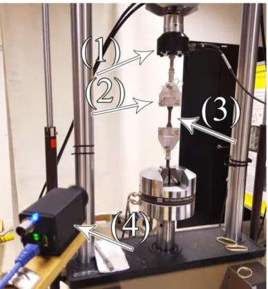
4.5.2 Testing Setup 40
4.5.3 Data Preparation and Analysis 43
5 Results and Analysis 44
5.1 Uniaxial Tensile Test Results 44
5.2 Analysis of Fatigue Test Results 49
5.4.2 Cyclic Stress and Strain Behavior 60
5.5 Thermal Behavior During Cyclic Stress Tests 64
6 Discussion 67
7 Conclusion 69
References 70
Appendix 1: Material Sheets 76
Appendix 2: Detailed Spreadsheet for each specimen ID 78
Appendix 3 Other test results 81
Appendix 4: DIC system results for strain analysis 89
1 Introduction
1.1 Background
Plastics have been frequently used materials by product designers and engineers for over a century due to its wide range of properties and its low-energy, fast production processes (Rosato, 2003). The automotive sector has used plastics since the early 1900s. The first notable use of plastics was during the second world war period when Henry Ford manufactured the “Soybean”, a plastic-bodied car made from agricultural plastic. (Ford et al., 1942; as cited in Pradeep et al., 2017.; The Henry Ford, 2019). Advancements in materials such as polymer composites have led to boosting fuel economy as it takes less energy to operate a lightweight vehicle than a heavy one (EERE, 2019). The automotive manufacturers have been pushing towards integrating plastics in the vehicle design to boost sustainability, improve manufacturing processes, reduce cost. Reducing weight, also increase performance and decrease harmful emissions (Erhard, 2006; Serrenho et al., 2017; Plastics Market Watch, 2016; Pervaiz et al., 2016). This has led the automotive industry to be accounted for 10% of plastic converters demand in Western Europe as of 2016 (PEMRG, 2017). These plastic converters use polymers as raw materials (ibid), where the polymers are generally synthesized from monomers, which are organic components, by processes such as polymerization (Erhard, 2006). These monomers are linked together using covalent bonds to form chain-like macromolecules which are the main structural factor of polymers (Erhard, 2006; Bergström, 2015). Polymers can also be found in nature like natural rubber and biological substances such as skin, hair, and protein (Bergström, 2015).
In general, solid materials are classified into three different basic types: metals, ceramics, and polymers. Some books consider composites as a fourth type in material classification (Bergström, 2015; Hertzberg et al., 2012). In metals, atoms are bonded with a strong force that is called metallic bonds. Ceramics atoms are bonded together by ionic bonds (ibid). Polymers, similarly, have different macromolecules that are generally arranged by entanglements or crosslinking into a network structure. These macromolecules are interacting with weak bonding forces called van der Waals forces (ibid) and these weak forces give the polymer interesting mechanical properties such as low stiffness and high ductility (Bergström, 2015). Correspondingly, the elementary atoms that form these polymers are bonded with covalent bonds i.e. they share an electron between atoms. Thus, making these atoms to have strong bonds and very little electron mobility; thus, it has a low conductivity of heat and electricity (ibid).
Figure 2: Covalent bond between the atoms in a polymer molecule.
There are many ways to classify polymers. The first approach classifies polymers as natural and synthetic. Natural polymers are common such as protein and cellulose. Whereas the synthetic polymer includes most of the engineering polymers such as polylactic acid (PLA), polypropylene (PP), and synthetic rubber (Bergström, 2015). The second approach is classifying polymers into amorphous and semi-crystalline polymers. In amorphous polymers, the macromolecules form an entangled and random short-chained structure (ibid), while semi-crystalline polymers are made from both crystalline and amorphous parts (Bergström 2015; Pan, 2015). Semi-crystalline polymers have a true melting temperature Tm where the crystalline part breaks up,
while the amorphous part starts to softens significantly above its glass transition temperature Tg and starts to behave liquid-like (Bergström, 2015).
A third approach to classify polymers is to distinguish between thermoplastics and thermosets (Bergström, 2015). Polymers composed of a linear form of these macromolecules are called thermoplastics. While those are having a high degree of cross-linking are called thermosets. Other sources propose another type of polymers
that has a low degree of cross-linking which are called elastomers (Dodiuk et al., 2013; Erhard, 2006). Cross-linking is a process that happens either during the polymerization of monomers or by chemical means which creates a connection between individual macromolecules to form a permanent network between them in the polymer structure (Jenkins, 1996; Erhard, 2006).
Thermoplastics can be softened and reshaped by heating and it can be exposed to repeated temperature changes without having a significant degradation. Thermosets are generally cross-linked through a curing process that includes the addition of energy. They cannot be reshaped or melted and usually, they are stiffer and stronger than thermoplastics (Bergström, 2015) Thus, recyclability is limited which is a negative attribute that thermosets have concerning sustainability (Kulkarni, 2018). Improvements and modifications of the polymer material properties can be changed by metallocene catalysts and results of properties that depend on the variables affected by it, e.g. crystallinity, can be adjusted (Erhard, 2006).
Figure 3: Illustration of different structural forms of polymers (Reproduced from Erhard, 2006).
To understand the mechanical behavior of polymeric materials, the design engineer or the material scientist generally consider how the chosen material will behave in certain loading environments. This behavior has to be characterized experimentally, thus finding the best way to do so is a delicate question (Bergström, 2015; Erhard, 2006). Bergström, 2015, has identified four main factors that need to be understood in order to approach these common questions. These factors are the material itself and
followed: Experimental characterization and theoretical predictions (Bergström, 2015).
Figure 4: Factors that influence the performance of a polymer product (Bergström, 2015). When it comes to the behavior of polymeric microstructure, traditional means of analysis and experiments become unreliable due to its complexity. Thus, replacing physical experiments with computer simulations is sometimes more feasible when it comes to the time and cost of experiments (ibid). Polymers behave differently when exposed to normal loading environments. Several tests can be done to understand these behaviors. For example, polymers can exhibit physical aging, mechanical and thermal fatigue, creep and stress relaxation phenomenon due to its viscoelasticity. (Bergström, 2015; Hertzberg et al, 2012; Wright, 2001; Sauer et al., 1980). Determining these characteristics will allow the design engineer and material scientist to determine when and how the material will fail. Furthermore, the data gathered can be used to calibrate material models that can be used in numerical and computational simulation methods such as finite element analysis (Bergström, 2015). Generally, there are two types of models can be used to capture these phenomena (ibid). The phenomenological model, which aims at predicting, for example, tensile failure statistically based on a satisfactory number of experiments and correlating von Mises stress with the observed failure (Driscoll, 1998; Bergström, 2015). The second approach is by using micromechanical models by using the information about the microstructure of the polymer. This method is more reliable, but also more difficult due to the complexity of the deformations at the microstructural level. Thus, easier methods that use a combined approach have been developed through models that are called micromechanics-inspired models that are currently considered as the most accurate approach available (Bergström, 2015).
1.2 Problem Description
The Reduction of the weight of vehicles has been a major driving force all across the world for its numerous benefits (Pervaiz et al.,2016). Reducing the weight leads to a reduction of emission, increasing fuel efficiency, and increasing sustainability (ibid). Using plastic materials in a self-carrying exterior structure of a vehicle would be beneficial. Besides reducing the vehicle weight, it also gives the design engineers a lot of freedom to create exterior designs that appeal to the customers (Volvo CE, 2019). Additionally, the self-carrying plastic solution is cost-efficient compared to a solution that consists of a steel structure supporting a plastic or sheet metal shell (ibid). Exterior structures should have high strength and impact resistance and smooth aesthetic surface finish, and further, be environmentally sustainable (Pradeep et al., 2017). A variant of the thermoset polyDicyclopentadiene (pDCPD) is considered to be used to make a self-carrying structure for a heavy-duty commercial vehicle. However, design engineers need to get accurate data on the plastic material (Volvo CE, 2019).
The mechanical properties of polymers are considerably dependent on factors such as time and temperature. These factors cause change and degradation in the material’s performance and could result in failure in the future if they were not considered while designing with polymers (Fotopoulou et al., 2017; Erhard et al., 2006; Wright, 2001). It is crucially important to ensure that the new designed structure will meet the long-term strength, creep, and fatigue life requirements when using pDCPD (Volvo CE, 2019). Furthermore, in order to understand how the structure will behave in the long service lifetime, the effects of time-dependent polymer degradation, particularly physical aging need to be studied and explored in order to make the right design decisions (Volvo CE, 2019; Hutchinson, 1995; Wright, 2001).
1.3 Purpose and Research Questions
The purpose of this research is to investigate the mechanical properties of polyDicyclopentadiene (pDCPD) and study the effects of time-dependent and other polymer degradation processes on it, specifically physical aging. This research will attempt to answer the following questions:
1. What are the effects of polymer degradation processes on polymers in the long term?
2. What are the effects of physical aging and other degradation processes on the tensile strength, dynamic, and creep properties of pDCPD?
1.4 Objectivity, Reliability, and Validity
The materials tested have been cut from commercial vehicles produced in the years 2018, 2013, 2012, and 2002 (See Appendix 1). The cutting process of the specimens was executed through a waterjet cutting machine. Since this research is concerning the study of temperature-dependent properties it have been taken into account to avoid the possible effects from rising temperatures that come from laser cutting or machining. Elevated temperatures during the cutting process could change the mechanical properties of the plastic material (ISO 2818:2018).
The specimens have been cut in accordance with ISO 20753:2018 instructions for plastic testing specimens. SolidWorks CAD software has been used to model the specimens with accurate dimensions and tolerances in order to get the specimens machined properly. However, the original sheets have a minor curvature due to the curved shape of the vehicle exterior which it was cut from. In order to avoid the influence of curvature in the specimens, the original length of the specimen’s gauge has been shortened from 40mm to 30mm. A FEM model of the 40mm and 30mm gauge length specimens have been made in order to check if there is any difference in calculations. SIMULIA™ Abaqus CAE software has been used to model uniaxial testing conditions.
The tests are conducted by a specialized testing machine (MTS 810 Servo-Hydraulic Testing Machine) for acquiring accurate measures of forces and deformations. Later, the strain and displacement data were validated against a digital imaging correlation system GOM ARAMIS which provided accurate measurements of strains. However, the DIC system use was limited to one test due to time constraints and unavailability. Different standards have been used for different testing. ISO 527-1:2012 has been followed for standard stress-strain curves and the determination of tensile properties. ASTM D7791-17 has been used for the determination of dynamic fatigue properties of plastic materials. ISO 899-1:2017 is used for the determination of tensile creep properties at different times of loading.
2 Literature Review
2.1 An Overview of the Thermoset polyDicyclopentadiene (pDCPD)
Highly cross-linked polymers are called thermosets. They are widely used in product development and design due to its flexibility in production as well as its desirable properties (Mullins et al., 2018). It can have a wide range of properties through controlling the combination of monomer, catalyst, cross-linker, chain-linker, and other additives as mentioned by Mullins et al., 2018. For example, the same epoxy monomer can be made to have a glass transition temperature Tg from 20 °C to morethan 200 °C and a Young Modules of 2 GPa to 100 GPa (ibid). One of these industrially important thermosets is polyDicyclopentadiene (pDCPD). pDCPD is a tough, highly crosslinked thermoset polymer material that is produced by a polymerization method called Ring-Opening Metathesis Polymerization (ROMP) from Dicyclopentadiene (DCPD) monomer feedstock (Ivin et al., 1997; Autenrieth et al., 2015; as cited in Chen et al., 2016.; Simons, 2012). It is a very high impact and heat resistance polymer when produced under normal manufacturing conditions due to the extensive cross-linking bonds between its polymer chains. Furthermore, it has good resistance to chemicals, wet environments, and chemical corrosion. (Vallons et al., 2015; Chen et al., 2016).
Its production process is relatively inexpensive and does not release byproducts while the energy needed for the reaction is low (ibid). Furthermore, the DCPD monomer has a low viscosity which is desired in processes such as reaction injection molding (RIM) when producing big and complex parts like body panels, wind turbine blades, and automotive parts (Le Gac, 2013; Grabowski et al., 2017; Mullins et al., 2018). The DCPD monomer is prepared through the dimerization of cyclopentadiene (CPD). Cyclopentadiene is produced relatively inexpensively from raw oils. However, when higher purities of CPD is needed to increase catalyst turnover it will add more production cost (Mullins et al., 2018).
Figure 5: Structure of polyDicyclopentadiene (Reprinted from Borman, 2019). This material is very feasible as the molds require low pressures and it is inexpensive and easy to be replaced (Klosiewicz, 1984). Commercial pDCPD molding temperature ranges between 70-80°C on the cavity, and 55-65°C on the core while its glass transient temperature is 155°C (Telene®, 2019). All these properties make this
strength, vibration damping, and resistance to aggressive environmental factors (Chen et al., 2016; Grabowski et al., 2017).
pDCPD is used to form products via an in-mold polymerization process called Reaction Injection Molding (RIM) (Klosiewicz, 1984). In this process, two low viscosity active streams are mixed together and injected into a mold where it will start to harden and form a solid mass (ibid). DCPD liquid is suitable for RIM processes since it has low viscosity, fast curing time, and adjustable gel time which is advantageous when it comes to molding large and complex molds (Le Gac, 2013; Mullins et al., 2018). There are two stable components in the RIM system; Liquid A: the DCPD monomer, co-catalyst, and other additives, and Liquid B: an identical component to Liquid A but contains an organometallic catalyst instead of co-catalyst (Le Gac, 2013).
Figure 6: Reaction Injection Molding (RIM) of TELENE®, (DCPD) thermo-priming resins (Reprinted from RIMTEC, 2019).
2.2 Physical Aging in Polymers
According to Hutchinson, 1995, the design engineer should take into account physical aging effects for proper designs made for long service and lifetimes. The origin of physical aging can be explained through the concept of free-volume in its crude qualitative form (Struik, 1977). The free-volume concept has been used historically to explain the dependence of the viscosity on temperature and the most famous formulation of this explanation is the Doolittle Equation (McKenna, 1989). The free-volume concept states that molecular mobility in a bounded system primarily depends on how tight the boundary is, where if the boundary of the free volume decreases i.e. becomes smaller, the mobility rate decreases slowly but later rapidly until it falls to zero (Frenkel, 1946; Cohen et al., 1959; Landel et al., 1965; Schwarzl et al., 1970; as cited in Sturik, 1977).
Figure 7: Representation of the free volume shrinking concept
Sturik, 1977, suggests that all polymers age in a similar way. When a polymer is at a temperature above its glass transition temperature Tg and then cooled down to a temperature below Tg, the free-volume and molecular mobility decreases (Sturik, 1977). This happens since molecules attract each other, thus closing the holes between them that make up the free-volume (ibid). During the cooling process, when the temperature reaches Tg, the polymer shows a significant increase in activation energy for molecular mobility (Bueche, 1953). The change in free-volume also represents a change in internal energy where its existence represents an increase in the internal energy in relation to zero free-volume condition (Sturik, 1977).
It is important to take into account that aging occurs in a temperature range that is between Tg and Tβ which is the first secondary transition temperature (ibid). This transition temperature is related to the β-relaxation. Perepechko, 1980, has studied the various effects and behaviors of polymers at low temperatures. He mentions that in some polymers, molecular motion is still present even at absolute zero temperature (−273,15 °C), however, at low temperatures, relaxation times are very great. There are various relaxation processes associated with different types of molecular mobility in the polymer. These processes can lead to a considerable change in temperature dependent dynamic and mechanical properties of the polymer. The manifestations of
Greek letters α, β, γ, and δ transitions, where α is the highest temperature of transition (which is also called glass transient temperature) and δ is the lowest. According to Perepechko, 1980, the main method to investigate these transitions is by studying the temperature dependent dynamic mechanical properties. These properties are the dynamic modulus, the loss factor, and the loss modulus.
According to Sturik, 1977, physical aging starts to disappear at low temperatures and it happens in the range of Tg (Tα) and Tβ. That range is not the same for every polymer
as experimental data have shown the strong difference in one polymer to the other (Sturik, 1977; Perepechko, 1980). For example, Tβ of polycarbonate (PC) is around
-100°C and its Tg is around 130°C so it will have an aging range of -100 to 130°C.
Similarly, for PVC which has a range of -50 to 70°C (Sturik, 1977). Other materials such as PMMA and PS has a higher β-transition temperature, thus it will have a narrow range for physical aging, e.g. the Tβ of polystyrene (PS) is around Tβ of -30°C
and Tg of 90°C (ibid). At low temperatures the free-volume vf will shrink to very small
levels that segmental motion will be very restrained. The motion of a segment requires more space than the motion of other groups and parts of the chain segments that enables the secondary transitions (ibid).
Figure 8: Different temperature transitions: 1. G’ is the dynamic shear modulus, 2. tan δ is the dynamic loss factor, T is temperature in Kelvin (Reprinted from Perepechko, 1980). It is known from the first and second law of thermodynamics that there is a relation between the change in the internal energy of a system and the change in its entropy according to (Van Dijk et al., 1998):
dU = TdS - PdV (1)
Where dU is the change in internal energy, T is the temperature, dS is the change in entropy, P is the pressure, and dV is the change in volume. Sturik, 1977, suggests that the existence of the free volume represents an increase in the internal energy dU. From the relation, it can be observed that free-volume exists to balance between the term TdS and dU. When increasing the temperature, the term TdS will increase, thus increasing the free volume and molecular mobility. However, when the term TdS
decreases, it will decrease the free volume and molecular mobility consequently (Sturik, 1977).
In order to understand aging and glass transition, a closed loop can be identified from the relations discussed above, where the free-volume vf determine the molecular
mobility, while the molecular mobility M determines the change of the free-volume over the change of time 𝑑𝑣𝑓
𝑑𝑡 (ibid).
𝑣𝑓 → 𝑀 → 𝑑𝑣𝑓 𝑑𝑡
(2)
When cooling the polymer, the free-volume decreases in a non-linear process called volume relaxation (Kovacs, 1966; Struik, 1966; as cited in Sturik, 1977). During volume relaxation, the free-volume vf cannot decrease endlessly below a certain
temperature and it almost stops decreasing at a certain point. This happens because the molecular mobility becomes too small (ibid). After cooling beyond the glass transient temperature, the rate of change in the free-volume will be very slow due to the decrease in thermal activation as the molecular motion is thermally activated (Litovitz et al., 1965; as cited in Sturik, 1977). The slow change in molecular mobility and volume-relaxation will consequently change the mechanical properties such as stiffness, creep, stress relaxation, dynamic moduli and other factors that are dependent on it (Boyer, 1968; Sturik, 1977; Hutchinson, 1995; Ward et al., 2004; Mullins et al., 2018).
Heating aged polymers to a glass transition temperature Tg will erase its aging effects on the mechanical properties (Sturik, 1977). However, as time of aging depends on temperature, the experiments and the effects of aging can be accelerated by using time-temperature shifting of viscoelastic properties of the material and the construction of master curves. The time-dependent polymer data such as creep and stress relaxation can be shifted using methods such as equivalent temperature-time and time-temperature superposition (Barbero et al., 2004; Malkin et al., 2012). Acceleration can occur also by adding a solvent, where the behavior can be predicted by the concentrations of the solvent, this method is called time-concentration superposition (Malkin et al., 2012). In other words, physical aging can be defined as the reversible change of material properties primarily by changing the relaxation times during a certain period of time and temperature range and that it is strongly influenced by the thermal history of the polymer (Hutchinson, 1995; Sturik, 1977).
2.3 Other Polymer Degradation and Aging Processes
Erhard et al., 2006, suggests that the mechanical properties of polymers depend to a large extent on temperature, time, nature of the applied load, and other environmental effects such as UV radiation and exposure to chemical substances. Aging mechanisms in polymers can be classified into the criteria in figure 9.
Figure 9: Degradation types (Fotopoulou et al., 2017). 2.3.1 Thermo-oxidation
According to Wright, 2001, 4% of causes of failure in plastics are due to the physical and chemical processes that happens at various temperature, also known as thermal degradation. One of the most serious problems related to the use of plastics at elevated temperature is oxidation (Maxwell et al., 2005). In general, all polymers contain free radicals which are uncharged molecules that have been developed in the polymerization process of the polymer. The oxidation process occurs in plastics by the reaction of these free radicals with oxygen to form peroxide radicals (Maxwell et al., 2005; Wright, 2001):
(3) Further oxidation can also occur by slow reactions, in particular by the peroxide abstracting hydrogen from the polymer molecules (Wright, 2001). The rate of this degradation will lead to several changes, notably the change in molecular weight distribution and mechanical properties such as strain at break and impact strength (ibid).
The durability and induction time, i.e. the initial stage of a chemical reaction, of the polymer will depend generally on the physical and chemical structure, the stabilizing additives, and the state of stress in the polymer (ibid). It is generally observed that the rate of degradation of plastics increases and the maximum continuous use temperature (MCUT) decreases when heating a stressed polymer (Terselius et al., 1986; as cited in Wright, 2001). Internal stresses are not enough to break the bonds between the molecules in the polymer. However, stresses reduce the activation energy required for the process. Thus, alongside heat, stresses increase the oxygen diffusion through volume expansion (Wright, 2001). Studies (Minervino et al., 2013; Sang et al., 2017) have shown the significant effects of thermo-oxidation aging on the mechanical
properties of polymers. These effects can include reduction in impact-strength and an initial increase in Tg. However, some polymers showed well-preserved retention in
elastic strength because it is, unlike impact strength, more dependent on the core condition of the material. While thermo-oxidation affects mainly the surface of the material (Sang et al., 2017).
2.3.2 Photo-oxidation and UV degradation
Around 6% of phenomenological failures in polymers are caused by UV attack (Wright, 2001). The exposure to sunlight or artificial light with the presence of oxygen will lead to the process of photo-oxidation. The implications of these processes involve changes in color, molecular weight, embrittlement, reduced impact strength, microcracking, and reduced strain at break (Write, 2001; Lampman, 2003). Embrittlement due to UV relies mainly on the depth and intensity of the surface degradation. The surface degradation is dependent on if the material is transparent or opaque to UV radiation. Transparent materials will have a degraded layer on both sides; while, the opaque will have only on one side.
Figure 10: Transparent vs opaque UV degradation layers (Reprinted from Wright, 2001). Oxygen start to react rapidly with free radicals on the surface of the polymer by UV radiation or pure thermal means. Long exposure to UV light can cause mild surface roughening, mud cracking, and severe surface damage. Weathering can be worsened in severe winter condition through the formation of ice inside the cracks leading to a failure (ibid). However, in many cases it doesn’t change the performance of the bulk material.
The color of plastic can change in the rate of thermal- and photo- oxidation through its surface temperature. Different colors can generate different surface temperatures (See table 1) depending on how much it radiates the energy it absorbs (Wright, 2001). The increase of surface temperature will increase the rate of thermal- and photo-oxidation that will create photo-oxidation products. These products increase the rate of UV absorption and therefore starts a chain reaction that speeds up the process (ibid).
Color Ambient = 26 °C Ambient = 34 °C White 33 46 Yellow 38 52 Red 40 55 Red 41 56 Green 43 59 Grey 47 63 Brown 49 65 Brown 50 67
Table 1: Surface temperatures at different colors and ambient (Reprinted from Wright, 2001).
2.3.3 Biodegradation
Micro-organisms such as bacteria, fungi, algae and protozoa can be responsible for degradation of polymers (Wright, 2001). When the organic material is moisturized, the micro-organisms will multiply and flourish on the surface leaving a hydrated layer called biofilm. It contains living and dead cells, metabolic byproducts, and other mixture of micro-organism. These biofilms depend on several factors such as light intensity, pH level, temperature, and oxygen. Its thickness can range from 100 microns to several centimeters depends on the conditions it has been into (ibid). These biofilms can cause harmful effects such as the consumption of plasticizers and other low molecular weight additives. Additionally, it can cause surface stains, chemical attack and loss of electrical properties (ibid). Biofilms can consume high molecular weight polymers through their enzymes that chemically attack the polymer and cause degenerations. In polyurethane (PUR) it can cause cracking and delamination (ibid). According to Fotopoulou et al., 2017, the biodegradation process is very slow and require initiation by environmental factors. Studies have shown that the tensile strength could be decreased due to biodegradation. It can also cause changes in elongation which can be either a decrease or increase depending on the type of material (Yabannavar et al., 1994; Tokiwa et al., 2009).
2.3.4 Wet Environments and Water Absorption
In a test done on pDCPD under heavy duty offshore environment it has been found that its water diffusion is 8.10-13 m2/s at 25°C. This rate is slow compared to other
polymers such as PP and PU (Le Gac et al., 2013). When immersed in sea water, pDCPD absorbs water in around 1% of its weight, however, this absorption does not change the Tg or the Young’s Modulus. The latter is due to the plasticization effect of
the material that is triggered by water (ibid). One of the degradation processes in polymers when being in contact with water is hydrolysis, where hydrogen ions H+ or
hydroxyl ions OH+ in water triggers the degradation process. Hydrolysis leads to
chain scission and reduction in molecular weight. Thus, it causes a reduction in toughness and strain at failure (Wright, 2001). Hydrolytic degradation also occurs on the surface since the surface is where most of the moisture concentrate (Lampman, 2003). The effect of this surface degradation will lead to degradation in the short-term properties of the polymer e.g. reductions in tensile strength, impact strength, and toughness (ibid).
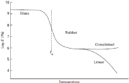
2.4 Tensile and Plastic Behaviors in Polymers
Young’s modulus is dependent on test temperature for amorphous polymers. Close to Tg where the material is in a viscoelastic state, it starts to fall rapidly until the polymer
becomes in a rubbery state (Mullins et al., 2018). Since the thermosets are cross-linked, the elastic modulus remains almost constant when the temperature keeps increasing. Tensile behavior is associated with molecular motions and everything that have an effect on the molecular motion will make changes on its behavior such as the molecular structure, molecular weight, cross-linking density, and temperature (Rudin, 1998; Mullins et al., 2018).
Figure 11: Young’s Modulus-Temperature curve for polymers showing difference between Cross-linked and Linear polymers in the rubbery state (Reprinted from Mullins et al., 2018). In thermosets, shear yielding is most common. If the material does not exhibit an early brittle fracture, it can undergo plastic deformations at high strain levels (Mullins et al., 2018). In glassy polymers, if shear yielding is homogeneously distributed on the vicinity of a crack. The ductile failure will generally occur with the material gaining high toughness (ibid). This happens since a high portion of the fracture energy is absorbed by the plastic deformation. Thus, shear yielding can be a toughening mechanism in polymers (ibid). There are two simple equations that can predict the start of yielding; Von-Mises and Tresca (Hertzberg et al., 2012; Mullins et al., 2018). Von-Mises states that the yield will start when the elastic-shear strain-energy density reaches a critical value.
(𝜎1− 𝜎2)2+ (𝜎1− 𝜎2)2+ (𝜎1− 𝜎2)2= 6𝜏𝑦2 (4) While Tresca suggests that the yield will start when the maximum shear stress on any plane reaches a critical value.
polymers in certain conditions (Mullins et al., 2018). It suggests that yield stresses in uniaxial tension will be equal to yield stresses in uniaxial compression. However, for polymers, the compression yield stresses are usually 15% higher than tensile yield stresses (Landel et al., 1993; Mullins et al., 2018).
Figure 12: Stress-strain behavior of polystyrene under tension and compression (Reprinted from Landel et al., 1993).
2.5 Fatigue Behavior in Polymers
2.5.1 Thermal Fatigue
When applying cyclic stress on a material it initiates microscopic cracks at internal areas where there is stress concentration. Polymers tend to fail at much lower stresses due to fatigue than static loading conditions (Sauer et al., 1980). Early studies of fatigue in polymers have been using unnotched specimen, where it has proved useful in metals. However, in polymers it might raise the question of heating that can lead to failure by thermal melting. There is a critical frequency of cyclic loading where thermal effects need to be considered (Sauer et al., 1980; Ward et al., 2004; Hertzberg et al., 2012). The viscoelasticity of polymers and its poor conductivity of heat makes them more sensitive to temperature than metals to the frequency of alternating loads (Sauer et al., 1980). If isothermal conditions are not met under the loading, hysteretic energy generated during each cycle will be dissipated as heat and it will rise up the temperature of the specimen. This makes it more vulnerable to failure from thermal rapture and melting (Sauer et al., 1980; Hertzberg et al., 2012). The energy lost during the cyclic loading for a given cycle can be given by the following relation (Ferry et al., 1970; as cited in Sauer et al., 1980; Hertzberg et al., 2012):
𝐸̇ = 𝜋𝑓𝐽"(𝑓, 𝑇, 𝜎)𝜎2 (6)
Where f is the frequency, J” is the loss compliance, and σ is the stress. By neglecting heat lost to environment, ∆𝑇̇ will increase with the increase of frequency, stress amplitude, and internal friction (Sauer et al., 1980; Hertzberg et al., 2012). The temperature rise will be retrieved through the following relation (Hertzberg et al., 2012):
∆𝑇̇ = 𝜋𝑓𝐽"(𝑓, 𝑇)𝜎 2
𝜌𝑐𝑝
(7)
Where ∆𝑇̇ is the rate of change of temperature over time, 𝜌 is the density, and Cp is
the specific heat. Many examples of temperature rise in fatigue testing of polymers have been documented. The temperature shows a linear increase with the increase of frequency in unnotched polyethylene (PE) specimens, that increase becomes rapid when increasing the applied alternating stress (Sauer et al., 1977; as cited in Sauer et al., 1980). As for polymethylmethacrylate (PMMA) specimen tested in cyclic bending at 50 Hz the temperature reached values close to 100 C at failure (Oldyrev et al., 1975: as cited in Sauer et al., 1980).
Figure 13: PE specimen temperature-test speed at different stresses (Reprinted from Sauer et al., 1977; as cited in Sauer et al., 1980)
Another interesting observation on the influence of stress amplitude on temperature rise under cyclic load has been observed for polyoxymethylene (POM). For samples tested at constant testing speed, at 22.4 MPa, the temperature rise steadily until reaching thermal failure. However, on stresses below 21.6 MPa the temperature will rise slowly and then stabilizes at the final value (Crawford et al., 1975; as cited in Sauer et al., 1980). This means that one cannot measure the correct stress/cycle values at the exact room temperature as the internal temperature of the specimen will keep rising and is dependent on frequency, stress amplitude, and other material characteristics (Sauer et al., 1980). When the temperature increases, Young’s Modulus decreases, thus increasing the deflections, these deflections produce even more energy that will dissipate as heat with each cycle (Hertzberg et al., 2012).
Figure 14: Temperature-cycle rise for POM at different stresses (Reprinted from Crawford et al., 1975; as cited in Sauer et al., 1980).
In unnotched specimens, temperature increase can be reduced by strain cycling at constant strain rate instead of stress cycling. As in strain cycling there will be lower energy dissipation and no thermal discharge, while in stress cycling it is vise-versa. Unless frequency and stress are kept at lower levels, thermal discharge will occur due to viscoelasticity (ibid). Testing with unnotched specimens does not distinguish between crack initiation and crack propagation when studying the fatigue behavior (Ward et al., 2004). An initial sharp crack can be introduced in order to examine how the crack propagates using fracture mechanics concept (ibid). Hertzberg et al., 2012 concluded that thermal failure comes in the last stages of cyclic life. To prove this a number of experiments have been conducted involved introducing periodic resting times during testing. This method has improved life of the specimen greatly through cooling down temperatures arise from adiabatic heating (ibid). Other methods represented by Hertzberg et al., 2012 to suppress thermal fatigue are limiting stress, decreasing frequency, and increasing the specimen’s surface-to-volume ratio.
2.5.2 Mechanical Fatigue
Test frequency has an influence on the testing process; however, it depends on the viscoelasticity of the polymer in the test temperature (ibid). In materials where thermal effects are not dominant, increasing frequency rates might increase fatigue lifetime. This is due to higher strain rates and tensile modulus. Other reason for the increase is the generation of localized heat at the crack end. This heat has the ability to slow down the crack propagation rate. This has been noticed in PS and PMMA
1975; as cited in Sauer et al., 1980). The stress value at which thermal runaway occurs also depends on the frequency level, In POM it has been found that when lowering the frequency, the thermal runaway starts at higher stress levels. (Crawford et al., 1975 as cited in Sauer et al., 1980).
In cyclic loading, fatigue life decreases with the increase of the mean stress. The change in mean stress also make changes in the fracture surface shape (Sauer et al., 1980). It has been noticed in some materials such as polystyrene (PS), fatigue resistance increases if the mean stress is increased while maintaining a constant maximum stress value (Mukherjee et al., 1971; as cited in Sauer et al., 1980). In purely tensile cycling mode, concentric growth bands are observed in the fracture of many polymers such as PS, PE, and PVC (Sauer et al., 1980). The number of cycles/bands is a function of the stress intensity factor range ∆𝐾. At high values of ∆𝐾 the crack jumps incrementally at each cycle due to fatigue striations (ibid). Polymer structure also plays a role in its fatigue life. Crystalline polymers have higher fatigue resistance than amorphous polymers due to its two-phase structure and its ability to absorb fracture energy (ibid). Fatigue in crystalline polymers is preceded by formation of a damage zone at the crack tip, but in glassy amorphous polymers it is preceded by crazing (ibid). It has been also noticed that the degree of cross-linking has a positive effect on crack propagation rates and toughness, hence increasing crosslinking decreased crack propagation rates. This is due to increase in molecular weight and increased capacity for plastic deformation (ibid).
3 Theory
3.1 Linear Elasticity and Stress-Strain Relations
Stress and strain are classically defined by the scope of small deformations. The relationships of each point fixed on the material body will be assumed linear (Bergström, 2015). The stress component can be illustrated as follows:
●
Figure 15: Normal and shear stress components (Reprinted from EngApplets 2019). where the outwards pointing arrows normal on the faces of the on an infinitesimal cubic body are the normal stresses and the arrows parallel to the face of the body are representing shear stress (Ward et al., 2004, Bergström, 2015). Thus, the components of stress are defined by nine elements that form the stress tensor:
𝜎𝑖𝑗 = [
𝜎𝑥𝑥 𝜎𝑥𝑦 𝜎𝑥𝑧 𝜎𝑥𝑦 𝜎𝑦𝑦 𝜎𝑦𝑧 𝜎𝑥𝑧 𝜎𝑦𝑧 𝜎𝑧𝑧
] (8)
The first subscript of the stress refers to the direction normal on the surface of the body and the second refers to the direction of the stress (ibid). Assuming that the cube is in an equilibrium state the stresses will have the following equalities:
𝜎𝑥𝑦 = 𝜎𝑦𝑥, 𝜎𝑥𝑧= 𝜎𝑧𝑥, 𝜎𝑦𝑧 = 𝜎𝑧𝑦 (9) The stress state of a body can be known if six stress components are identified (Ward et al., 2004). In the case of strain, it is mainly categorized into two types. The first type is extensional strain which is the change in length in the pulling force direction. The second type is simple shear strain which is the displacement of parallel planes as shown in the figure below (ibid).
Figure 16: Representation of extensional strain (left) and simple shear strain (right) (Reprinted from Ward et al., 2004).
The angle 𝜃 represents the displacement between the two parallel planes divided by the perpendicular distance between the same planes (ibid). Strain is a unitless variable and sometimes it is denoted in percentages. Similar to stress, the components of strain can be given by the strain tensor (ibid):
𝜀𝑖𝑗= [ 𝜕𝑢𝑥 𝜕𝑥 1 2( 𝜕𝑢𝑦 𝜕𝑥 + 𝜕𝑢𝑥 𝜕𝑦) 1 2( 𝜕𝑤 𝜕𝑥 + 𝜕𝑢𝑥 𝜕𝑧) 1 2( 𝜕𝑢𝑦 𝜕𝑥 + 𝜕𝑢𝑥 𝜕𝑦) 𝜕𝑢𝑦 𝜕𝑦 1 2( 𝜕𝑢𝑦 𝜕𝑧 + 𝜕𝑢𝑧 𝜕𝑦) 1 2( 𝜕𝑢𝑧 𝜕𝑥 + 𝜕𝑢𝑥 𝜕𝑧) 1 2( 𝜕𝑢𝑦 𝜕𝑧 + 𝜕𝑢𝑧 𝜕𝑦) 𝜕𝑢𝑧 𝜕𝑧 ] (10)
In the most evident case, it is assumed that stress and engineering strain are linearly related to each other. Each of the six components of stress are related to six independent component of strain (ibid), as shown in the expression of generalized Hooke’s law for both isotropic and anisotropic solids:
𝜎𝑥𝑥 = 𝑎𝜀𝑥𝑥 + 𝑏𝜀𝑦𝑦 + 𝑐𝜀𝑧𝑧 + 𝑑𝜀𝑥𝑧 . . . 𝑒𝑡𝑐 (11) For an isotropic material, the stress is proportional to strain and is unaffected by the direction or orientation of the body (Ward et al., 2004; Bergström, 2015). Considering one dimension, e.g. strains in the X direction, we have:
𝜎𝑥𝑥 = 𝐸𝜀𝑥𝑥 (12)
where E is called the Young’s modulus or the modulus of elasticity. These equations can be developed into the following form for strains in the y and z direction:
𝜀𝑥𝑥 = −𝑣
𝐸 𝜎𝑥𝑥, 𝜀𝑧𝑧 = −𝑣
𝐸 𝜎𝑥𝑥
(13)
Where v is Poisson’s ratio is the relation between the contraction strain 𝜀𝑦𝑦 to the extensional strain 𝜀𝑥𝑥 (ibid). similarly for the other two direction, we can obtain the following stress-strain relations:
𝜀𝑥𝑥 = 1 𝐸 𝜎𝑥𝑥− 𝑣 𝐸(𝜎𝑦𝑦+ 𝜎𝑧𝑧) 𝜀𝑦𝑦 = 1 𝐸 𝜎𝑦𝑦− 𝑣 𝐸(𝜎𝑥𝑥+ 𝜎𝑧𝑧) 𝜀𝑧𝑧 = 1 𝐸 𝜎𝑧𝑧− 𝑣 𝐸(𝜎𝑥𝑥+ 𝜎𝑦𝑦) 𝜀𝑥𝑧 = 1 𝐺 𝜎𝑥𝑧, 𝜀𝑦𝑧 = 1 𝐺 𝜎𝑦𝑧, 𝜀𝑥𝑦 = 1 𝐺 𝜎𝑥𝑦 𝐺 = 𝐸 2(1 + 𝑣) (14) (15) (16) (17) (18)
Where G is the shear modulus which is the constant in the relation between shear stress and its corresponding shear strain.
Young’s Modulus can be influenced by temperature in polymers. The polymer structure plays a role in determining the modulus as its molecules are constructed with covalent bonds and the strength of these can differ from one type to another (Hertzberg et al., 2012). In highly cross-linked rigid thermosets, where Tg tend to be
high, a change in the molecular structure is difficult to accomplish, thus the material can have a relatively high Young’s modulus (ibid).
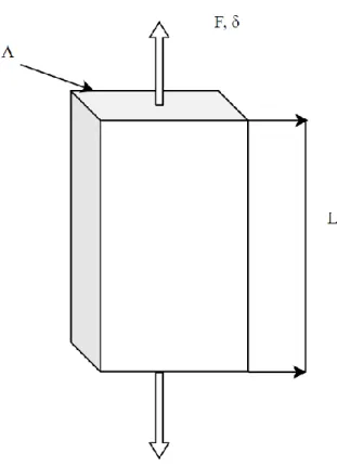
To define stress and strain deformations there are multiple approaches. The classical approach is through uniaxial deformation where a force is acting perpendicularly to the cross-sectional area of the tested material specimen as shown in figure 17 (Bergström, 2015). The stress and strain will be calculated as follows:
𝜎 = 𝐹 𝐴 𝜀 = ẟ 𝐿 (19) (20)
Where 𝜎 is the stress, F is the force, A is the cross-sectional area of the body. 𝜀 is the perpendicular strain, ẟ is the displacement, and L is the original length of the body. In the small strain theory, it is assumed that the changes in dimensions during loading are so small that they can be represented using linear representation and there is only one stress and one strain to measure (ibid).
Figure 17: Illustration of uniaxial loading
It is important to make a distinction between engineering strain and true stress-strain. The terms used extensively in engineering practice are defined as follows (Hertzberg et al., 2012): 𝜎𝑒𝑛𝑔 = 𝐹 𝐴𝑜 𝜀𝑒𝑛𝑔 = ẟ 𝐿𝑜 (21) (22)
Where F is the load, 𝐴𝑜is the initial cross-sectional area, ẟ is the displacement, and 𝐿𝑜 is the initial length While true stress and strain can be defined as:
𝜎𝑡𝑟𝑢𝑒 = 𝐹 𝐴𝑖 𝜀𝑡𝑟𝑢𝑒 = 𝑙𝑛 𝑙𝑓 𝐿𝑜 (23) (24)
Where 𝐴𝑖 is the instantaneous cross-sectional area and 𝑙𝑓 is the final length.
3.2 Cyclic Stresses
Cyclic stresses (or fatigue stresses) are common in engineering problems, for example, alternating stresses accompanying a rotating shaft, pressurizing and depressurizing cycles of an aircraft, and load fluctuations affecting wings (Hertzberg et al., 2012). According to Wright, 2001, fatigue is the second most common cause of failure and account to 15% of failures in plastics. The design engineer must be aware of the risk of cyclic loads, which are common in vehicles, that might cause failure to the product (ibid). A general fatigue failure involves initiation of a crack that keep propagates with each cycle until the material fails and fractures. This happens within intermediate values of stress that falls between ¼ and ½ of the tensile or ultimate stress (Sauer et al., 1980). Cracks can be classified into two categories; small cracks that interacts with the microstructure of the material and are shear driven, and large cracks that are almost insensitive to the microstructure of the material and are tension driven (Ekberg, 1998). Small cracks tend to propagate faster than larger ones. However, crack closure phenomena is asserted in large cracks. It is one of the causes of crack arrestment where fatigue crack growth rate will be decreased due to residual stresses (ibid).
Figure 18: Stages of crack initiation and propagation (Reprinted from Ekberg, 1998). Studies of fatigue fracture in polymers are usually made by fracture mechanics experiments (ibid). In notched specimens, the stress intensity factor can be calculated through the following relations:
𝐾 = 𝑌𝜎√𝑎 (25)
Where K is the intensity factor, Y is the geometrical value (√𝜋 for a central crack length of 2a), and 𝜎 is the stress (ibid). These tests are usually performed with a stress ratio of 0.1 where R = min stress/max stress (ibid). In order to study the service life of a material that is going to be used in designing a new part, the integration of the Paris equation can be used with the start and end of the flaw as integration limits (Ekberg, 1998; Hertzberg et al., 2012, Ward et al., 2004):
𝑑𝑎
𝑑𝑁= 𝐴∆𝐾
𝑚 (26)
Where A and m are material properties that are also a function of temperature, ∆𝐾 is the range of the stress intensity factor (Sauer et al., 1980). Stress variables can be defined as follows (Hertzberg et al., 2012):
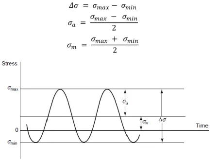
𝛥𝜎 = 𝜎𝑚𝑎𝑥− 𝜎𝑚𝑖𝑛 𝜎𝑎 = 𝜎𝑚𝑎𝑥 − 𝜎𝑚𝑖𝑛 2 𝜎𝑚 = 𝜎𝑚𝑎𝑥 + 𝜎𝑚𝑖𝑛 2 (27) (28) (29)
Figure 19: Cyclic stress parameters (Reprinted from Hertzberg et al., 2012). Generally, a fatigue test involves a mean stress 𝜎𝑚where a sinusoidal cycle is imposed on it (Roylance, 2001). This cycle can be asserted in terms of alternating stress and stress ratio R where:
𝑅 = 𝜎𝑚𝑖𝑛 𝜎𝑚𝑎𝑥
(30)
For fully reversed loading, a ratio of R = -1, 𝜎𝑚 = 0 and the sinusoidal stress have a tension-compression cycle. For a tension-tension cycle, a value of R = 0.1 is used. This ratio is often used in aircraft component testing (ibid), it corresponds to a value of
𝜎𝑚𝑖𝑛
= 0.1 ∗ 𝜎
𝑚𝑎𝑥 (31)S-N diagrams are the standard method to describe and calculate fatigue life. It has been used in the early studies of polymer fatigue as this method has already proved practical with metals. The Y axis usually denotes the stress amplitude 𝜎𝑎 and the X axis number of cycles to failure N. They are commonly plotted with logarithmic (log-log) axes. SN curves fitted to data derived from experimental fatigue tests are the best way to describe fatigue strength to a great degree (Ward et al., 2004; Hertzberg et al., 2012; Pedersen, 2018). It has been observed from a number of tests that there is a linear relation between the intermediate values of log of stress and the log of cycles to failure (ibid). As the stress range decreases, the S-N curves flats and the limiting
stress will be called endurance limit where no fatigue will happen below that stress (ibid).
Figure 20: Typical S-N curve (Reprinted from Hertzberg et al., 2012).
A major aspect the when conducting tests on polymers to be aware of the influence of adiabatic heating that can generate when doing fatigue tests in polymers. Meaning that there will be not enough time for heat to dissipate thus increasing the temperature of the polymer that can lead to thermal fatigue (Sauer et al., 1980; Ward et al., 2004; Hertzberg et al., 2012).
3.3 Viscoelastic Behavior of Polymers
There are two constitutive models that can describe the mechanical properties of ideal materials (Ottosen et al., 2005; Malkin et al., 2012):
1. Newton’s law of Liquids:
𝜎𝑣= 𝜂𝜀̇𝑣 (32)
2. Hooke’s law of Solids:
𝜎
𝑒= 𝐸𝜀
𝑒 (33)Where in the first law
𝜀
𝑒is rate of change in shear strain, 𝜎𝑣 is the shear stress, and η is the viscosity. In the second law ε is the strain, 𝜎𝑒 is the tensile stress, and E is the Young’s modulus. Polymers have an interesting feature where it shows both behaviors and act as an elastic solid or a viscous liquid depending on temperature and experiment time, this kind of behavior is called viscoelasticity (Ward et al., 2004). Newton’s law of viscosity can be translated to the following equation (ibid):𝜎 = 𝜂𝜕𝑉𝑥 𝜕𝑦
(33)
Where 𝑉𝑥 is the velocity and y is the direction of the velocity gradient. Since velocity is the change of displacement with time, in an xy-plane we get the following equation (ibid): 𝜎𝑥𝑦= 𝜂 [ 𝜕 𝜕𝑦( 𝜕𝑢𝑥 𝜕𝑡) + 𝜕 𝜕𝑥( 𝜕𝑢𝑦 𝜕𝑡 )] = 𝜂 𝜕 𝜕𝑡( 𝜕𝑢𝑥 𝜕𝑦 + 𝜕𝑢𝑦 𝜕𝑥) (34)
Where 𝑢𝑥 and 𝑢𝑦 are the displacement in x and y directions respectively, and t is time. It can also be written as (ibid):
𝜎𝑥𝑦 = 𝜂 𝜕𝜀𝑥𝑦
𝜕𝑡
(35)
Where 𝜀𝑥𝑦 is the shear strain. In Hooke’s law the stress is linearly related to the strain, however, in the above equation it is linearly related to the change in strain over time (ibid). For the elastic behavior the shear modulus will be used instead of the elastic modulus in order to build a simple constitutive relation for the viscoelastic behavior. The simplest possible form of linear viscoelasticity is (ibid):
𝜎𝑥𝑦 = (𝜎𝑥𝑦)𝐸+ (𝜎𝑥𝑦)𝑉= 𝐺ε𝑥𝑦+ 𝜂 𝜕ε𝑥𝑦
𝜕𝑡 (36)
This formulation is called the Kelvin-Voigt model. However, there are multiple possible formulation of viscoelastic behavior to unite those constitutive relations (ibid). For better understanding these relations, it can be illustrated by simple mechanical models. Viscous behavior is modeled as a dashpot (damper) and the elastic behavior is modeled after a spring (Bergström, 2015; Malkin et al., 2012; Ward et al., 2004). The use of these models is very instructive and it increases our capacity to understand material behavior in different stress-strain conditions (Malkin et al., 2012).
Figure 21: The fundamental mechanical models representing viscoelasticity, on the top is the Kelvin-Voigt model and on the bottom is the Maxwell model.
As illustrated in figure 21, the Kelvin-Voigt model consists of a spring with a spring modulus E in parallel with a dashpot with viscosity 𝜂. If constant stress is applied, the spring do not deform instantly as it is going to be retarded by the dashpot as the stress is shared by both components in the parallel connection. After a period of time dependent on the viscosity 𝜂, the spring will be fully deformed. However, when removing the stress, the process will be reversed and it will return to its initial unstretched state (Ward et al., 2004). The Maxwell model represent a spring and a dashpot series connection. When applying constant displacement, it will immediately deform the spring. As time proceeds, the deformation will be transferred to the dashpot element and the spring will be released (Malkin et al., 2012; Ward et al., 2004). Both Maxwell and Kelvin-Voigt models predict the behavior of different materials as Maxwell is suited for liquids and Kelvin-Voigt for solids. These models can be combined in parallel and in series together to predict behavior such as the Zener model or Burgers model which is a quantitative model of behavior of polymers (Malkin et al., 2012; Ottosen et al., 2005; Moczo et al., 2006). In general, the series connection makes the stress equal and strain additive, while the parallel connection makes the strain equal and the stress additive. From these rules mathematical formulations can be drawn for different models (Moczo et al., 2006).
Viscoelastic processes can be determined from simple creep and stress relaxation experiments. Creep is the time-dependent deformation that occurs while applying a constant stress. On the contrary, stress relaxation is the time-dependent change in stress when applying a constant strain (Ward et al., 2004). Wright, 2001, suggests that 8% of failures in polymers are due to creep or stress relaxation behaviors. This is due to a number of reasons including delayed buckling or decline in mechanical jointing forces. Poor design decisions can also lead to creep/stress relaxation failures. Data related to such behavior are limited or not sufficient for the design engineer to make proper design decisions. Creep and relaxation behavior are also heavily dependent on the temperature. The design engineer needs to be informed about how temperature change influences the viscoelastic behaviors (ibid). The Kelvin-Voigt model is more suitable for modeling the creep behavior as first approximation. While the Maxwell model has more value in modeling a stress relaxation behavior to a first approximation
Figure 22: Time dependent behavior of (a) stress-relaxation, (b) creep (Reprinted from Ashter, 2013).
One of the simplest and most used ways to express the viscoelastic behavior of polymers is through linear viscoelasticity. A fundamental rule in linear viscoelasticity is to consider “Each loading step makes an independent contribution to the final state.” which can also be called Boltzmann superposition (Bergström, 2015). Thus, strain history will be considered as a sum of infinitesimal strains:
𝜀(𝑡) = ∑ ∆𝜀𝑖𝐻(𝑡 − 𝜏𝑖) ∞
𝑖=1
(37)
When applying this to stress we obtain the stress response: 𝜎(𝑡) = ∑ ∆𝜀𝑖𝐸𝑅(𝑡 − 𝜏𝑖)
∞
𝑖=1
(38)
In cyclic loading, e.g. sinusoidal strain, there will be a lag between applied strain and stress response. The stress response is also sinusoidal but is shifted with a phase angle δ (ibid). In case of applying a sinusoidal strain:
𝜀(𝑡) = 𝜀𝑚+ 𝜀𝑎sin (𝜔𝑡) (39)
Where, 𝜀𝑚 is the mean strain, 𝜀𝑎 is the strain amplitude and ω is the angular frequency. The following stress response is obtained:
𝜎(𝑡) = 𝜎𝑚+ 𝜎𝑎sin (𝜔𝑡 + 𝛿) (40) This can be re written in terms of phase difference with the applied strain (ibid):
𝜎(𝑡) = 𝜎𝑚+ 𝜎𝑎cos(𝛿) sin(𝜔𝑡) + 𝜎𝑎sin(𝛿) cos(𝜔𝑡) (41) Let us define the storage modulus E’ and loss modulus E”. E’ represents the elastic response that represents the energy stored in the specimen and is in phase with the
strain, while E” is the viscous response that represents the energy dissipated out of the specimen and is lagging 90o from the strain. The latter is also connected to the
heat dissipation during cyclic loading (Ward et al., 2004, Bergström, 2015). The stress response can be given by:
𝜎(𝑡) ≡ 𝜎𝑚+ 𝜀𝑎𝐸′sin(𝜔𝑡) + 𝜀𝑎𝐸" cos(𝜔𝑡) (42) By defining a complex modulus E* we can get the following relations:
𝐸′ = 𝐸∗cos (𝛿) 𝐸" = 𝐸∗sin (𝛿) (43) (44) Given (Bergström, 2015): 𝐸∗=𝜎𝑎 𝜀𝑎 (45)
The complex modulus is also treated as a complex number, hence the name, as shown in the relation:
𝐸 ∗= 𝐸’ + 𝑖𝐸” (46)
Where i is the imaginary unit (Lakes, 2019, Bergström, 2015). The ratio between the loss to storage modulus is called the damping ratio, it is given as:
tan 𝛿 = 𝐸" 𝐸′
(47)
Thus, when the damping ratio increase, the material tends to dissipate energy, while if it decreases, it tends to store the energy and becomes closer to a purely elastic material (Menard et al., 2006). The phase difference δ can be calculated through the following relation:
𝛿 = (2𝜋 𝛥𝑡 T )
(48)
Where T is the time needed for one cycle of load. Δt is the time difference between the stress and strain curves (Lakes, 2019).
4 Methods
This study will be carried out using a mix of qualitative and quantitative approaches. The data gathered from the tests are analyzed by statistical models, i.e. this approach will be qualitative. However, an investigation of the failed specimens will be carried out using a microscope. This observation method is qualitative and its results will be correlated with the quantitative results in the final analysis.
4.1 Determination of Tensile Properties
4.1.1 Uniaxial Tension Testing
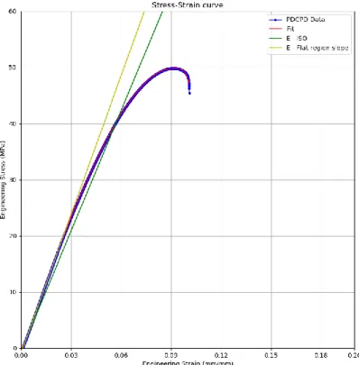
In order to determine the tensile properties of the plastic material the methods and guidelines specified in ISO 527-1:2018 have been used. It is used to investigate the tensile properties of specimens such as the relationship between stress and strain, tensile strength, and Young’s Modulus (ISO 527-1:2018). These guidelines are suitable for rigid thermosets including filled and reinforced composites (ibid). A dog-bone shaped specimen is used for uniaxial tensile tests. This specimen design is adequate for creating a uniform uniaxial deformation and stress state in the gauge of the specimen. It also reduces the stress concentrations in the parts that are close to the grips of the testing machine (Bergström, 2015). The guidelines for the design of test specimens for plastic materials defined at ISO 20753:2018. One drawback of the dog-bone shape of test specimens is the necking phenomena. It creates an inhomogeneous deformation in the specimen which makes it difficult to measure the actual stress-strain response (Bergström, 2015). One way to solve this issue is through using a digital image correlation (DIC) system (ibid). The results of this test can be plotted as a stress-strain plot, the elastic modulus can be calculated by finding the slope of the flat elastic region (McKeen, 2016) as shown in figure 24 below:
4.1.2 Creep Testing
Creep testing guidelines ISO 899-1:2017 shall be followed. Creep is carried out by applying constant load on a specimen for a certain period of time while monitoring the change in its strain levels. It can be sensitive to the geometry and service history of the tested material during testing. For precise results it is desirable that the testing is done over a broad range of stresses, times, and ambient conditions (ibid). The specimens are to be loaded smoothly with the desired load being reached in 1-5 seconds. The results shall be later presented in creep curves showing strain against time and creep modulus against time (ibid).
4.1.3 Digital Image Correlation (DIC)
Digital image correlation is an image processing method that uses recorded images to capture and analyses measurement data (Schreier et al., 2009). This method is applied to acquire high resolution strain data by recording images of a loaded, patterned specimen. A speckle pattern is suitable for DIC strain measurements where the DIC system can locate the random dots and capture its deformation behavior (Cintrón et al., 2008). The DIC measurements are dependent on a number of variables which are the image resolution, pixels, the geometry of the specimen, focal length of the camera, distance between the recorded specimen and the camera, and the speckle pattern applied on the specimen (ibid). DIC measurements are similar to those obtained from direct strain gauges attached to the tested specimen. However, it provides advantages in terms of relative ease, less preparation times and data analysis (Hensley et al., 2017). For this research, GOM ARAMIS DIC system has been used to measure strains during tensile tests. The system is equipped with two 75mm lens cameras and has been calibrated according to the test settings. Later the data was analyzed using GOM Correlate 2018 software.
4.2 Mechanical and Thermal Fatigue
4.2.1 Cyclic Tension Test
The guidelines specified in the standard ASTM D7791 − 17 covers the determination of dynamic fatigue properties of plastics in uniaxial loading conditions. Tension or compression loading can be used in order to determine these properties. For tension loading condition, a specimen of a rectangular cross-section is gripped by its ends and pulled in opposite directions equally then released back to its initial condition (ASTM D7791 − 17). The load will be cyclic and at least four stress levels will be tested. The test frequency is uniform and it ranges from 1-25 Hz. After fracture it can be determined at which number of cycles the specimen has failed. For fatigue analysis, a cyclic stress level shall be applied and a S-N curve will be constructed denoting the stress level versus the number of cycles to failure.
4.2.2 Thermography
A high-performance IR camera (FLIR A65) is used to capture thermal activity in the specimen during cyclic loading testing. The camera has a focal length of 13 mm and IR resolution of 640x512 pixels with a spectral range of 7.5–13 µm. A software is included to capture the data out of the camera and record it into a picture, video, or spreadsheet format. Thermography is capable of opening a wide range of application in thermomechanical processes such as mechanical damages and phase transformations of materials and its inner structural state. The rate of temperature increase at crack tips during fatigue can be a good indicator to predict the final failure state (Yang et al., 2004).