Southern Swedish Forest Research Centre
Thinning response to weather
variations in Norway spruce
Gallringsrespons på vädervariationer hos gran
Thinning response to weather variations in Norway spruce
Gallringsrespons på vädervariationer hos gran
Erika Alm
Supervisor: Urban Nilsson, SLU Southern Swedish Forest Research Centre Assistant supervisor: Igor Drobyshev, SLU Southern Swedish Forest Research Centre Examiner: Eric Agestam, SLU Southern Swedish Forest Research Centre
Credits: 30 credits
Level: Advanced level, A2E
Course title: Master thesis in Forest Science
Course code: EX0928
Programme/education: Euroforester master’s programme
Course coordinating department: Southern Swedish Forest Research Centre
Place of publication: Alnarp
Year of publication: 2019
Online publication: https://stud.epsilon.slu.se
I would like to thank my supervisor Urban Nilsson his guidance, and my as-sistant supervisor Igor Drobyshev, especially for his help to date my samples correctly. A special thanks to Guilherme Pinto who helped me with the sam-ple preparation and to Emma Holmström for always answering my questions about R studio.
Climate change is likely to affect the prerequisites for forest management. Therefore, it is imperative to investigate how silviculture practices can be adjusted to changing conditions. Norway spruce (Picea abies) is one of the most common species in the Swedish forests, with high economic and ecological values. The species is relatively sensitive to drought, and climate change is likely to entail more frequent drought periods. Thinning is considered to decrease the competition of resources between the trees in a forest stand. Thus, it might be possible to decrease the negative effect of drought by conducting thinnings. The purpose of this study was to investigate if weather conditions affect the individual tree growth response to thinning in spruce stands, and if some thinning methods made the stands more resilient to weather con-ditions. The analysis was conducted with tree cores sampled from the thinning and fertilization experiments, a large field experiment with sites all over the country. Four sites in southern Sweden were selected. One control treatment and two thinning meth-ods were chosen from each site: one heavy thinning (treatment c) and 2 – 6 thinnings from below (treatment A/E). The ring widths were measured in a dendrochronology laboratory.
The results showed a clear difference in growth between the heavy thin-ning and the other treatments. After a heavy thinthin-ning had been conducted, the Basal area increment of the remaining trees increased. The same pattern could to some ex-tent be observed for the other treatments as well, however the increase was not as great. For the years where the Basal Area Increment was unusually low in the control plot, the treatments seemed to do slightly better, however the result was not signifi-cant. The weather-growth relationship was analysed with the R package treeclim, however precipitation and growth only seemed to correlate before thinning for the A/E treatment. The sample used in this study was relatively small and larger experi-ments including more samples and perhaps other tree species could give a better pic-ture of how Norway spruce should be managed in the fupic-ture. Thinning is a powerful forest management tool that could play a key role when adapting forests to climate change. Thus, the application of thinnings in forest management needs to be further investigated.
Keywords: Thinning, Climate change, Dendrochronology
Abstract
Det är troligt att förutsättningarna för skogsbruk kommer påverkas av klimatföränd-ringarna. Det behövs mer forskning kring samspelet mellan skogsskötsel och klimat. Gran (Picea abies) är ett av de vanligaste trädslagen i Sverige, och har både ekono-miska och ekonoekono-miska värden knutna till sig. Arten är relativt känslig mot torka, ett fenomen som troligtvis kommer bli alltmer frekvent i och med klimatförändringarna. Gallring är ett sätt att minska konkurrensen av resurser i ett skogsbestånd, och skulle därmed kunna bidra till att sänka de negativa effekterna torka kan innebära. Syftet med den här studien var att undersöka om klimatvariationer påverkar tillväxtrespon-sen hos individuella träds gallringsrespons, samt om vissa gallringsmetoder leder till bättre resiliens mot varierande väderförhållanden. Analysen utfördes med borrkärnor som samlats in från gallrings- och gödselförsöken, ett stort experiment med ytor i hela Sverige. Data kom från fyra olika ytor i södra Sverige. Två gallringsmetoder från varje yta var representerade: En intensiv gallring (behandling C) och en där par-cellerna gallrades 2 – 6 gånger innan avverkning (behandling A/E). från varje yta inkluderades en obehandlad kontrollparcell. Borrkärnorna preparerades och mättes i ett laboratorium innan data importerades till R studio.
Resultaten indikerade en tydlig skillnad i tillväxt mellan de olika parcel-lerna. En stor gallring resulterade i en kraftig ökning i grundytetillväxten för de kvar-varande träden. Samma trend kunde identifieras för behandling A/E, men ökningen var då inte lika markant. De år kontrollens grundytetillväxt var lägre än vanligt ver-kade behandlingarna klara sig något bättre, men ingen signifikant skillnad gick att utläsa. När sambandet mellan nederbörd och tillväxt analyserades med hjälp av pa-ketet treeclim i R studio gick det endast att se ett samband mellan dessa variabler före gallring i behandling A/E. Urvalet av data som användes var relativt litet vilket kan ha påverkat resultatet. En större studie med mer data, och kanske även fler trädslag, skulle kunna ge en bättre bild av hur gallring bäst ska utföras för att skapa granskogar som är tåliga mot torka. Gallring kan spela en nyckelroll i att anpassa skogsbestånd till klimatförändringarna, det är därför vitalt att låta gallring stå i fokus även i framtida studier som fokuserar på skog och klimat.
Nyckelord: Gallring, Klimatförändringar, Dendrokronologi.
Sammanfattning
Acknowledgements 2 Abstract 3 Sammanfattning 4 List of tables 7 List of figures 8 1 Introduction 11
1.1 Forest management in Sweden: Where are we heading? 11 1.2 Climate change and Norway spruce 12 1.3 Thinning in Norway spruce stands 13 1.3.1 The thinning and fertilization experiments in Sweden 14 1.4 A dendrochronological approach to analyse tree response to thinnings 14 1.5 Aim, delimitations and research questions 15
1.5.1 Delimitation 15
1.5.2 Research questions 15
1.5.3 Hypotheses 15
2 Material and methods 16
2.1 Study sites 16
2.1.1 Thinning methods 17 2.1.2 Experimental design 18
2.2 Sample preparation 18
2.2.1 Tree core sampling 18 2.2.2 Laboratory work 18
2.3 Data analysis 20
2.3.1 Basal Area Increment 20
2.3.2 DplR package 20
2.3.3 Treeclim package 21
2.3.4 Weather data 21
3 Results 22
3.1 Basal area increment 22
3.2 Comparison of years with high BAI in control plot 24
3.3 Growth and weather analysis 27 3.2.1 Treeclim analysis 28
4 Discussion 30
4.1 Basal Area Increment 30 4.2 Growth and weather analysis 31
4.3 Site selection 31
4.4 Sample quality and sample depth 32 4.5 Scientific importance of the project 32 4.6 Further research and recommendations 33
5 Conclusion 34
Table 1. Sites, site coordinates, plots, treatments, number of samples and thinning
years for all sites. 19
Table 2: Sites, site coordinates, plots, treatments, number of samples, site index and
thinning years for all sites included in the study. 19 Table 3: Extreme years in BAI for the control plots when the growth was unusually low
and how they correlated with the treatments. If they reacted the same, the years received the number “0”. If they react-ed differently, the years received
the number “1”. 27
Table 4: Extreme years in BAI for the control plots when the growth was unusually
high and how they correlated with the treatments. If they reacted the same, the years received the number “0”. If they reacted differently, the years
re-ceived the number “1”. 28
Figure 1: Map showing the location of the sites. Data from Statistiska centralbyrån
(SCB). 18
Figure 2: Measuring tree rings in Coorecorder. 21
Figure 3: Sample depth of all sites combined, illustrated with the grey area in the
graph. The red line in the graph is the fitted spline function. The black line represents the average ring width index (RWI). 21
Figure 4- 8: Precipitation index for each site, starting from 1958 and continuing until
the year when the cores were extracted. 23
Figure 9 - 13: BAI (cm2/year) for each treatment on each site. The control treatment
is the green line, the red line treatment C and the orange treatment A/E. The vertical, dotted lines mark the thinning years. The red line marks thinning years for treatment C, and the orange lines mark the tinning years for treat-ment A/E. The purple dotted lines mark years when both treattreat-ment C and
A/E were thinned. 25
Figure 14- 17: Control treatment for each site with red dotted lines marking the
ex-tremely low BAI chosen for the analysis of extreme years, and black dotted lines for the extremely high BAI. 26
Figure 15 – 19: Ring width indices and summer precipitation index for each treatment
on each site. The control treatment is the green line, the red line treatment C and the orange treatment A/E. The blue, dotted line is the summer
precipita-tion index. 29
Figure 20 and 21: Treatment A/E before thinning. All years before thinning are
aggre-gated and their correlation with the weather conditions is tested using a sim-ple Pearson correlation. The graphs show the correlations between precipi-tation and growth over time as primary variable and mean temperature and growth over time as the secondary variable. The diagram to the left shows the correlations for the same period but in the in the control plots. 30
Figure 22 and 23: Treatment A/E after thinning. All years after thinning are aggregated
and their correlation with the weather conditions is tested using a simple Pearson correlation. The graphs show the correlations between precipitation and growth over time as primary variable and mean temperature and growth over time as the secondary variable. The diagram to the left shows the cor-relations for the same period but in the in the control plots. 30
Figure 24 and 25: Treatment C before thinning. All years before thinning are
aggre-gated and their correlation with the weather conditions is tested using a sim-ple Pearson correlation. The graphs show the correlations between precipi-tation and growth over time as primary variable and mean temperature and growth over time as the secondary variable. The diagram to the left shows the correlations for the same period but in the in the control plots. 31
Figure 26 and 27: Treatment C after thinning. All years after thinning are aggregated
and their correlation with the weather conditions is tested using a simple Pearson correlation. The graphs show the correlations between precipitation and growth over time as primary variable and mean temperature and growth over time as the secondary variable. The diagram to the left shows the cor-relations for the same period but in the in the control plots. 31
1.1 Forest management in Sweden: Where are we
heading?
Climate change is likely to affect the prerequisites for forest management. The In-tergovernmental Panel of Climate Change (IPCC) states in their report from 2018 that “High-latitude tundra and boreal forests are particularly at risk of climate change-induced degradation…” (IPCC, 2018). Climate change is, for example, ex-pected to entail longer and warmer growing seasons, and to increase the overall forest productivity (Suvanto, 2016). However, climate models are also suggesting longer and more severe periods of drought, increased risk for storm damage and pest and insect outbreaks (Hänninen, 2016). It remains to demonstrate how augmented concentrations of CO2 will affect the trees or to what extent increased temperatures will affect the frequency of insect and pest outbreaks (Hänninen, 2016). As stated by Hänninen et al (2011), climate change adaptation will have to include reassess-ment of the contemporary ways to conduct silvicultural practices.
Boreal forests are the largest biome in the world, containing around 30 % of the total forest area and more freshwater than any other biome in the world (Gauthier, 2015). Ideas of afforestation and substitution of fossil fuel products with bioenergy and bioproducts are gaining more and more ground as solutions to many climate-related problems (Beland-Lindahl et al, 2015). However, the subject is troversial. A conflict in Sweden concerning how forests should be used to best con-tribute to sustainable development has arisen, primarily since the revision of the Forestry Act (Beland-Lindahl et al, 2015). The opinions about how Sweden should use its forest resources to build a sustainable society are many and diverse. How-ever, it is evident that resilient forests are key to well-functioning ecosystems and carbon sequestration. To conduct research aiming for efficient use of these resources
is one important approach to adapt forests to climate change. Developing and cus-tomizing thinning strategies are one example of such research.
1.2 Climate change and Norway spruce
Before humans started to influence the species composition in forests some thou-sand years ago, conifer forests mainly dominated the boreal zone whereas southern Sweden contained a more varied forest (Götmark et al., 2005). However, due to the production-focused forestry conducted in Sweden through the 20th century, Norway spruce is now a common species in southern Sweden (Lagergren & Jönsson, 2017).
Since Norway spruce is a species with high economic and ecological value, it is important to investigate how to create the best possible conditions for it to grow. Most of Sweden’s Norway spruce stands are today found in the south of the country. It is widely accepted that the climate in the north is too harsh for the species to produce high timber volumes (Bergh, 2005). This has primarily been con-nected to the difference in temperature, however it could also be concon-nected to the abundance of nutrients in the soil and water supply. Bergh et al (2005) also con-cluded that water abundance in general does not pose problems for forest growth, however water deficit might have a negative effect on the growth in southern Swe-den. It has also been suggested that Norway spruce is more susceptible to drought than Scots pine, another dominant conifer species in Sweden (Heiskanen et al, 2002., Zang et al, 2012).
Compared to deciduous trees, conifer trees and Norway spruce in particu-lar are considered more susceptible to storm damage. Norway spruce is a sensitive species to storms, pests and insect outbreaks, and these events are supposed to in-crease with climate change (Lagergren & Jönsson, 2017). Hence, the need for resil-ient forests is growing and there are different views on how they can be created. One approach is to shorten the rotation periods and thus shorten the time under which the trees are exposed to risk for storm damage (Nilsson, 2013). Responses to climate change vary not only between tree species, the response can also depend on the provenances, since trees will adapt to the specific site conditions where they grow (Suvanto, 2016). Thus, environmental conditions can be an important factor when it comes to growth response to treatments and needs to be further investigated (Suvanto, 2016).
Despite the sensitivity to climate change, Norway spruce is still the most commonly planted tree species in southern Sweden. According to Lodin et al (2017), the main reasons are the profit focus in Swedish forestry, the expertise and knowledge that can be found concerning the species in combination with restraining browsing pressure and present soil conditions.
1.3 Thinning in Norway spruce stands
Thinnings are a common method to increase radial growth in Norway spruce stands. A thinning is when trees are felled to increase the quality and economic profit of the remaining trees (Agestam, 2009). The most common way to conduct thinnings in Sweden is to do two – three thinnings from below before the final harvest, meaning the supressed trees and trees with low quality are taken out to enhance the growth of the remaining trees (Agestam, 2009). It has also been suggested that thinnings increase resilience and total stand volume. However, according to Nilsson et al (2010), no such results are to be found.
It is suggested by Nilsson et al (2010) that the reasons for doing thinnings in Norway spruce and Scots pine dominated forest stands are, to a large extent, based on traditional assumptions rather than scientific knowledge. Even though there might not be any obvious economic reasons to conduct thinnings, there might be other reasons. Some of these reasons could be to create more aesthetic forests and to ameliorate the conditions for higher nature values such as biodiversity and recre-ation values (Agestam, 2009). Furthermore, unthinned forest stands will be dense and have higher mortality rates due to self-thinning (Nilsson et al, 2010). Lagergren & Jönsson (2017) stress the importance of finding a balance between production goals, storm resistance and ecological values, while unthinned conifer stands con-tain low biodiversity values and low stem diameters, thus it is not the most suscon-tain- sustain-able option.
Some argue that although reduced stem density can increase the individual transpiration of trees, it decreases a stand’s global transpiration (Bréda et al, 1995). According to Martin-Benito et al (2010), the reduction of crown interception and root competition leads to increased water availability. Thus, despite the connection between storm damage risk and thinning operations, there are positive aspects of thinning that might be increasingly important in the future. Giuggiola et al (2013) conducted a study on drought resistance in Scots pine stands and found that when the basal area was lowered the leaf area to sapwood area ratio increased. According to the authors, this could be explained by the lowered competition for water re-sources. Similar results were found by Guillemot et al (2014) in a study where they investigated how the growth-climate relationship was affected by different thinning intensities in Cedrus atlantica stands. They found that higher thinning intensities significantly reduced the impact of bad weather conditions, at least for dominant crown classes.
1.3.1 The thinning and fertilization experiments in Sweden
The thinning and fertilization experiments were established in Sweden in the 1960s, 1970s and 1980s (Nilsson et al, 2010). It is one of the biggest experiments of its kind in the world (Nilsson, 2013). The idea was to try different treatments and ex-plore the growth difference between them. The sites are scattered across the country and consist of pine and spruce. The sites containing Norway spruce were the ones of interest for this study. In total the experiment included 23 sites with Norway spruce. Studies from these experiments confirm that there is no universal truth for how a thinning should be conducted and what trees should be retained in order to optimize the volume production (Nilsson, 2013). Furthermore, in order for domi-nating trees to gain significantly from thinnings, the stem removal needs to be much higher than what usually is in traditional Swedish forest management operations (Nilsson, 2013).
1.4 A dendrochronological approach to analyse tree
response to thinnings
Dendrochronological data, such as tree ring measurements, can provide useful in-formation about the variability of individual tree growth (Biondi, 1999). Dendro-chronological methods offer a non-destructive source of information about year-to-year growth and historical growth patterns (Biondi, 1999). In combination with weather data and treatment information, it is possible to gain an overview of treat-ment effects and how they might be influenced by external variables such as tem-perature and summer precipitation (Biondi, 1999).
Trees respond to their surroundings, and are consequently subject to cli-matic stresses (Speer, 2010). Reconstructing past climates and the tree’s reaction to climate variation might help us understand what will happen in the future. Tree growth can be regarded as a so-called proxy, a natural phenomenon indirectly re-cording an event of interest (Speer, 2010). A study by Martin-Benito et al (2010) indicated a significant correlation between winter and spring precipitation and basal area growth in Pinus nigra. However, Martin-Benito et al (2010) point out that the difference in growth between thinned stands and the control stands do not depend on an increased growth in thinned stands, rather a decrease of growth in the un-thinned stands.
The dendrochronological approach often aims to standardize the ring width series, with the intention to remove individual growth variability (Biondi, 1999). In cases where the variance has a purpose for the analysis, it can be relevant
to choose a measurement where the individual growth variability is better con-served. Basal Area Increment is an example of a measurement that might be inter-esting for such analysis (Biondi, 1999).
1.5 Aim, delimitations and research questions
The aim of this report was to investigate if weather conditions affect the individual tree growth response to thinning in spruce stands.
1.5.1 Delimitation
Given the time frame and extent of the work plan, four sites from the thinning and fertilization project were chosen to be part of the study. All sites are situated in southern Sweden. The climatic parameters chosen for this study were precipitation and mean temperature, a delimitation that is based upon the given time frame but also their documented importance for tree growth.
1.5.2 Research questions
1. Is there a difference in Basal Area Increment (BAI) for different treatments? 2. Is there a correlation between individual tree BAI, thinning methods and precip-itation?
1.5.3 Hypotheses
1. Thinning reduces competition of resources and enhances the individual growth of the remaining trees.
2.1 Study sites
Four sites from the fertilization and thinning experiments (Nilsson et al, 2010) were chosen to be analysed in this report, see figure 1. Three plots with different treat-ments were chosen on each of the sites. The sites are concentrated to the south of Sweden. The plots and treatments are specified in table 1 and the treatments are described in table 2. The three southernmost sites are all placed in the temperate zone whereas site 901 (figure 1) is to be found in the boreal zone (Götmark, 2005).
Figure 1: Map showing the location of the sites. Data from SCB (2019).
Table 1: Sites, site coordinates, plots, treatments, number of samples, site index and thinning years
for all sites included in the study.
Site Site coordinates Plot Treatment No. of samples Site index Thinning year(s)
901 58°11'N 13°27'E 4 C 19 1979 6 E 6 31,68 m 1985 & 1990 7 I 20 - 920 56°43'N 13°49'E 5 E 16 1974, 1982, 1994 & 2001 6 C 12 31,48 m 1967 9 I 18 - 941 56°05'N 13°13'E 2 A 19 1968, 1973, 1980, 1987 & 1995 3 C 19 30,45 m 1968 7 I 17 - 943 56°10'N 13°34'E 1 C 19 1969 & 1976 6 A 18 28,33 m 1969, 1976, 1987 & 1998 9 I 17 - 2.1.1 Thinning methods
Three different thinning methods, described in table 2, were chosen to be analysed for this project. Treatment C were present on all sites, whereas A and E alternated. Treatment I, henceforth referred to as “control”, were also chosen from all sites. Treatment A was the main choice but was replaced by E on two sites where samples from treatment A could not be obtained. The treatments where chosen to provide as different responses to thinning as possible, and the choices were mainly based on the results from Nilsson et al, (2010) where stem diameter and stand volume pro-duction for different treatments were analysed.
Table 2: Explanation of treatments included in the report as described by Nilsson et al (2010). Thinning method Description of treatment
A 4 – 6 thinnings from below. Thinning grade around 20 – 25 %. C One intensive thinning at the same time as the first thinning in treatment A was carried out. Thinning grade around 60 – 70 %. E Delayed first thinning, afterwards thinned to the same density as
treatment A. I Control plot, no treatment.
2.1.2 Experimental design
The experimental design for the thinning and fertilization experiments is described in depth by Nilsson et al (2010). To summarize it shortly, each plot was approxi-mately 0,1 ha. When logistical constraints were encountered the plot size sometimes had to be compromised, however no plot was smaller than 0,09 ha. Around each plot, there was a buffer zone of 10 m that received the same treatment as the net-plot. The locations treatments to plots were randomized within the site. In order to avoid major variation of basal area before the experiment started, a maximum coef-ficient of variations between the plots was decided and set to 8 %. If the variation was greater, plots were rearranged.
2.2 Sample preparation
2.2.1 Tree core sampling
The tree cores were collected following the SLU standards for tree core collection. The extraction of the tree cores was executed within one diameter over or under breast height. The core was extracted from a northern direction, and an eventual repeated extraction was carried out in a clockwise direction from the first attempt. If defects were discovered on the core, a new sample should be taken, however there are rarely more than two samples extracted from one big, living tree. On the occa-sions where more than two samples are extracted the best one is chosen (Karlsson, 2003).
2.2.2 Laboratory work
High quality data for the analysis is dependent upon the sample preparation, the surface should be flat and without scraps to meet the prerequisites for high resolu-tion scans where each year-ring can be properly identified. The samples were glued to wooden core mounts fabricated for the purpose to use in dendrochronology anal-ysis. The glue used was a water-soluble glue. The tree cores were glued in a way that made the pith face upwards, imitating the way a tree grows. For the core with a missing pith, an estimation was made based on the direction of the fibres. When the glue had dried, the cores were sanded with sand-papers of 120, 180 and 240 grit.
The cores were scanned in groups with a resolution of 1200 pixels. The scanned pictures were then imported into CooRecorder, a software developed to identify tree rings (Larsson, 2003). The measuring process started from the part of the core that was closest to the bark. When approaching the pith, the slope of the rings usually increased significantly. To reduce the impact of the slopes the coordi-nate needed to be adjusted accordingly. Finally, the distance to the pith was set with the help of a function in the software. Based on the curvature of existing rings, the distance and, if applicable, rings to pith were estimated. In order to provide further clarifications of the measuring process, it is visualized in figure 2.
Figure 2: Measuring tree rings in Coorecorder.
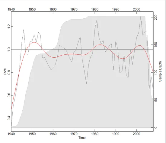
Tree core samples where the outermost part of the cores was intact, and the centre were unidentifiable, were included in the study since it was still possible to date them. However, the samples where the year rings were hard to define, and the stems were too damaged to provide reliable data, were excluded from the study. The final sample depth is illustrated as the grey zone in figure 3.
Figure 3: Sample depth of all sites combined, illustrated with the grey area in the graph. The red line
in the graph is the fitted spline function. The black line represents the average ring width index (RWI).
After the coordinates were set, the data was imported for dating to the software Cdendro. When all the samples were dated, the quality of the dating was controlled using COFECHA, a quality-control computer program developed by Richard Holmes (Speer, 2010). COFECHA is a free software that is used to find irregulari-ties in the chronologies. The program fits individual trees, takes residuals and aver-ages them to build a master chronology. The core to be analysed is removed from the master chronology, cut into 40-year segments with 20 years of overlap, and sta-tistically correlated against the master chronology. The chronologies signalling a low correlation with the master chronology were doublechecked in Coorecorder.
2.3 Data analysis
To continue, the ring width data was imported to R studio. R studio is a free software used by statisticians and researchers all over the world to analyse and process data (RStudio Team, 2016).
2.3.1 Basal Area Increment
Analysing growth trends using ring width data can be done by calculating the Basal Area Increment (BAI). BAI calculations are based on the assumption that the ring circumference can be estimated by a circle (Biondi & Qeadan, 2008). This method is preferred by Martin-Benito et al (2010), arguing that BAI is less dependent on age than other ways of analysing tree rings are. Therefore, the need for detrending can be avoided. By subtracting the area of a cross-section in year t-1 from that in year t, annual growth increments can be calculated (Speer, 2010). Moreover, BAI was a suitable method since it was the year-to-year difference in each plot that was being investigated, not the difference in growth-trends between the sites. The BAI curve for the control plot was visually interpreted and extreme years were selected for further analysis. I created one list with years where the BAI was high and one where it was low. The years where the treatments correlated with the control plots were given a “0”, and the years where the growth differed from the control was given a “1” (See table 3 and 4).
2.3.2 DplR package
Detrending is carried out to assure that long term effects depending on stand dy-namics and tree age are removed (Bunn, 2010). It was needed to detrend the ring width data to execute the weather and growth correlation analysis provided by the treeclim library package. The DplR package is developed to offer the possibility to analyse tree core data using R studio. The package made it possible to import the file format which contained the ring width chronologies. The main idea of the pack-age is that it should be used to carry out analysis concerning chronology building and cross dating (Bunn, 2008).
2.3.3 Treeclim package
To investigate the correlation between weather and growth, the R package “treeclim” was used. The package is based upon a MATLAB function created to summarize the seasonal climate signal in a tree ring series (Meko et al, 2011). The package uses a simple Pearson correlation coefficient. Treeclim is mainly used for dendrochronological applications; however, it has proved useful for other annually resolved natural archives as well (Zang and Biondi, 2015). To execute the analysis “seascorr” it is necessary to have dated tree ring chronologies and at least two vari-ables of climate data representing all 12 months of the year. Monthly precipitation was set as the primary variable and monthly mean temperature as the secondary. In the results, the average six months correlations are presented in the result. The ring width chronologies are divided into years before first thinning and after first thin-ning.
2.3.4 Weather data
Weather data specific for each site was collected from SMHI, who used the global model JRA 55 (Harada et al., 2016) to create a comprehensive and useful data set. The model is named after the Japanese 55-year Reanalysis (JRA-55) and is gridded with high 15 spatial resolution starting in 1958. The model includes observations from for example weather stations, satellites and radiosondes. Each site has been matched with the weather data from the closest weather stations to provide the most accurate simulation of the weather conditions as possible. The most important thing for this study was that data for each month could be provided. The weather variables monthly precipitation and mean temperature was used for the analysis conducted in this study.
Figure 4- 8: Precipitation index for each site, starting from 1958 and continuing until the year when
3.1 Basal area increment
The BAI for each treatment was visually interpreted to identify growth differences between the treatments (figure 9 – 13). Higher thinning grades gave a stronger re-sponse in BAI. The larger removal of trees in treatment C resulted in an increase in growth for the remaining trees some years after thinning (red lines), whereas the smaller and more frequent thinnings in treatment A and E resulted in a more even increase in BAI but no peak as high as in treatment C (orange lines). Thus, it can be assumed that different treatments result in different ring width growth, at least the years after a thinning is carried out.
Figure 9 - 13: BAI (cm2/year) for each treatment on each site. The control treatment is the green line,
the red line treatment C and the orange treatment A/E. The vertical, dotted lines mark the thinning years. The red line marks thinning years for treatment C, and the orange lines mark the tinning years for treatment A/E. The purple dotted lines mark years when both treatment C and A/E were thinned.
3.2
Comparison of years with high BAI in control plot
To further investigate whether different treatments affected ring width growth dif-ferently, the years in the control plots with distinct increase or decrease in BAI were chosen to check how well the treated plots correlated with the control plots (Figure 14 – 17).
Figure 14- 17: Control treatment for each site with red dotted lines marking the extremely low BAI
For years with decrease in BAI, some interesting differences could be identified. The proportion of years when thinned plots responded differently than the control was 5/24 for the C-treatment and 8/24 for the A/E-treatment (Figure 9). However, the analysis also indicates that, especially for the A/E treatment, it is unlikely that thinned treatments always respond in a similar way as the control when its growth decreased.
Table 3: Extreme years in BAI for the control plots when the growth was unusually low and how they
correlated with the treatments. If they reacted the same, the years received the number “0”. If they reacted differently, the years received the number “1”.
Year Site 901 Site 920 Site 941 Site 943 Treat. C Treat. E Treat. C Treat. E Treat. C Treat. A Treat. C Treat. A 1968 - - - - 1 0 - - 1969 - - 1 0 - - - - 1975 - - - - 0 0 - - 1976 - - 0 0 - - 0 1 1978 - - - - 0 1 - - 1979 - - - 1 1 1983 - - - - 0 1 0 0 1985 0 1 0 0 - - - - 1986 - - - 0 0 1989 0 0 - - 0 0 0 0 1992 0 1 0 0 - - - - 1993 - - - - 1 0 0 1 1995 - - - 0 0 1996 1 1 0 0 - - - - 1998 - - 0 0 0 0 - - No. of 1 1 3 1 0 2 2 1 3
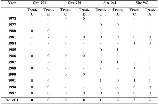
The years when BAI was high did not provide enough years with different responses to be interesting for further analysis. It was clear that if the control plot reacted with increased growth the treatments would do so as well (table 4).
Table 4: Extreme years in BAI for the control plots when the growth was unusually high and how they
correlated with the treatments. If they reacted the same, the years received the number “0”. If they reacted differently, the years received the number “1”.
Year Site 901 Site 920 Site 941 Site 943 Treat. C Treat. E Treat. C Treat. E Treat. C Treat. A Treat. C Treat. A 1973 - - 0 0 - - - - 1977 - - - - 0 0 - - 1980 0 0 - - - - 1981 - - 0 0 0 0 0 0 1984 - - - 1 0 1985 - - - - 0 1 - - 1986 0 0 0 0 - - - - 1987 - - - - 0 1 - - 1988 0 0 - - - - 1 1 1990 - - 0 0 - - - - 1991 0 0 - - 1 0 1 1 1994 0 0 - - - - 0 0 1997 0 0 0 0 0 0 0 0 No. of 1 0 0 0 0 1 2 3 2
3.3 Growth and weather analysis
The RWI for each treatment on each site was plotted against the summer precipita-tion, for the purpose of interpreting and trying to find any correlations between growth and precipitation (appendix 1, figure 25 - 29). However, no similar pattern between treatments on different sites and how they reacted to different precipitation levels could be observed.
Figure 15 – 19: Ring width indices and summer precipitation indices for each treatment on each site.
The control treatment is the green line, the red line treatment C and the orange treatment A/E. The blue, dotted line is the summer precipitation index.
3.2.1 Treeclim analysis
The precipitation and growth correlations were further analysed with the R package treeclim. In the treeclim correlation analysis, a positive correlation between precip-itation and growth could be found for September - December for treatment A/E be-fore thinning (figure 20). No correlation could be found for treatment C bebe-fore and after thinning (figure 24 and 26), nor for treatment E/A after thinning (figure 22).
Figure 20 and 21: Treatment A/E before thinning. All years before thinning are aggregated and their
correlation with the weather conditions is tested using a simple Pearson correlation. The graphs show the correlations between precipitation and growth over time as primary variable and mean temperature and growth over time as the secondary variable. The diagram to the left shows the correlations for the same period but in the in the control plots.
Figure 22 and 23: Treatment A/E after thinning. All years after thinning are aggregated and their
correlation with the weather conditions is tested using a simple Pearson correlation. The graphs show the correlations between precipitation and growth over time as primary variable and mean temperature and growth over time as the secondary variable. The diagram to the left shows the correlations for the same period but in the in the control plots.
Figure 24 and 25: Treatment C before thinning. All years before thinning are aggregated and their
correlation with the weather conditions is tested using a simple Pearson correlation. The graphs show the correlations between precipitation and growth over time as primary variable and mean temperature and growth over time as the secondary variable. The diagram to the left shows the correlations for the same period but in the in the control plots.
Figure 26 and 27: Treatment C after thinning. All years after thinning are aggregated and their
corre-lation with the weather conditions is tested using a simple Pearson correcorre-lation. The graphs show the correlations between precipitation and growth over time as primary variable and mean temperature and growth over time as the secondary variable. The diagram to the left shows the correlations for the same period but in the in the control plots.
The weather – growth treeclim analysis for the control plots showed no correlation with precipitation. However, there was a negative correlation between mean autumn to early winter temperature and growth in the control plots and the thinning treat-ment A/E (figure 21). There was no significant correlation between the two param-eters and growth in the period after thinning in treatment A/E (figure 23). No sig-nificance was found before or after thinning in the control plots when their weather correlation with growth was analysed for the same periods as treatment C (Figure 25 and 27).
4.1 Basal Area Increment
The results of this study confirm that thinning has an impact on BAI, and it is pos-sible that this correlation is due to the lowered competition for resources entailing the reduction of trees at the plots. The BAI curves showed a pattern well in-line with the observations made by Nilsson et al (2010). A heavy thinning like treatment C changed the growth pattern while “normal” thinnings did not result in significantly different ring-width pattern compared to the control pattern. It confirms the results by Martin-Benito et al (2010), who also found trees in heavier-thinned stands to grow faster. Martin-Benito et al (2010) related some of the result to the fact that it was the trees in the control plot that grew slower when no thinning was conducted than trees growing faster in heavier-thinned stands. This reflexion should be taken into consideration when interpreting the result of this study as well.
The hypothesis concerning tree growth and weather variations predicts that conducting thinnings makes the trees less vulnerable to weather variations. The analysis of extreme years indicated that the treatments reacted approximately the same as the control plots when the growth was high. However, during some of the years when growth decreased in control plots, growth of thinned plots did not re-spond in a similar way. Thus, the results of this study suggest that thinnings might increase the resistance to growth reducing conditions. Magruder et al (2013) came to a similar conclusion, since they found that thinning from below could reduce the response to climatic stresses. They did, however, conduct their study in Red pine stands. The different properties of Norway spruce and Red pine should be consid-ered when comparing the study by Magruder et al (2013) with the results in this report. Nevertheless, Norway spruce is a drought sensitive species (Bergh, 2005), and should therefore react similarly to the red pine, if not show a stronger correla-tion.
The reason for using BAI and not RWI was to prevent the calculations from buffering away some of the thinning response, a method recommended by Speer (2010) and used by, among others, Martin-Benito et al (2010). However, the pattern did not differ greatly from the ring width index, thus the latter was used to visualize summer precipitation and growth correlations.
Identifying extreme years to analyse is an approach used by Suvanto et al (2017) as well. However, they used an R package to identify the years. An advantage with this method is that human errors are easier to avoid, the sample of extreme years should be more accurate and objective. However, it is not certain that the method would have worked with the chronologies in this study, as they were much shorter. It is possible that no pointer years at all would have been found.
4.2 Growth and weather analysis
The results from this study cannot confirm that thinnings make trees less vulnerable to weather variations. Nor can they confirm that positive thinning response is af-fected by weather conditions in combination with the thinning treatment. The result suggests that the correlation depends more on individual variation than a general pattern. Other studies have found early summer precipitation to be of significant importance for individual tree growth (Ols et al., 2017., Martin-Benito et al., 2010). Martin-Benito et al (2010) suggested that conducting thinnings works as a buffer to rough weather conditions, though no such statement can be confirmed by this study.
Tree growth response to weather conditions might change with age (Speer, 2010). Several studies suggest that a tree’s response to weather variations depends on tree age. Nevertheless, the results are suggesting different things. Zang et al (2012) found that for Norway spruce stands, larger trees were more sensitive to cli-mate variables such as temperature and precipitation. Ding et al (2017) also found that young trees are more resistant to drought. Hence, doing an analysis comparing weather-growth correlations before and after thinnings might give us an answer to how trees at different ages respond to weather rather than how the treatments affect weather response. However, all trees in this study are still relatively young and age might not have an impact on the weather response yet. In a study conducted by Zhang et al (2018), they found that in wetter areas younger trees were more sensitive to weather variations than older trees. In drier sites, a stronger sensitivity to precip-itation was observed in August, September and May. On the other hand, older trees (between 120 – 140 years) showed correlation with summer temperature factors. In addition, Suvanto et al (2017) suggests that within-species differences should be considered. It might be the case that the result, to some extent, can be related to provenances and other within-species differences. The difference that can occur within a species should be investigated since it could lead to more informed choices when planting. Investigating the effect of provenances on drought resistance has already been done to some extent and could possibly be an interesting way to move forward with this research.
4.3 Site selection
For this report, three different stand densities and one control treatment were cho-sen. The primary choice would have been only three treatments represented on each site. However, due to storm damage, this was not possible and where treatment A
was absent it was replaced with treatment E. To avoid pseudoreplication as de-scribed by Hurlbert (1984), four different sites were chosen. Nevertheless, it is im-portant to note that the number of cores from some plots were very small. Hence, they might not be representative for the treatment, a fact which should be taken into consideration when interpreting the results.
4.4 Sample quality and sample depth
Only one sample was obtained from each tree. Since trees often grow irregularly, there is a risk that samples are not representative of the growth of the entire tree. This is also pointed out as problematic by Biondi (1999). Furthermore, he mentions asymmetric pith location as a source of uncertain measurements. Čermák et al (2017) conducted a study similar to this one and they only extracted one core as well, with the motivation that variability between trees within a plot is higher than the variability within the tree around the stem. Radial shrinking of the cores as they dry is, according to Biondi (1999), minimal although it will to some extent reduce the estimated growth rate.
The coordinates were to be put out in a perpendicular angle to the year ring, however it could sometimes be difficult to do so, since some cores had rings with strong curvatures due to wrongly extracted samples in the forest or damage to the tree. For example, a leaning tree could have developed extra wood in one direc-tion to strengthen itself and keep from falling, meaning wouldn’t give a representa-tive image of the growth-weather relationship. The optimal scenario would have been to have disks of each tree and calculate a mean value of the distances between the rings. However, this is easier to do for small rings, and working with data already collected more than ten years ago made it impossible.
It is recommended by Speer (2010) to have a sample depth of at least 30 living trees and two cores from each tree in order to have a robust sample depth. If the sample depth goes under 10 or 20 trees, the risk that growth variations of indi-vidual trees overwhelm the common growth signal. This criteria for a robust sample depth could not be fulfilled in this study, due to different factors that could not be helped. It is a major aspect to consider when interpreting and analysing the results. Containing data from one of the largest thinning experiments of its kind is definitely one of the strengths of this study, however it becomes a weakness in terms of repli-cability. Ideally, the study should be repeated, starting with a data collection aiming specifically to provide data for this type of study. Finding another thinning experi-ment of the same magnitude and the same treatexperi-ments present can prove to be a dif-ficult task.
4.5 Scientific importance of the project
The warm and dry summer in 2018 made more people aware of the fact that human activities will need to change in the future in accordance with changing climate con-ditions. Forest resources are for many the key to sustainable development and
cli-mate change adaptation. Earlier thinning research has often focused on growth pro-duction (Nilsson et al, 2010), whereas studies like this put it in relation to climate factors, a necessary approach if we are to grow healthy forests that can contribute to climate change adaptation. In fact, it is possible that forests with high production are the most sensitive to weather variations and thus not sustainable. Another im-portant aspect is that forests today are subject to multiple goals (Beland-Lindahl et al, 2015). They are expected to hold high biodiversity and recreational values, ab-sorb CO2 and provide timber. For one and the same forest to perform equally good on all these points is a challenge yet without a solution. Klapwijk et al (2018) do in their article “Capturing complexity: Forests, decision-making and climate change mitigation action” trace the inability to adapt forest management to climate change to market uncertainties, lack of incentives to change and a disagreement of “accepta-ble forest use”. We need to move forward, alas the direction remains unclear.
Thinning is no guarantee for increased production volume; on the con-trary, unthinned stands can hold bigger volumes although the mean diameter growth will be lower (Nilsson et al, 2010). The main argument for thinning does not lie in its capability to increase stand volume. Rather, the advantages are connected to in-creased quality of individual trees, nature management operations and reduced com-petition between the trees. Interspecific comcom-petition can weaken a forest stand and make it susceptible to pests and insects, thus it is possible that thinnings can increase the resilience on a stand level (Martin-Benito, 2010). There is currently no consen-sus in this area and more research is needed.
Sweden is a small country with a surprisingly large influence on forestry and forest research. It is also one of the richest and most developed countries in the world, hence we have a responsibility to lead and to be a pioneer in the conversion to a climate neutral society. Conducting meaningful research that can contribute and be applied in other countries as well is one way to take on this responsibility. Further thinning studies should therefore hold this as an important aspect when forming re-search projects and questions to be answered.
4.6 Further research and recommendations
Pukkala et al (2016) found in their study about wind damage that even-aged stands with repeated low stem removals, much like the thinning treatments A and E in this report, are highly susceptible to storm damage. Furthermore, Nilsson et al (2010) found that the traditional thinning program with three thinnings from below did not increase the stand volume. These results in combination with the result of this report, indicating no advantage for individual stem growth when following treatment, A or E, question the traditional way of conducting forest management operations. Nev-ertheless, the results from Martin-Benito (2010), Magruder (2013) and Giuggiola et al (2013) must not be forgotten. There are implications that thinning increases a stand’s resilience to climatic variations, which should be considering when conduct-ing research to formulate new thinnconduct-ing guidelines. Future, similar studies should take care to include a larger sample size and perhaps even other tree species, in order to gain a broader understanding of how thinning response is connected to weather variations.
Thinning operations and how they are carried out might play an important role in climate change adaptation. This study confirms that different thinning programs af-fect ring width growth in Norway spruce monocultures differently, heavier thin-nings leads to an immediate increase in ring width growth for the remaining trees. The same trend can be observed in stands with lower thinning rates however not as evident.
The weather-growth relationship was harder to distinguish. There were indications that the treated plots had higher resilience to growth reducing events. When the Basal Area Increment was low in the control plot, it sometimes increased for the treated plots. However, the difference was not significant. When analysing the weather-growth relationship using the R package treeclim, there were no clear indications that the plots reacted different before or after thinning.
Some of the results may be explained by the small sample depth. Another study with a larger sample could contribute to the knowledge about how thinning operations can be conducted in the future for resilient and climate-change-adapted forests.
Agestam, E. (2015). Gallring. Skogsskötselserien, kapitel 7. Second edition. Link to source: www.skogsstyrelsen.se/skogsskotselserien. 2019-04-15.
Beland-Lindahl, K., Sténs, A., Sandström, C., Johansson, J., Lidskog, R., Ranius, T. and Roberge, J. (2015). The Swedish forestry model: More of everything?. Forest Policy and Economics, 77, pp.44-55.
Bergh, J., Linder, S. and Bergström, J. (2005). Potential production of Norway spruce in Sweden. Forest Ecology and Management, 204(1), pp.1-10.
Biondi, F. (1999). Comparing Tree-Ring Chronologies and Repeated Timber Inven-tories as Forest Monitoring Tools. Ecological Applications, 9(1), p.216.
Biondi, F. and Qeadan, F. (2008). A Theory-Driven Approach to Tree-Ring Stand-ardization: Defining the Biological Trend from Expected Basal Area Increment. Tree-Ring Research, 64(2), pp.81-96.
Bréda, N., Granier, A., Aussenac, G., 1995. Effects of thinning on soil and tree water relations, transpiration and growth in an oak forest (Quercus petraea (Matt.) Liebl.). Tree Physiol. 15, 295–306.
Bunn, A. G. (2008). A dendrochronology program library in R (dplR). Dendro-chronologia, 26(2), 115–124. https://doi.org/10.1016/j.dendro.2008.01.002. Bunn, A. (2010). Statistical and visual crossdating in R using the dplR library. Den-drochronologia, 28(4), pp.251-258.
Čermák, P., Rybníček, M., Žid, T., Andreassen, K., Børja, I. and Kolář, T. (2017). Impact of climate change on growth dynamics of Norway spruce in south-eastern Norway. Silva Fennica, 51(2).
Ding, H., Pretzsch, H., Schütze, G., & Rötzer, T. (2017). Size-dependence of tree growth response to drought for Norway spruce and European beech individuals in monospecific and mixed-species stands. Plant Biology, 19(5), 709–719. https://doi.org/10.1111/plb.12596
Gauthier, S., Bernier, P., Kuuluvainen, T., Shvidenko, A. and Schepaschenko, D. (2015). Boreal forest health and global change. Science, 349(6250), pp.819-822. Giuggiola, A., Bugmann, H., Zingg, A., Dobbertin, M. and Rigling, A. (2013). Re-duction of stand density increases drought resistance in xeric Scots pine forests. Forest Ecology and Management, 310, pp.827-835.
Guillemot, J., Klein, E., Davi, H. and Courbet, F. (2015). The effects of thinning intensity and tree size on the growth response to annual climate in Cedrus atlantica: a linear mixed modeling approach. Annals of Forest Science, 72(5), pp.651-663. Götmark, F., Fridman, J., Kempe, G. and Norden, B. (2005). Broadleaved tree spe-cies in conifer-dominated forestry: Regeneration and limitation of saplings in south-ern Sweden. Forest Ecology and Management, 214(1-3), pp.142-157.
IPCC. (2014). Climate Change 2014: Synthesis Report. Contribution of Working Groups I, II and III to the Fifth Assessment Report of the Intergovernmental Panel on Climate Change [Core Writing Team, R.K. Pachauri and L.A. Meyer (eds.)]. IPCC, Geneva, Switzerland, 151 pp.
Harada, Y., H. Kamahori, C. Kobayashi, H. Endo, S. Kobayashi, Y. Ota, H. Onoda, K. Onogi, K. Miyaoka, and K. Takahashi. (2016). The JRA-55 Reanalysis: Repre-sentation of atmospheric circulation and climate variability. J. Meteor. Soc. Japan, 94, 269-302.
Heiskanen, J. and Mäkitalo, K. (2002). Soil water-retention characteristics of Scots pine and Norway spruce forest sites in Finnish Lapland. Forest Ecology and Man-agement, 162(2-3), pp.137-152.
Hurlbert, S. (1984). Pseudoreplication and the Design of Ecological Field Experi-ments. Ecological Monographs, 54(2), pp.187-211.
Hänninen, H. and Tanino, K. (2011). Tree seasonality in a warming climate. Trends in Plant Science, 16(8), pp.412-416.
Hänninen, H. (2016). Boreal and temperate trees in a changing climate. Springer, Dordrecht.
Karlsson, K., (2003). Fältarbetsinstruktion för skogsfakultetens beståndsbehand-lingsförsök. Sveriges Lantbruksuniversitet.
Klapwijk, M., Boberg, J., Bergh, J., Bishop, K., Björkman, C., Ellison, D., Felton, A., Lidskog, R., Lundmark, T., Keskitalo, E., Sonesson, J., Nordin, A., Nordström, E., Stenlid, J. and Mårald, E. (2018). Capturing complexity: Forests, decision-mak-ing and climate change mitigation action. Global Environmental Change, 52, pp.238-247.
Lagergren, F., & Jönsson, A. M. (2017). Ecosystem model analysis of multi-use forestry in a changing climate. Ecosystem Services, 26, 209–224. https://doi.org/10.1016/j.ecoser.2017.06.007.
Larsson, L., (2003). CooRecorde & CDendro: Image Coordinate Recording and Da-ting Programs. Cybis Elektronik & Data AB, Saltsjöbaden, Sweden.
Lodin, I., Brukas, V., & Wallin, I. (2017). Spruce or not? Contextual and attitudinal drivers behind the choice of tree species in southern Sweden. Forest Policy and Eco-nomics, 83, 191–198. https://doi.org/10.1016/j.forpol.2016.11.010.
Magruder, M., Chhin, S., Palik, B. and Bradford, J. (2013). Thinning increases cli-matic resilience of red pine. Canadian Journal of Forest Research, 43(9), pp.878-889.
Martín-Benito, D., Del Río, M., Heinrich, I., Helle, G. and Cañellas, I. (2010). Re-sponse of climate-growth relationships and water use efficiency to thinning in a Pi-nus nigra afforestation. Forest Ecology and Management, 259(5), pp.967-975. Meko, D., Touchan, R. and Anchukaitis, K. (2011). Seascorr: A MATLAB program for identifying the seasonal climate signal in an annual tree-ring time series. Com-puters & Geosciences, 37(9), pp.1234-1241.
Nilsson, U.; Agestam, E.; Ekö, P-M.; Elfving, B.; Fahlvik, N.; Johansson, U.; Karls-son, K.; Lundmark, T.; Wallentin, C. (2010). Thinning of Scots pine and Norway spruce monocultures in Sweden—Effects of different thinning programmes on stand level gross and net stem volume production. Stud. Forest. Suec., 219, 1-46.
Nilsson, U., Fahlvik, N., Johansson, U., Lundström, A. and Rosvall, O. (2011). Sim-ulation of the Effect of Intensive Forest Management on Forest Production in Swe-den. Forests, 2(1), pp.373-393.
Nilsson, U., (2013). Skogens skötsel. Rapport från Future Forests 2009–2012, Swe-dish University of Agricultural Sciences, Umeå.
Ols, C., Trouet, V., Girardin, M. P., Hofgaard, A., Bergeron, Y., & Drobyshev, I. (2018). Post-1980 shifts in the sensitivity of boreal tree growth to North Atlantic Ocean dynamics and seasonal climate. Global and Planetary Change, 165, 1–12. https://doi.org/10.1016/j.gloplacha.2018.03.006.
Pukkala, T., Laiho, O. and Lähde, E. (2016). Continuous cover management reduces wind damage. Forest Ecology and Management, 372, pp.120-127.
RStudio Team (2016). RStudio: Integrated Development for R. RStudio, Inc., Bos-ton, MA URL: http://www.rstudio.com/.
Speer, J. (2010). Fundamentals of tree-ring research. Tucson, Ariz.: The University of Arizona Press.
Statistiska centralbyrån (SCB). Regionala indelningar. Link to source:
https://www.scb.se/hitta-statistik/regional-statistik-och-kartor/regionala-in-delningar/ 2019-05-15.
Suvanto, S., Henttonen, H. M., Nöjd, P., Helama, S., Repo, T., Timonen, M., & Mäkinen, H. (2017). Connecting potential frost damage events identified from me-teorological records to radial growth variation in Norway spruce and Scots pine. Trees, 31(6), 2023–2034. https://doi.org/10.1007/s00468-017-1590-y.
Suvanto, S., Nöjd, P., Henttonen, H. M., Beuker, E., & Mäkinen, H. (2016). Geo-graphical patterns in the radial growth response of Norway spruce provenances to climatic variation. Agricultural and Forest Meteorology, 222, 10–20. https://doi.org/10.1016/j.agrformet.2016.03.003.
Zang, C., & Biondi, F. (2015). treeclim: An R package for the numerical calibration of proxy-climate relationships. Ecography, 38(4), 431–436. https://doi.org/10.1111/ecog.01335.
Zang, C., Pretzsch, H., & Rothe, A. (2012). Size-dependent responses to summer drought in Scots pine, Norway spruce and common oak. Trees, 26(2), 557–569. https://doi.org/10.1007/s00468-011-0617-z.
Zhang, L., Jiang, Y., Zhao, S., Jiao, L., & Wen, Y. (2018). Relationships between Tree Age and Climate Sensitivity of Radial Growth in Different Drought Conditions of Qilian Mountains, Northwestern China. Forests, 9(3), 135. https://doi.org/10.3390/f9030135.