Comparing unsupervised
clustering algorithms to
locate uncommon user
behavior in public travel data
MAIN FIELD OF STUDY: Computer Science
A comparison between the K-Means and Gaussian
Mixture Model algorithms
Mail Address: Visiting address: Phone:
This thesis was conducted at Jönköping school of engineering in Jönköping within [see field of study on the previous page]. The authors themselves are responsible for opinions, conclusions and results.
Examiner: Maria Riveiro Supervisor: Beril Sirmacek
Scope: 15 hp (bachelor’s degree) Date: 2020-06-01
Abstract
Clustering machine learning algorithms have existed for a long time and there are a multitude of variations of them available to implement. Each of them has its
advantages and disadvantages, which makes it challenging to select one for a
particular problem and application. This study focuses on comparing two algorithms, the K-Means and Gaussian Mixture Model algorithms for outlier detection within public travel data from the travel planning mobile application MobiTime1[1]. The purpose of this study was to compare the two algorithms against each other, to identify differences between their outlier detection results. The comparisons were mainly done by comparing the differences in number of outliers located for each model, with respect to outlier threshold and number of clusters. The study found that the algorithms have large differences regarding their capabilities of detecting outliers. These differences heavily depend on the type of data that is used, but one major difference that was found was that K-Means was more restrictive then Gaussian Mixture Model when it comes to classifying data points as outliers. The result of this study could help people determining which algorithms to implement for their specific application and use case.
Keywords
Machine learning, clustering, K-Means, Gaussian Mixture Model, expectation-maximum, data analysis, public transport, silhouette analysis, outliers, outlier detection, data, algorithms, experiment.
Acknowledgments
We would like to thank Beril Sirmacek and Maria Riviero for their help and guidance during the process of writing this thesis. We would also like to thank Infospread Euro AB, as well as Vladimir Klicik and Gabriella Stenlund for being a helping hand throughout the whole study, and for providing the data and the hardware necessary to make this study possible.
1
Introduction ... 1
1.1 BACKGROUND ... 1
1.2 PARTNERING WITH INFOSPREAD EURO AB ... 1
1.3 PROBLEM DESCRIPTION... 2
1.3.1 Related work ... 2
1.4 AIM &RESEARCH OBJECTIVES ... 3
1.5 PURPOSE ... 3
1.6 SCOPE AND DELIMITATIONS ... 4
2
Theories ... 5
2.1 MACHINE LEARNING ... 5
2.2 CLUSTERING ... 5
2.3 OUTLIER DETECTION ... 5
2.4 K-MEANS ALGORITHM ... 6
2.5 GAUSSIAN MIXTURE MODEL ... 6
3
Method and implementation ... 7
3.1 EXPERIMENT DESIGN ... 7
3.2 EXPLORATION/PREPARATION OF DATA ... 8
3.2.1 Overview ... 8
3.2.2 The data - exploration and preparation ... 9
3.2.3 Region ... 10
3.2.4 Privacy concerns and GDPR ... 10
3.3 CONSTRUCTING BOTH THE MODELS ... 10
3.3.1 Using silhouette analysis to determine K (number of clusters) ... 10
3.3.2 Model construction ... 12
3.4 PICK APPROPRIATE THRESHOLDS FOR IDENTIFYING OUTLIERS ... 12
3.5 COMPARE RESULTS OF THE MODELS ... 13
3.5.1 Experiment 1 ... 14
3.5.2 Experiment 2 ... 17
3.6 ARTIFICIAL OUTLIER EXPERIMENT ... 19
4
Interpretation and analysis of the results ... 22
5
Discussions and conclusions ... 24
5.1 IMPLICATIONS ... 25 5.2 LIMITATIONS ... 25 5.3 RELIABILITY ISSUES ... 25 5.4 CONCLUSION ... 26 5.5 FUTURE WORK ... 27References ... 28
1
Introduction
Commuting is a day to day normal task for most people, and as such people usually follow basic patterns such as what station they enter or leave the bus, what type of ticket they purchase, and what bus they prefer to take. This study will show how to locate outliers in these patterns by modeling normal user behavior in the area of public transport, and then locating outliers within that model. The research will focus on implementing a mathematically distance-based algorithm (K-Means), and a statistical algorithm (Gaussian Mixture Model), and model the user behavior using both of them, to then compare the results that the two models produce.
1.1 Background
Data analysis, both exploratory and confirmatory, can be done in many ways these days. Clustering is a widely used algorithm for performing data analysis on datasets, and it can be done in many ways and can be utilized in many different areas. As given in [2] Even though there is an increasing interest in the use of clustering methods in
pattern recognition, image processing and information retrieval, clustering has a rich history in other disciplines such as biology, psychiatry, psychology, archaeology, geology, geography, and marketing.
A clear definition of what a cluster is, is given in [3] While analyzing data, a widely
used task is to find groups of dataset objects that share similar characteristics. In doing so, users gain insight into their data, understand it, and even reduce its high dimensionality nature. These conceptual groups are commonly referred to as clusters.
Clustering algorithms produce these clusters to organize and separate data into different groups, as described above, and this is the way clustering algorithms help perform data analysis, and in this case, outlier detection.
Anomaly detection, also known as outlier detection [4], is a way to find irregularities in data of any kind, as well as used with all types of data to find errors or problems with a dataset [5]. As mentioned before, the K-Means, and the GMM (Gaussian Mixture Model) algorithms are used in this study to perform the outlier detection. A crucial part of a GMM is the EM (expectation-maximum) algorithm which
according to [6] is a general method to improve the descent algorithm for finding the maximum likelihood estimation.
1.2 Partnering with Infospread Euro AB
This study was conducted in close cooperation with the software company Infospread2 Euro AB. They were interested in exploring the possibility of using AI and Machine Learning to analyze their users' travel data gathered from their app MobiTime [7], an app that delivers information commuters need in order to make decisions in the procedure of commuting. Infospread has, therefore, provided us with data and hardware required to carry out this study.
1.3 Problem description
There are a multitude of different algorithms to choose from when clustering data using machine learning. It can be hard to know which algorithm will work the best on your specific dataset, and which one will produce the best results. Very often there is not one algorithm that works best, but it is normally a trade-off, depending on the context and requirements of the task. This study will conduct several different experiments, to compare the results of two different unsupervised clustering algorithms. Different variables will be tweaked in between experiments such as algorithm parameters, data dimensionality and regularity, outlier detection thresholds and others, to provide a wide variety of comparisons to the reader.
Our collaborator will provide us with real-world, high quantity data, and analysis on the algorithms using specific subset(s) of the data will be performed. The study will, by using Infospread’s dataset, propose differences to consider in selecting one out of the two unsupervised machine learning algorithms, best optimized for finding patterns and anomalies in a dataset with comparable specific properties of dimensions and regularity.
1.3.1 Related work
Relevant related studies have been done on different clustering algorithms used in different contexts and areas. In Bacquet et al [8] they compare unsupervised clustering algorithms to monitor traffic data and evaluate two metrics from them, the detection rate, and false False negatives, in order to find the most effective clustering algorithm. In Laxhammar et al [9] research is done on the topic of anomaly detection on boat traffic, using data from sensors on vessels. They take on the challenge of anomaly visualization, where interactive visualizations are created so that humans can make sense of the dataset, and by analyzing the visualizations, can make their own
implications and conclusions of what is and is not an anomaly. Without the interactive visualization it would not be feasible for a human to scan through the raw sensor data to locate anomalies within the data.
In Van Craenendonck et al [10] a comparison of 5 different unsupervised clustering algorithms is made using internal validation methods. The specifics of the datasets that are used are not specified, but it is mentioned that they use a couple of different datasets coming from UCI3.
In Kuyuk et al [11] a comparison is made between K-Means and GMM by classifying seismic events in the vicinity of Istanbul. Since they are building classifiers, they mainly measure and compare performance and accuracy, which is not the case in this study.
1.4 Aim & Research Objectives
The aim of this study is to compare the two algorithms for finding outliers in public transport data, as well as analyzing the differences in the results that both the models produce.
This is done by constructing two models, using the same attributes from the dataset to model normal user behavior. This leads to differences in how the two algorithms have constructed the models, and the differences in how and what anomalies have been located between them will show.
The aim is answered with this research question:
• What differences can be found in outlier detection between the K-Means and GMM Clustering algorithms with respect to outlier threshold and number of outliers found?.
For each experiment both algorithms will process the same data attributes from Infospread’s dataset, to form two different cluster models. These models will then detect outliers within those models (using different thresholds for what counts as an outlier). Differences in the outlier detection within the two models will be compared and discussed.
In Abbas et al [12] they compared a multitude of different clustering algorithms, and some of the conclusions they made are:
• “The performance of K-Means and EM algorithms is better than hierarchical clustering algorithms”
• “The quality of EM and K-Means algorithms become very good when using huge datasets.”
These conclusions make it interesting to compare both of these algorithms, as they were “ranked” the same, and categorized as being similar in many ways. To isolate both algorithms and compare them could lead to unique findings.
1.5 Purpose
The purpose of this study is to compare the results of two different unsupervised algorithms that can detect outliers in travel data. Using a dataset which will then be input into two algorithms to further evaluate the difference of their outlier detection. This will further increase the knowledge on how travel data can be analyzed and how the two algorithms can improve the area of travel.
If differences are found during the experiments of the algorithms, it can guide developers in the right direction in which algorithm to use on their specific dataset.
1.6 Scope and delimitations
Public data in general is something most applications have the right to store, and as such the data can be tested and or studied for research of different kinds. Traffic data however is not included in the public data category so no data of any kind will be distributed in this study.
The focus of this study is not to research and discuss the inner workings of the algorithms, it will explain a little bit about the data used but nothing major about the algorithms. As for the located outliers, nothing will be concluded about what they are.
2
Theories
This chapter will summarize the different theoretical frameworks touched upon in this study. A conclusion that can be drawn is that this is a trending topic with a large number of research being conducted. This study, however, separates itself from the research area by conducting a unique result based comparative study, using a unique dataset never before used to conduct research
2.1 Machine learning
As stated in [13] The term machine learning refers to a set of topics dealing with the
creation and evaluation of algorithms that facilitate pattern recognition, classification, and prediction, based on models derived from existing data. Machine learning in recent
years has been developing more and more into different fields, going from analyzing biological data to metric data from search histories. Machine learning has also been going through an extensive development with mathematical complexity to further take on harder and harder tasks that humanity brings forth, most importantly the framework side of machine learning is ever expanding with new works. The frameworks can further test the validity of such machine learning programs [13].
2.2 Clustering
Clusters can be defined as “A set of entities which are alike, and entities from different clusters are not alike” but also “an aggregate of points in the test space such that the distance between any two points in the cluster is less that the distance between any point in the cluster and any point not in it”[14]. The focus on this study will be the latter of the two as the clustering algorithms will organize the data into different clusters, in this manner.
2.3 Outlier detection
According to statistical literature [15] An outlier is an observation which appears to
be inconsistent with the remainder of a set of data.
According to [16] Outlier detection has been used for centuries to detect and, where
appropriate, remove anomalous observations from data. Outliers arise due to mechanical faults, changes in system behaviour, fraudulent behaviour, human error, instrument error or simply through natural deviations in populations. Their detection can identify system faults and fraud before they escalate with potentially catastrophic consequences.
As mentioned in [15], outlier detection algorithms are useful in areas such as machine learning, data mining, pattern recognition, data cleansing, data warehousing and applications as: credit fraud detection, security systems, medical diagnostic, network intrusion detection and information retrieval.
2.4 K-Means Algorithm
The K-Means algorithm [17] is, as previously mentioned, a clustering machine learning algorithm. K-Means is essentially a partitioning method applied to analyze data as objects, where data points get partitioned into separate clusters based on Euclidean distances, such that data points within the same cluster stay as close as possible to each other, while being as far away as possible from data points from other clusters.
The K-Means algorithm can be separated into 5 different steps: 1. Set K - Decide number of clusters, K.
2. Initialization - Choose K starting points as centroids for each cluster. 3. Classification - inspect each data point in the dataset and assign it to the
cluster with the nearest centroid.
4. Centroid Calculation - After each data point from the dataset has been
assigned to a cluster, the centroids k need to be recalculated and repositioned. 5. Convergence Criteria - Repeat step 3 and 4 until no point changes cluster, or
the centroids do not move.
2.5 Gaussian Mixture Model
The GMM algorithm [18] is also a clustering machine learning algorithm. The difference between K-Means is that the GMM is a probabilistic model that instead of using Euclidean distances for classifying data points into clusters, it uses Gaussian distributions, where each data point is assigned a probability of the likelihood of it being part of a cluster in the model. This is done through a single-density estimation method with multiple gaussian probability functions, to generate the probability distribution within the model.
The GMM Algorithm can be separated into 4 steps: 1. Set K - Decide number of clusters, K.
2. Expectation - For each data point D, compute the membership probability of D in each cluster.
3. Maximization - Update mixture model probability weight.
4. Repeat step 2, 3 until stopping criteria is satisfied, I.E no further improvements can be made to the likelihood value.
3
Method and implementation
This study presents a comparison between the results of two different unsupervised clustering-based algorithms. What is compared are the differences in how the two algorithms manage to locate outliers in a dataset on traffic and commuting. The first algorithm is a mathematically distance based (K-Means), while the second one is a statistical algorithm (Gaussian Mixture) that relies on mathematical log probability to find outliers.
3.1 Experiment design
The experiments being conducted [19] must be systematic and sound. Therefore, planning and designing has carefully been done to validify the experiment process. The experiments need to produce quantifiable results for the comparison to be of any value, therefore a small range of quantifiable variables has been carefully chosen for comparing the algorithms in each experiment, as described in 3.5.
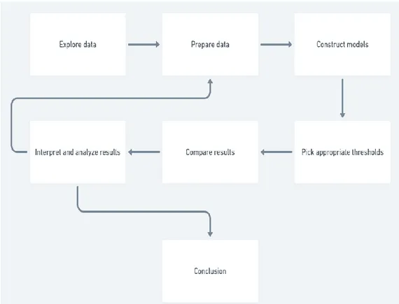
This is a quantitative comparative experimental study where comparisons of algorithms are made. To be able to make accurate comparisons of the two different algorithms, several steps were completed as listed below. The incremental loop can be seen in Figure 1.
• Dataset exploration. • Data preparation. • Model constructing.
• Pick appropriate thresholds.
• Compare, interpret, and analyze results. • Make the conclusion.
Figure 1 - The incremental loop of the experiment design and how the experiments are conducted.
As described in [2], A common strategy of performing outlier detection using clustering algorithms is to first create a model of the dataset as a whole, and in that model locate the outliers. Therefore, this method has been chosen to use in this research.
3.2 Exploration/Preparation of data
3.2.1 Overview
Before a decision is made on what data attributes from the dataset to use for an experiment, an exploration of what data is available within the dataset must be done. Data points that seem more valuable during exploration will be noted, so that they are more likely to be included during current, and future experiments.
Before the data is used to construct the clustering models, some preparation of the data might be necessary. The dataset will contain both numeric and categorical data, and since the sample space for categorical data does not have a natural origin, the distance between categorical data is not really meaningful, and could cause clusters to be formed that would ruin the experiment. To make the categorical data usable, a conversion would be made from categorical attributes to binary values.
The dataset being used in this study is rather large, and this is something that will be taken advantage of in this study, by partitioning it to smaller subsets more appropriate for the algorithms to model.
Each experiment is conducted in the exact same fashion, the only difference is the data that is used. For the first two experiments data is used from Inforspreads dataset, while the last experiment adds a couple of artificially generated data points, which in the real world would be considered outliers. This last experiment is conducted to investigate how well both the algorithms can locate actual outliers within the dataset. 3.2.2 The data - exploration and preparation
3.2.2.1 First experiment dataset
The first experiment of this study uses the travel search data that exists within the dataset. The attributes within the travel search data describe travel searches that users of Infospread’s app have executed. An example of this is when a user wants to search for a bus trip between two separate stations. How this data looks is shown in Table 1 below.
Table 1 - Travel search dataset attributes
How the first experiment uses the data is:
1. Count the amount of times users have searched for a journey from a specific station
2. Count the amount of times users have searched for a journey to a specific station
3. Put that data together in its own table, to prepare it to be clustered. After these steps, we end up with a table that looks like Table 2 below.
Table 2 - Station travel count dataset 3.2.2.2 Second experiment dataset
The second experiment of this study also uses travel search data, but in a very different way. This experiment uses search data from when a user has searched for a journey from a location that is not a station. The table contains other vital information such as when the search happened, what user performed the search, and in what region the search happened. How this data looks is shown in Table 3 below.
How the second experiment uses the data is:
1. Include the distance to the nearest station from Table 3.
2. Convert the Unix timestamp from Table 3, to minutes passed on that day for each entry in the dataset.
3. Put that data together in its own table, to prepare it to be clustered. After these steps, we end up with a table that looks like Table 4 below.
Table 4 - Travel search station data. Contains time which is when the search is made and the distance to the nearest stop station.
Two 2-dimensional datasets are now ready and prepared, which means that it is possible to move on to the next step of using both of the clustering algorithms to construct both of the models.
3.2.3 Region
The specific dataset is retrieved from the region Jönköping in Sweden and only contains data from that region.
Table 5 - Number of bus stations in the Jönköping (JLT) region.
3.2.4 Privacy concerns and GDPR
The data used has been collected implicitly, this is simply the user’s history while using and searching within the application. The study and its data will be coherent to GDPR law by using data not traceable to persons, history of travel and commuter pattern are synonymous with device trajectory but never to any personal profiling data.
3.3 Constructing both the models
3.3.1 Using silhouette analysis to determine K (number of clusters)
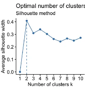
A common problem when implementing clustering algorithms is to determine how many clusters should be created for each model. A solution to that is to perform a silhouette analysis using scikit-learn4[20] . A silhouette analysis will study separation distances between the resulting clusters, to try and display a measure of how close each point in one cluster is to points in the neighboring clusters. In Figure 2 an example is shown of how a silhouette analysis has tested a couple of different numbers of clusters, to find the optimal one.
A silhouette analysis is performed before every experiment, to locate the optimal number of clusters for the specific data attributes used. This does not limit the experiment to only the cluster amount that the silhouette analysis recommends, but rather serves as a base for where to start the experiment.
It is not feasible to blindly follow a recommendation from the silhouette analysis, as it knows nothing about the context of the data. Therefore, the recommendation from the silhouette analysis must be analyzed and compared with the context of the data, to verify that the recommendation makes sense.
A silhouette analysis is done to discover how many clusters to use in each respective experiment.
For the first experiment, the analysis showed that the optimal cluster amount to use for the attributes from Table 2 is two clusters. Two clusters make sense in this case, since the number of searches from/to different stations can be categorized into two different groups: stations with a low search rate, and stations with a high search rate. For the second experiment, the silhouette analysis delivers a very different result compared to the first experiment. This time the silhouette analysis showed that the optimal cluster amount for the data attributes from Table 4 is six clusters. This is not quite as easy to justify as the first experiment, but when you inspect the resulting separation of the data, it becomes clearer that a higher number of clusters is needed, since the data is very diverse. This is mainly true because the data used, as seen in
Table 4 has the minutes passed on current day included as one of the parameters,
and thus the data spreads out during each day, which leads to a diverse separation of many data points
Figure 2 - Silhouette example for measuring clusters and determining appropriate number of clusters. In the graph, two clusters get the highest silhouette width, and is therefore the
3.3.2 Model construction
Before each experiment, both the clustering models are constructed with the same number of clusters and the same data attributes. The scikit5[20] library is used for implementing both the clustering algorithms, which is available in Python.
For the first experiment both models initially get constructed with a parameter of 2 clusters, and they get fitted with the exact same data attributes, as shown in Table 2. For the second experiment both models also initially get constructed with a parameter of 6 clusters, and they also get fitted with the exact same data attributes, as shown in
Table 4.
3.4 Pick appropriate thresholds for identifying outliers
To make sure the comparison is of any relevance, appropriate thresholds must be calculated for what gets labeled as an anomaly and what is not.
Since K-Means and GMM use different units to measure how much a data point belongs to a certain cluster, a unified way to determine appropriate thresholds for both the algorithms needs to exist.
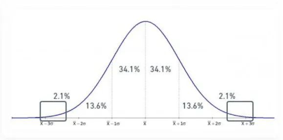
As mentioned in [21], a very common and unified way of determining the thresholds is to use the mean value of the data in the model plus two or three standard deviations. This experiment initially uses three standard deviations as shown in Figure 3. This way data is partitioned out to a small subset of the models outside the outlier detection thresholds. From there we can then move both the thresholds in both positive and negative directions with percent-based steps, to maintain the appropriate scale of the thresholds.
Figure 3 - Standard deviation range of outlier detection. The red squares show the areas where outlier detection thresholds are set and is therefore also where the outliers are located
within the model.
5 Scikit is a python library that can be used for predictive data analysis, read more about it here
To consider every data point located outside of 3 standard deviations as an outlier is of course an assumption that is made, this does not mean that every data point that meets this criterion, in reality is in fact an outlier. It is fully possible that it can just be an uncommon data point. This assumption makes it possible to classify data points as outliers or not based on unified thresholds, which in return makes this study’s finds quantifiable and directly comparable, by discovering suitable metrics to compare. Since both algorithms use different units for determining cluster belongings, the threshold will look different for each algorithm. In upcoming figures in this study, you will be able to see different threshold numbers between K-Means and GMM comparisons, where the K-Means threshold is usually a higher number. This is because the mean Euclidean distances plus three standard deviations are usually a lot higher than the mean log-probabilities plus three standard deviations.
3.5 Compare results of the models
After the cluster models have been constructed, they are compared against each other. For both the models, a parameter is set to determine what is considered an outlier. For the K-Means cluster this parameter is the Euclidean distance between the cluster point and the nearest centroid6, as shown in Figure 4. For the GMM, the parameter is a
weighted log probability of each point in the model, of how likely the point is to belong to a cluster in the model as illustrated in Figure 5.
Figure 4 - Euclidean distance example between P1 and P2. The parameter for determining what is considered an outlier or not in the K-Means Model, in relation to a given threshold.
Figure 5 - GMM weighted log probabilities example on a 3-cluster model. These probabilities are the parameters for determining what is considered an outlier or not in the GMM
When comparing the results from both models, we focus on the number of outliers both the algorithms find, per threshold.
3.5.1 Experiment 1
This experiment uses the data from Table 2, and the silhouette analysis recommended starting with 2 number of clusters, then we perform the same experiment but with 3 clusters instead.
3.5.1.1 - 2 Clusters
When using two clusters (the silhouette analysis calculated this to be the optimal number), both of the algorithms start off finding a slightly different amount of outliers, but as the threshold decreases, they start to approach the same amount as displayed in Figure 6 and Figure 7 below.
K-Means threshold is the mean centroid distance of each point in the dataset plus 3 standard deviations, this means that the mean distance plus three standard deviations start at slightly less than 8000 and increases per iteration of the experiment as shown in Figure 6.
GMM threshold is the mean log-probability value of each point in the dataset plus 3 standard deviations, this means that the mean log-probability value plus 3 standard deviations, starts at slightly above 20 and increases per iteration of the experiments as shown in Figure 7.
On the Y axis of each histogram figure below, the number of outliers shows the absolute number of outliers located, which means that for K-Means when the threshold was slightly less than 8000 it found 18 outliers which is 1.58% of the dataset. For GMM when the threshold was slightly above 20 it found 15 outliers which is 1.32% of the dataset as illustrated in Figure 6 and Figure 7.
The histogram figures below display outliers found from the dataset, where each datapoint is a search a user has performed within the application.
Figure 6 - Experiment 1. K-Means outliers 2 clusters, X-axis is the calculated threshold which in this case is the mean centroid distances of each point in the dataset plus 3 standard deviations and then an increase per iteration of the experiment, Y-axis is the number of
outliers located per threshold.
Figure 7 – Experiment 1. GMM outliers 2 clusters, X-axis is the calculated threshold as a log-probability of a point belonging to a certain cluster and then an increase per iteration of the
3.5.1.2 – 3 clusters
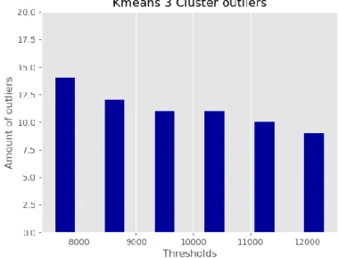
When using three clusters ( the silhouette analysis did not calculate this to be the optimal number), the algorithms are fairly different than when using two clusters. On the lowest threshold, the GMM finds more outliers than K-Means, but on the higher thresholds, it finds less outliers than K-Means, as displayed in Figure 8 and Figure 9 below.
Figure 8 - Experiment 1. K-Means outliers 3 clusters, X-axis is the calculated threshold which in this case is the mean centroid distances of each point in the dataset plus 3 standard deviations and then an increase per iteration of the experiment, Y-axis is the number of
outliers located per threshold.
Figure 9 - Experiment 1. Gaussian Mixture outliers 3 clusters, X-axis is the calculated threshold as a log-probability of a point belonging to a certain cluster and then an increase per iteration of the experiment, Y-axis is the number of outliers located per threshold.
3.5.2 Experiment 2
This experiment uses the data from Table 4, and the silhouette analysis recommended starting with 6 number of clusters, then we perform the same experiment but with 7 clusters instead. The difference between the first experiment is that the data that is used for this experiment contains a temporal component.
3.5.2.1 - 6 clusters
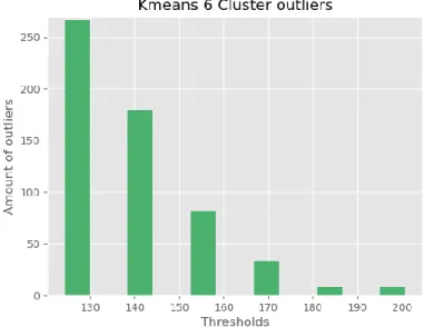
When using six clusters, as displayed in Figure 10 and Figure 11 below, both
algorithms start off being quite different on the higher thresholds. K-Means finds less than 10 outliers which is 0.05% of the dataset, while GMM finds over 200 outliers which is 1% of the dataset. As the threshold decreases, K-Means starts finding more and more outliers but still does not surpass the amount that GMM finds even at the lowest threshold.
Figure 10 - Experiment 2. K-Means outliers 6 clusters, X-axis is the calculated threshold which in this case is the mean centroid distances of each point in the dataset plus 3 standard
deviations and then an increase per iteration of the experiment, Y-axis is the number of outliers located per threshold.
Figure 11 - Experiment 2. GMM outliers 6 clusters, X-axis is the calculated threshold as a log-probability of a point belonging to a certain cluster and then an increase per iteration of the
experiment, Y-axis is the number of outliers located per threshold. 3.5.2.2 - 8 clusters
When using eight clusters, as displayed in Figure 12 and Figure 13 below, Both the algorithms act almost the same as when using 6 clusters, only the K-Means outlier detection amplitude is lowered, for each threshold.
Figure 12 - Experiment 2. K-Means outliers 8 clusters X-axis is the calculated threshold which in this case is the mean centroid distances of each point in the dataset plus 3 standard deviations and then an increase per iteration of the experiment, Y-axis is the number of
Figure 13 - Experiment 2. GMM outliers 8 clusters, X-axis is the calculated threshold as a log-probability of a point belonging to a certain cluster and then an increase per iteration of the
experiment, Y-axis is the number of outliers located per threshold.
3.6 Artificial outlier experiment
On the first dataset as shown in Table 1, two different types of experiments are carried out with the algorithms. The first one only uses Infospread’s real world data attributes, and the second one includes a couple of artificially generated outliers and hides them within the dataset. The second one is done to see whether both the algorithms are able to locate all of the artificially generated outliers, or if there are any differences
between the algorithms.
When making the artificial points, they were custom made to represent data points that in the real world would be considered outliers. To make it simpler to monitor the artificially created outliers it was decided that 4 data points would be the amount to create, instead of an excessive amount of data points.
Figure 14 - Artificial points found with K-Means using 2 clusters, X-axis is the calculated threshold which in this case is the mean centroid distances of each point in the dataset plus 3 standard deviations and then an increase per iteration of the experiment, Y-axis displays how
many artificial outliers it found per threshold
Figure 15 - Artificial points found with GMM using 2 clusters, X-axis is the calculated threshold as a log-probability of a point belonging to a certain cluster and then an increase per iteration
Figure 16 - Artificial points found with K-Means using 3 clusters, X-axis is the calculated threshold which in this case is the mean centroid distances of each point in the dataset plus 3 standard deviations and then an increase per iteration of the experiment, Y-axis displays how
many artificial outliers it found per threshold
Figure 17 - Artificial points found with GMM using 3 clusters, X-axis is the calculated threshold as a log-probability of a point belonging to a certain cluster and then an increase per iteration
4
Interpretation and analysis of the results
Interpretations and analysis are made on the differences that have been found during the experiments. For some algorithm and dataset configurations, differences in the results are found. These differences will be discussed in this chapter.
4.1 Experiment 1 interpretation and analysis
When the experiment followed the silhouette analysis recommendation and used two clusters, both the algorithms followed a decently similar pattern of outlier detection. When the silhouette analysis recommendation was not followed and used three clusters instead, the K-Means outlier detection stayed almost the same, while the Gaussian Mixture outlier detection changed significantly, especially with a lower threshold.
This difference shows that in this experiment, the K-Means algorithm stays more consistent across different cluster amounts, while the GMM algorithm experiences a noticeable difference across different cluster amounts.
The K-Means algorithm is a hard clustering type [22] which means that every point 100% belongs to one and only one cluster, and the Euclidean distance threshold is set based on the mean and standard deviation value of every data points distance to its designated clusters centroid, therefore each point's distance to designated centroid will decrease as more and more clusters are added, which in return will lower the mean and standard deviation value. This means that the threshold will stay consistently scaled, independently on the number of clusters, and thus it makes sense that the K-Means algorithm stays more consistent across different cluster amounts.
The GMM on the other hand is a soft clustering type [22] which means that each data point can partly belong to clusters, based on the probability of it belonging to the certain cluster. This means that when more and more clusters get added to the model, the data points can still partly belong to its designated cluster with an equal amount, the probability is just spread out on more clusters. This also means that the threshold will for the most part stay the same even when a higher number of clusters are used. Therefore, it makes sense that the GMM experienced a noticeable difference across different cluster amounts.
4.2 Experiment 2 interpretation and analysis
When the experiment followed the silhouette analysis recommendation and used 6 clusters, the algorithm experienced a significantly different outcome from each other, where GMM found a larger portion of outliers, compared to K-Means, which did not find as many. When the experiment instead used 8 clusters, the results were pretty much the same for GMM, while K-Means instead found even less outliers for every threshold.
This difference shows that, in this experiment, when using a dataset that has a time attribute, the GMM shows a very stable and consistent performance across different thresholds, as well as number of clusters. K-Means on the other hand showed that when the number of clusters increases, it starts finding less and less outliers.
The fact that K-Means outlier detection differed across number of clusters, indicates that since the dataset contains time data, which by nature spreads out the data across 24 hour cycles, measuring the Euclidean distance from the clusters centroid will not be as effective when the number of clusters get too large. This is because when the number of clusters get too large, the outliers will be separated into their own clusters, and will therefore not get labeled as outliers, since they stay relatively close to their own cluster’s centroid.
On the other hand, GMM stayed consistent even during the change of clusters. In this experiment, when using a large number of clusters, the GMM could produce
consistent results using the time dataset. This shows that for this experiment, GMM outlier detection results do not get as affected by increasing the number of clusters.
4.3 Artificial outlier experiment interpretation and analysis
When the algorithms construct 2 clusters per model, they perform very similarly. Both K-Means and GMM start off by finding every single artificial outlier within the dataset. As the threshold gets higher and higher, K-Means start missing one of the artificial outliers, as seen in Table 6, Figure 14, and Figure 15.
In contrast, when the algorithms construct 3 clusters per model, the outcome is different. Both the algorithms start off by locating all of the artificial outliers, but as the threshold gets higher and higher, both the algorithms start missing one of the artificial outliers, and specifically GMM ends up missing two out of the four artificial outliers, when the threshold is at its highest peak. This can be seen in Table 6, Figure
16, and Figure 17.
Table 6 - Summary of artificial outlier detection results. Numbers show the number of artificial outliers each algorithm found during certain cluster amounts and thresholds. Based on figures
14, 15 ,16 and 17 below. Units for thresholds: ED = Euclidean distance
5
Discussions and conclusions
This study has shown that there are noticeable differences between the K-Means and the GMM algorithms when detecting outliers. Depending on variables such as number of clusters, thresholds, and type of data attributes used in the clustering, these
differences are diverse enough to be noticeable. The actual differences between the outlier detection performed by the algorithms is shown in Table 7 and Table 8 below.
Table 7 - Experiment 1 results. Left side shows the different cluster and threshold parameters, while the right side (surrounded with a blue border) shows how many outliers are found per
configuration. Units for thresholds: ED = Euclidean distance
LP = Log-probability
Table 8 - Experiment 2 results. Left side shows the different cluster and threshold parameters, while the right side (surrounded with a blue border) shows how many outliers are found per
configuration. Units for thresholds: ED = Euclidean distance
5.1 Implications
The result of this study provides a comparison that displays pros and cons between the K-Means and the GMM algorithms. This could help future developers choose which algorithm to use for their application and their specific use case. Depending on what type of data they have and what context the data exists in, and will be used for, this study can provide them with information about public transport data and give them a reference on what algorithm to use in the future.
Take-aways:
• K-Means generally struggle when temporal data is present in the dataset, so if that is the case then it would be a good idea to begin by considering the GMM algorithm, instead of K-Means.
• K-Means is overall a bit more restrictive when it comes to classifying data points as outliers, which can be both good and bad depending on the use case. If the use case requires accurate outlier detection, where the number of false positives is minimized, K-Means is generally the best choice. Instead, if the use case requires you to make sure you find every single outlier, but with a slightly larger number of false positives, the GMM might be more suitable.
5.2 Limitations
This study and the models created by the algorithms explored differences in outlier detection, but only on two-dimensional data. When applying clustering algorithms, it is not uncommon to have datasets of higher dimensions than that. This means that for developers looking for guidance on which algorithm to choose when they have data with a higher dimension than two, this study can only partly guide them in the right direction, since the specific dimension of their data has not been compared.
Another limitation in this study was the hardware used for running the algorithms. Not only did the model creation and outlier detection take time because of the huge datasets used, but also when running the silhouette analysis, it could take more than an hour to properly analyze all available and viable number of clusters. This in return limited the amount of experiments conducted throughout the study.
5.3 Reliability issues
The dataset used in this study is user data gathered from commuters in the public travel domain. There are several external factors that can affect how users act within this domain, such as what time of the year it is, the weather, gas prices etc.… This means that depending on these external factors, the dataset has the possibility of being very different at any given time during the year.
Since we do not have labeled data and we cannot determine if a located outlier in fact is an actual outlier in the real world, a comparison cannot be made to see which algorithm managed to find the most “real” outliers. Chapter 3.7 does compare this
5.4 Conclusion
The main research question of this study is:
• What differences can be found in outlier detection between the K-Means and GMM Clustering algorithms with respect to outlier threshold and number of outliers found?
The answer to this research question is that, in the first experiment, where only numeric data was used and when the silhouette analysis recommended two clusters and three clusters, a big difference that became apparent was that the K-Means algorithm results stayed very consistent across different thresholds and number of clusters, while the GMM algorithms results fluctuated to a degree that was noticeable. In the second experiment, where temporal time data was used and the silhouette analysis recommended six clusters and eight clusters, the outcome was quite different. The K-Means algorithm found less and less outliers, as the number of clusters
increased, and the threshold got higher. GMM on the other hand managed to stay very consistent across different number of clusters, which means that it performed very differently compared to the first experiment when no temporal time data was used. In general, GMM considered more data points as outliers in the second experiment, while K-Means located a lower amount, at least on the higher thresholds.
Another reason why K-Means might perform worse than GMM during the second experiment related to the temporal data, is that K-Means does not work well with time series of unequal length due to the difficulty involved in defining the dimension of weight vectors [23].
To conclude, the analysis shows that results can vary drastically depending on the dataset used for the clustering algorithms, but in general, the K-Means algorithm is slightly more restrictive with classifying data points as outliers, while GMM is less strict and in general classifies more data points as outliers.
5.5 Future work
The possible future work of this study can be split into multiple areas: • More experiments on commute data.
• Higher dimensional datasets.
• More thorough look at the located outliers.
These areas could expand on the amount of experiments to be conducted for each dataset. This could provide a more detailed comparison on the differences between the algorithms.
As mentioned in chapter 4.2, carrying out experiments with datasets with a higher number of dimensions would probably provide more insight regarding the advantages and disadvantages of these two algorithms and how they compare to each other in high dimensional spaces.
This study does not make any conclusions about whether the outliers detected by the algorithms actually would be considered outliers in the real world. If a future study did this, it would be possible to measure the actual accuracy of both the models, which could provide a well-ordered extension to the current comparisons done in this study.
References
[1] Infospread AB, (2017). MobiTime. [Online] Available at: https://infospread.se/mobitime/en [Accessed 15 01 2020].
[2] Jain, A.K., Murty, M.N., and Flynn, P.J., (1999). "Data clustering: a review". ACM computing surveys (CSUR), 31(3), pp.264-323.
[3] Juhee Bae, Tove Helldin, Maria Riveiro, Sławomir Nowaczyk, Mohamed-Rafik Bouguelia, and Göran Falkman., (2020). "Interactive Clustering: A Comprehensive Review". ACM Comput. Surv. 53, 1, Article 1 (February 2020), 39 pages. DOI:
https://doi.org/10.1145/3340960
[4] Zimek, Arthur, Schubert, and Erich, (2017). "Outlier Detection". Encyclopedia of Database Systems, Springer New York, pp. 1–5, doi:10.1007/978-1-4899-7993- 3_80719-1, ISBN 9781489979933
[5] Hodge, V. J., and Austin, J., (2004). "A Survey of Outlier Detection
Methodologies" (PDF). Artificial Intelligence Review. 22 (2): 85–126. CiteSeerX 10.1.1.318.4023. doi:10.1007/s10462-004-4304-y.
[6] Guorong Xuan, Wei Zhang, and Peiqi Chai, "EM algorithms of Gaussian mixture model and hidden Markov model". Proceedings 2001 International Conference on Image Processing (Cat. No.01CH37205), Thessaloniki, Greece, 2001, pp. 145-148 vol.1.
[7] R. Laxhammar, "Anomaly Detection for Sea Surveillance". The 11th International Conference on Information Fusion, Cologne, Germany, (2008)
[8] Bacquet, C., Gumus, K., Tizer, D., Zincir-Heywood, A. N., and Heywood, M. I., (2010). "A comparison of unsupervised learning techniques for encrypted traffic identification". Journal of Information Assurance and Security, 5(1), 464-472. [9] Laxhammar, Rikard, Falkman, Göran, and Sviestins, E., (2009). "Anomaly
detection in sea traffic - A comparison of the Gaussian Mixture Model and the Kernel Density Estimator". 2009 12th International Conference on Information Fusion, FUSION 2009. 756 - 763.
[10] Van Craenendonck, T., and Blockeel, H., (2015). "Using internal validity measures to compare clustering algorithms". Benelearn 2015 Poster presentations (online), 1-8.
[11] Kuyuk, H.S., Yildirim, E., Dogan, E., and Horasan, G., (2012). "Application of kmeans and Gaussian mixture model for classification of seismic activities in Istanbul". Nonlinear Processes in Geophysics, 19(4).
[12] Abbas, O. A., (2008). "Comparisons Between Data Clustering Algorithms". International Arab Journal of Information Technology (IAJIT), 5(3). 19
[13] Springer, Berlin, Heidelberg., Tarca, A.L., Carey, V.J., Chen, X.W., Romero, R., and Drăghici, S., (2007). "Machine learning and its applications to biology". PLoS computational biology, 3(6), p.e116. Gan, G., 2013.
[14] Everitt, B., (1980). "Cluster analysis, 2nd edition". London: Social Science Research Council.
[15] V. Barnett, and T. Lewis. "Outliers in Statistical Data". John Wiley and Sons, (1978).
[16] Hodge, V., and Austin, J., (2004). "A survey of outlier detection methodologies". Artificial intelligence review, 22(2), pp.85-126.
[17] Ghosh, S., and Dubey, S. K., (2013). "Comparative analysis of k-means and fuzzy c-means algorithms". International Journal of Advanced Computer Science and Applications, 4(4).
[18] Jung, Y. G., Kang, M. S., and Heo, J., (2014). "Clustering performance
comparison using K-means and expectation maximization algorithms". Biotechnology & Biotechnological Equipment, 28(sup1), S44-S48.
[19] Antony, J., (2014). "Design of experiments for engineers and scientists". Elsevier.
[20] Pedregosa, F., Varoquaux, G., Gramfort, A., Michel, V., Thirion, B., Grisel, O., Blondel, M., Prettenhofer, P., Weiss, R., Dubourg, V., and Vanderplas, J., (2011). "Scikit-learn: Machine learning in Python". the Journal of machine Learning research, 12, pp.2825-2830.
[21] Reimann, C., Filzmoser, P., and Garrett, R.G., (2005). "Background and threshold: critical comparison of methods of determination". Science of the total environment, 346(1-3), pp.1-16.
[22] Domenico Talia, Paolo Trunfio, Fabrizio Marozzo., (2016). "Chapter 1 - Introduction to Data Mining". Data Analysis in the Cloud. (1): 1-25. Elsevier. ISBN 9780128028810. https://doi.org/10.1016/B978-0-12-802881-0.00001-9.
[23] Liao, T. W., (2005). "Clustering of time series data—a survey". Pattern recognition, 38(11), 1857-1874.