TCP performance in an EGPRS system

Institutionen för systemteknik

Department of Electrical Engineering

TCP performance in an EGPRS system

Master’s thesis completed at Control & Communication, Linköpings Universitet, Sweden

by

Klas Adolfsson

Reg nr: LiTH-ISY-EX-3163-2003

Department of Electrical Engineering Linköpings tekniska högskola

Linköpings universitet Linköpings universitet

S-581 83 Linköping 581 83 Linköping

TCP performance in an EGPRS system

Linköpings Universitet, Sweden by

Klas Adolfsson

Reg nr: LiTH-ISY-EX-3163-2003

http://www.lysator.liu.se/~klas/TCP-GPRS-thesis/ klas@lysator.liu.se

Supervisor: Frida Gunnarsson,

frida@isy.liu.se

Examiner: Fredrik Gunnarsson,

fred@isy.liu.se

Opponent: Magnus Ekhall,

koma@lysator.liu.se

Division, Department Institutionen för Systemteknik 581 83 LINKÖPING Date 2003-06-02 Språk Language Rapporttyp Report category ISBN Svenska/Swedish X Engelska/English Licentiatavhandling

X Examensarbete ISRN LiTH-ISY-EX-3163-2003

C-uppsats

D-uppsats Serietitel och serienummer

Title of series, numbering

ISSN

Övrig rapport

____

URL för elektronisk version

http://www.ep.liu.se/exjobb/isy/2003/3163/

Titel

Title

TCP-prestanda i ett GPRS-system

TCP performance in an EGPRS system

Författare

Author

Klas Adolfsson

Sammanfattning

Abstract

The most widely used protocol for providing reliable service and congestion control in the Internet is the Transmission Control Protocol (TCP). When the Internet is moving towards more use in mobile applications it is getting more important to know how TCP works for this purpose.

One of the technologies used for mobile Internet is the Enhanced General Packet Radio Service (EGPRS) extension to the popular GSM system. This thesis presents a low-level analysis of TCP performance in an EGPRS system and an overview of existing TCP, GSM and EGPRS technologies.

The bottleneck in an EGPRS system is the wireless link – the connection between the mobile phone and the GSM base station. The data transfer over the wireless link is mainly managed by the complex RLC/MAC protocol.

In this thesis, simulations were made to identify some problems with running TCP and RLC/MAC together. The simulations were made using existing EGPRS testing software together with a new TCP module. The simulation software is also briefly described in the thesis.

Additionaly, some suggestions are given in order to enhance performance, both by changing the EGPRS system and by modifying the TCP algorithms and parameters.

Nyckelord

Keyword

TCP (Transmission Control Protocol), TCP/IP, EGPRS, GPRS, EDGE, GSM, wireless, RLC/MAC, TBF (Temporary Block Flow)

The most widely used protocol for providing reliable service and congestion control in the Internet is the Transmission Control Protocol (TCP). When the Internet is moving towards more use in mobile applications it is getting more important to know how TCP works for this purpose.

One of the technologies used for mobile Internet is the Enhanced General Packet Radio Service (EGPRS) extension to the popular GSM system. This thesis presents a low-level analysis of TCP performance in an EGPRS system and an overview of existing TCP, GSM and EGPRS technologies.

The bottleneck in an EGPRS system is the wireless link – the connection between the mobile phone and the GSM base station. The data transfer over the wireless link is mainly managed by the complex RLC/MAC protocol.

In this thesis, simulations were made to identify some problems with running TCP and RLC/MAC together. The simulations were made using existing EGPRS testing software together with a new TCP module. The simulation software is also briefly described in the thesis.

Additionaly, some suggestions are given in order to enhance performance, both by changing the EGPRS system and by modifying the TCP algorithms and parameters.

1

Introduction ...1

1.1 Motivation for This Thesis ...1

1.2 Methodology ...1

1.3 Organization of This Thesis ...2

2

Transmission Control Protocol...3

2.1 Introduction to TCP...3

2.2 Basic TCP Mechanisms ...4

2.2.1 The TCP Header...4

2.2.2 Sliding Window, Queuing and Acknowledgements ...5

2.3 Retransmission Timer Management ...5

2.4 Connection Establishment and Shutdown...6

2.4.1 Three-Way Handshake...7

2.4.2 Symmetric Release...8

2.5 TCP Options ...8

2.5.1 Maximum Segment Size (MSS) Option ...8

2.5.2 Window Scale Option ...8

2.5.3 Timestamp Option...9

2.6 TCP Congestion Control ...9

2.6.1 Congestion Avoidance ...10

2.6.2 Slow Start...10

2.6.3 Retransmission Timeouts...10

2.6.4 (NewReno) Fast retransmit and Fast Recovery ...10

2.6.5 Selective Acknowledgement (SACK) ...11

2.6.6 Duplicate Selective Acknowledgement (D-SACK)...12

2.6.7 Limited Transmit...12

2.6.8 Rate-Halving ...12

2.6.9 Automatic Receive Buffer Tuning ...13

2.6.10 TCP Vegas ...13

2.7 Network Based Congestion Control ...13

2.7.1 Drop-Tail Queue Management ...13

2.7.2 Random Early Detection (RED) ...13

2.7.3 Explicit Congestion Notification (ECN)...14

2.7.4 ICMP Source Quench ...14

2.8 Other TCP Mechanisms ...14

3

The GPRS Subsystem of GSM...17

3.1 The GSM System...17

3.2 GSM Nodes ...18

3.6 Changes to the GSM Radio Interface... 20

3.7 GPRS Nodes... 21

3.8 The GPRS Protocol Stack... 23

3.8.1 Application Layer... 23

3.8.2 Transport Layer ... 24

3.8.3 Network Layer... 24

3.8.4 Data Link Layer ... 24

3.8.5 Physical Layer ... 26

3.8.6 Tunneling Protocols ... 26

4

A TCP Traffic Generator for GPRS ... 27

4.1 Background... 27

4.1.1 The TSS System ... 27

4.2 Requirements ... 27

4.2.1 Important TCP Mechanisms ... 28

4.2.2 Model of the Internet... 28

4.3 Implementation Details... 29

4.3.1 User-Adjustable Parameters ... 29

4.3.2 User Models ... 29

4.4 Software Setup and Simulation Limitations... 30

4.4.1 The Protocol Stack ... 30

4.4.2 The PCU Simulator ... 31

4.5 Conclusions ... 31

5

TCP Performance over RLC/MAC... 33

5.1 Introduction ... 33

5.2 TCP Connection Establishment over RLC/MAC ... 34

5.2.1 Access Modes (Different Ways to Establish Uplink TBFs) ... 35

5.2.2 Changing between Downlink and Uplink TBFs ... 35

5.2.3 Interactive Sessions ... 36

5.3 Uplink Acknowledgement Clustering ... 36

5.4 RLC and TCP Retransmissions ... 38

5.4.1 The TCP Retransmission Timer in GPRS... 39

5.5 Buffers in RLC and TCP ... 40 5.5.1 RLC Buffer Sizes ... 40 5.5.2 TCP Advertised Window ... 45 5.6 Uplink TCP ... 49 5.7 Conclusions ... 50

6

Conclusions ... 53

Appendix A.

Additional Figures ... 55

Appendix B.

TCP Feature Importance Rating ... 59

Appendix C.

Introduction to Network Software... 61

Bibliography... 65

Figure 2-1 – The TCP header...4

Figure 2-2 – Simplified description of the algorithm for calculating RTO standardized in [32] .6 Figure 2-3 – TCP three-way handshake...7

Figure 3-1 – GSM cells and frequency assignment ...17

Figure 3-2 – TDMA in GSM ...19

Figure 3-3 – The GPRS nodes [1] (very simplified)...22

Figure 3-4 – Interfaces used by GSNs ...22

Figure 3-5 – GPRS protocol architecture [1] ...23

Figure 4-1 – The protocol stack used in the measurements ...30

Figure 5-1 – Data bursts in TCP caused by clustering of uplink TCP acknowledgements by RLC/MAC...38

Figure 5-2 – Simplified description of the algorithm for calculating RTO described in [32] ....39

Figure 5-3 – TCP behavior with different buffer sizes in RLC/MAC ...42

Figure 5-4 – Different data transfer rates depending on the RLC buffer size ...43

Figure 5-5 – Huge RTT/RTO caused by a large (64KBytes) RLC buffer...44

Figure 5-6 – RTT/RTO when using an 8 KBytes RLC buffer...44

Figure 5-7 – Transfer rate in downlink data transfer depending on the receivers advertised window...46

Figure 5-8 – RTT/RTO with an advertised window of 3 segments...47

Figure 5-9 – RTT/RTO with an advertised window of 5 segments...47

Table 3-1 – Coding schemes in EGPRS [1]...21

Table 3-2 – Some RLC/MAC messages ...25

Table 3-3 – Two-phase access establishes an uplink TBF in RLC/MAC ...25

Table 4-1 – Importance rating of TCP features in the traffic generator ...28

Table 5-1 – TCP connection attempt over RLC/MAC ...35

Table 5-2 – Uplink TBF establishment for transport of TCP acknowledgements...37

Table 5-3 – TCP parameters used while measuring TCPs performance for different RLC buffer sizes...41

Table 5-4 – TCP parameters used while measuring TCPs performance for different advertised windows ...45

3GPP 3rd Generation Partnership Project (standardization organization for GSM and UMTS)

8-PSK 8 Phase Shift Keying ARQ Automatic Repeat Request BSC Base Station Controller

BSS Base Station Subsystem (BSC and BTS together) BTS Base Transceiver Station

byte The smallest addressable unit of data in a computer, usually eight bits. In this document (and many other) the word always means eight bits

cwnd Congestion window (in TCP) downlink From network to mobile station

EDGE Enhanced Data Rates for Global Evolution

EGPRS Enhanced GPRS

ETSI European Telecommunications Standard Institute GGSN Gateway GPRS Support Node

GMSK Gaussian Minimum Shift Keying

GSM Global System for Mobile communications

GSN GPRS Support Node (SGSN and GGSN are both GSNs) GPRS General Packet Radio Service

HSCSD High Speed Circuit Switched Data

ICMP Internet Control Message Protocol (implemented together with IP) IETF Internet Engineering Task Force

IP Internet Protocol, a network layer protocol

IR Incremental Redundancy

LA Link Adaption

LFN (Elephant) Long Fat Network (a network with large bandwidth*delay product) LQC Link Quality Control (IR and LA are LQC schemes)

MAC Medium Access Control

MPDCH Master Packet Data Channel

MS Mobile Station

MSS Maximum Segment Size (in TCP)

MTU Maximum Transmission Unit

octet Eight bits

OSI Open Systems Interconnection

PCU Packet Control Unit (part of a BSC, handling GPRS) PDCH Packet Data Channel

PDU Packet Data Unit

PLMN Public Land Mobile Network (Mobile network not using satellites) PSTN Public Switched Telephone Network

segment A TCP PDU (The TCP equivalent of an IP packet) SGSN Serving GPRS Support Node

SNDPC Sub Network Dependent Convergence Protocol ssthresh Slow start threshold (in TCP)

TBF Temporary Block Flow (unidirectional transfer of RLC/MAC blocks on allocated PDCH)

TCP Transmission Control Protocol TSS Telecom Simulation System UDP User Datagram Protocol

UMTS Universal Mobile Telecommunications System uplink From Mobile Station to network

X.25 A network layer protocol

Introduction

1.1 Motivation for This Thesis

TCP (Transmission Control Protocol) is the most important transport level protocol used on the Internet today. As wireless Internet is getting more popular there is a clear need of knowledge about how TCP performs in these environments. There are a lot of technologies for wireless packet data communication available in the market today. One of the more important ones is GPRS, as it is uses the popular GSM infrastructure. As much of the data traffic in wireless networks is supposed to be carried over TCP, it is also important for designers of these networks to make their systems TCP friendly.

This thesis makes an attempt to give solutions to the following four problems:

• Provide a simulation tool for testing GPRS enabled equipment with TCP.

• By simulation, identify the characteristics of running TCP in a GPRS system.

• Identify GPRS mechanisms that may limit or enhance TCP performance in a GPRS system.

• Identify the TCP mechanisms that are important to good TCP performance in a GPRS system.

1.2 Methodology

A literature study was made to identify old and recent research on TCP and find out how TCP has changed over time and what a typical TCP stack implementation looks like today. The conclusions from the study led to a design of a partial TCP stack that was used as a module in existing simulation software. Several tests were performed in order to establish how TCP worked in the GPRS environment and what could be done to enhance performance.

The simulations only ran over the GPRS radio interface and it does not use all the protocols that are involved in a real GPRS implementation. More information about the limitations of the simulations is given in chapter 4.

1.3 Organization of This Thesis

Chapter 2 (Transmission Control Protocol) gives an introduction to TCP and also describes

the most important extensions to the protocol. To find this chapter useful, the reader needs to have basic understanding of protocol architectures, including the TCP/IP reference model. Readers that are already familiar with TCP can skip most of this chapter, but it is essential to understand the contents of it for the rest of this thesis to be meaningful.

Chapter 3 (The GPRS Subsystem of GSM) contains a simplified description of the GSM

system and the GPRS extensions. The most important part is section 3.8.4 that deals with RLC/MAC, because that is what chapter 5 is about. Readers who are familiar with GPRS basics do not need to read this.

Chapter 4 (A TCP Traffic Generator for GPRS) contains a discussion of the simulation

environment used in chapter 5 and how the TCP traffic generator was implemented. It also contains information about the limitations of the simulations. Most readers can probably skip this chapter.

Chapter 5 (TCP Performance over RLC/MAC) is the core chapter of this thesis. It discusses

how the RLC/MAC GPRS protocol interacts with TCP and describes the simulations that were made.

Chapter 6 (Conclusions) contains a summary of the conclusions that can be drawn from this

thesis, based on the work introduced by chapters 4 and 5.

Appendix A contains additional figures from the simulations in chapter 5

Appendix B contains a more detailed discussion than chapter 4, explaining why certain TCP

features were or were not important to implement in the simulation software.

Appendix C contains an introduction to networking software for readers not familiar to the

subject. Knowing the contents of this appendix is essential for the understanding of the entire thesis. Most readers don’t have to read this.

Transmission Control Protocol

2.1 Introduction to TCP

TCP is the most important transport level protocol used on the Internet today. The purposes of TCP are:

• Provide an end-to-end reliable link between two hosts by taking care of retransmissions of lost segments and checking the integrity of the data.

• Provide a byte stream between the hosts, letting the user ignore segment boundaries.

• Multiplex several full duplex connections over IP.

• Provide flow control for the connection.

• Be robust in many environments, avoiding the need of fine-tuning.

• Protect the network from congestion by detecting it and slow down transmissions. TCP has been around for quite a long time and has changed a lot over the years. The original specification [19] is now hopelessly outdated, but it is still the only document that claims to specify what TCP really is. Instead, the ‘Host Requirements RFC’ [22] can be seen as the most authorative document on what a TCP implementation should be like today. Unfortunately, it is getting old too and doesn’t mention the new research on TCP. A lot of textbooks that describes TCP also exists, including [2], [3], [5]and [7] which contain more or less modern descriptions. TCP is a product of much experimenting and some standardization. The responsible body for Internet standardization is IETF, the Internet Engineering Task Force. IETF publishes RFCs, short for Request for Comments, which can be written by anyone who has a suggestion about the continuing evolution of the Internet. They are assigned a status depending on how well tested and accepted they are in the Internet community. RFC are never withdrawn, but only updated by other RFCs. This results in a situation where a RFC with the status ‘standard’ can be outdated or contain errors. Confusion about whether a ‘proposed standard’ should be implemented or not is not uncommon either. The status of a RFC can be found in the current version of [18].

Eventually, TCP is really defined by the implementations. Amazingly, this works quite well, probably thanks to the most important rule for implementation of Internet software, defined by Jon Postel: ‘Be conservative in what you do, be liberal in what you accept from others’.

2.2 Basic TCP Mechanisms

2.2.1 The TCP Header

The TCP data unit is called a segment. The segment consists of the TCP header (Figure 2-1) and the payload, which is the user data. The header is 20 octets long, but can be longer if TCP options (see section 2.5) are appended. The contents of a TCP header are described below.

Source port Destination port

Sequence number

Acknowledged sequence number Header

length Reserved Advertised window

Checksum Urgent pointer

CW R EC E UR G AC K PS H RS T SY N FI N 4 8 16 32

Options and padding (optional) Data

Figure 2-1 – The TCP header

Source and destination port: An application that wishes to use TCP must acquire one or more

ports for sending and receiving data. The IP number and port number pairs (sockets) for both sender and receiver specifies a unique connection. This allows multiple applications on the same host and multiple connections for the same application.

Sequence number: Identifies the data so that TCP can deliver data to the receiver in the

correct order. Each byte (octet) in the stream has its own sequence number. The sequence number of a segment is the sequence number of the first octet in that segment.

Acknowledged sequence number: The sequence number of the earliest data that has not yet

been received.

Header length: The number of 32-bit words in the TCP header. Indicates where the data

begins.

Reserved: Is zero if not used.

CWR and ECE bits: Used for ECN (see section 2.7.3).

URG (urgent data) bit: If set, the urgent pointer is valid (see below)

ACK (acknowledgement) bit: Is set in every segment except the very first in a connection. It

PSH (push) bit: All data in the TCP input buffer, including the segment with the bit set,

should be made available to the application as soon as possible.

RST (reset) bit: The connection should be aborted. SYN (synchronize) bit: A new connection is requested.

FIN (finish) bit: One side of the connection is finishing data sending.

Advertised window: The number of free octets that the receiver has in the input buffer. The

sender may not have a larger amount of unacknowledged, outstanding data than this number.

Checksum: A checksum of the TCP header, TCP data and some of the fields in the IP (internet

Protocol) header.

Urgent pointer: Informs the receiver that data that should be processed as soon as possible has

arrived in the stream. Exactly what the pointer points to has historically been under discussion. Different implementations have used different interpretations of the original standard.

Options and padding: See section 2.5.

2.2.2 Sliding Window, Queuing and Acknowledgements

TCP is a sliding window protocol. This means that the receiver is prepared to receive data with sequence numbers within a certain range. If data arrives out-of-order, TCP must wait for the delayed or lost data before delivering all data to the application layer.

The TCP receiver tells the sender which data it has received by setting the acknowledgement field in the TCP header to the next expected sequence number.

TCP must maintain an input queue (buffer) to store segments that has arrived early. TCP receivers tells the sender how much free space it has in the input queue by setting the advertised window field in the TCP header.

After receiving a data segment, TCP responds by sending an acknowledgment segment back to the sender. If new data is acknowledged, the sender can remove the acknowledged data from its output queue. If the advertised window field is larger than the amount of sent, unacknowledged data, then the sender can send more data. This is the way that TCP implements flow control. Modern TCPs use delayed acknowledgements. When a data segment is received, the receiver waits up to 500 ms before sending an acknowledgement. By not sending the acknowledgement right away, TCP gives the application a chance to respond with data that can be sent back together with the acknowledgment and to update the advertised window. If the data stream consists of full sized segments, TCP should not always wait for the entire delay, but must send an acknowledgment for at least every second segment received.

2.3 Retransmission Timer Management

TCP uses a timer to discover loss of segments. The timer is running whenever unacknowledged data is outstanding in the network. It is restarted when data is acknowledged. When the timer expires the first data that hasn’t been acknowledged by the receiver is retransmitted.

When a retransmission timeout occurs, the new RTO (retransmission timeout) value is set to twice the previous value. This is called exponential back off.

The algorithm that is now used for setting the RTO value is called the Van Jacobson algorithm after the inventor [36]. The algorithm works by measuring the time between when a segment is

sent and acknowledged. This value is called the round trip time (RTT) of that segment. The algorithm calculates a smoothed round trip time value and the smoothed variance from the newly measured RTT value and the old smoothed RTT and variance. The RTO value is then based on the smoothed RTT and variance. Figure 2-2 shows the algorithm.

Figure 2-2 – Simplified description of the algorithm for calculating RTO standardized in [32]

To get correct values when measuring RTT, the measurements may not be done on retransmitted segments. This rule is called Karn’s algorithm.

The retransmission timeout algorithm also includes rules for what to do when a segment has been retransmitted so many times that the other side of the connection or the network path can be considered to have crashed. In this case the connection will eventually be closed. See [22] for details.

2.4 Connection Establishment and Shutdown

Since one of the purposes with TCP is to provide a connection, not just to transport segments, there is a need to set up and remove the connections in a reliable way. For this purpose TCP uses a finite state automata with eleven states. Both server and client use the same automata. Details on the TCP states and TCP state changes are given in [19]and [22].

RTTVAR is the variance of the RTT, SRTT is a smoothed value of the RTT and RTO is the retransmission timeout value. G is clock granularity.

RTTVAR = 3/4 * RTTVAR + 1/4 * abs(SRTT – RTT) SRTT = 7/8 * SRTT + 1/8 * RTT

RTO = SRTT + max(G, 4*RTTVAR) RTO = min(RTO, 240 seconds) RTO = max(1 second, RTO)

These rules applies to the second and all following RTT measurements. For the first measurement, the following rules apply:

SRTT = RTT RTTVAR = RTT/2

RTO = as above (always evaluates to three times the measured RTT)

When no RTT measurements have been made, RTO is initialized to three seconds. The upper limit of RTO can be anything above 60 seconds, but is typically 240 seconds.

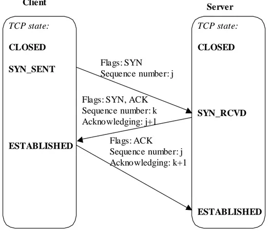
2.4.1 Three-Way Handshake

The TCP connection is set up using an algorithm called three-way handshake. It mostly works as shown in Figure 2-3. Client TCP state: CLOSED SYN_SENT ESTABLISHED Server TCP state: CLOSED SYN_RCVD ESTABLISHED Flags: SYN Sequence number: j Flags: SYN, ACK

Sequence number: k Acknowledging: j+1 Flags: ACK

Sequence number: j Acknowledging: k+1

Figure 2-3 – TCP three-way handshake

The client sends a segment, optionally including user data, with the SYN (synchronize) TCP header bit set. The server responds with a segment that acknowledges the received segment and also has the SYN bit set. Note that the SYN bit is counted as an octet of data, which will allow TCP to acknowledge a segment with a SYN bit with no real data using its ordinary ACK header field. When the client has received the server’s SYN segment and successfully acknowledged it, the connection is established on both sides.

In the figure, numbers j and k are chosen using a clock-driven algorithm, minimizing the possibility of old segments that have been delayed in the network to arrive and be mixed up with the segments of the new connection.

The three-way handshake does not always look like this. For example, if no application on the server is listening to the port that the client is trying to connect to, the server should return a segment with the RST bit set, causing the client to abort the connection attempt. Also, if one of the segments is lost during connection establishment it must be retransmitted using the

retransmission timer.

Yet another possibility is that both sides will try to connect (actively open) at the same time. This works fine, although the notion of TCP client and server is lost in that case.

2.4.2 Symmetric Release

The algorithm for shutting down a TCP connection is called symmetric release, since it is best seen as a way to shut down a pair of simplex (one-way) connections independently of each other. The host that wishes to send no more data sends a segment with the FIN TCP header bit set. This bit is, like the SYN bit, also counted as a bit of data. When the FIN segment has been acknowledged that direction of the connection has been closed.

The other direction will still be open and may be used for (in the first closers perspective) receiving data. The shutdown of the other direction will work in the same way. It is also possible that both sides will try to close simultaneously, which will also work.

The shutdown of a connection includes the TIME_WAIT state, which exists to give old

segments time to leave the network before another connection between the same two hosts and ports (sockets) can be established. The wait time is two times the estimated maximum segment lifetime (MSL) for the network, which equals to 2*120 seconds. However, if special

precautions are taken (given by [22]), a connection can be reopened (using the three-way handshake) from TIME_WAIT. The waiting time is sometimes confusing to the user of a TCP implementation, because his servers will refuse to restart before the waiting time is up.

2.5 TCP Options

The TCP options can be used to implement features that are not part of the original TCP specification without breaking backward compability. By setting the header length field to something above five (a TCP header without options is five 32-bit words) the user can send up to 40 octets of TCP option data. (The header length field is four bits wide and 15*32 bits – 5*32 bits = 40 octets.). The option consists of either a single octet that is an option identifier or one byte octet option identifier plus one octet of option length plus octets of option data. Because the header length is given in a number of 32-bit words, the option space that isn’t used has to be padded with zeros.

Below, three commonly used TCP options are explained. The more complicated SACK/DSACK options are explained in sections 2.6.5 and 2.6.6.

2.5.1 Maximum Segment Size (MSS) Option

This is the only option (besides the end of options list and the no operation options) specified in the original TCP specification. It is used by a TCP to tell the peer the maximum size of

segment that it is prepared to receive. This negotiating mostly happens during the three-way handshake when the option is included in the first segment that is sent from each side (that with the SYN bit set). If no MSS option is received TCP falls back to sending segments of the default size of 536 octets data. The segment size field is 16 bits wide, allowing segments to be up to 64 KBytes. Note that this is the same size as the maximum advertised window size. See [22] for details and a discussion of how the segment size affects performance together with IP.

2.5.2 Window Scale Option

The advertised window is limited to 64 KByte by the original TCP specification because the advertised window header field is only 16 bits wide. That is a problem on networks with a large bandwidth*delay product. The product is a measurement of how much data that must be outstanding (in transit in the network) to get full throughput. One example is a 100 Mbit

network with a RTT of 10 ms. The bandwidth*delay product is (10^8)/8 bytes/second * 10^-2 seconds = 125 KBytes, which means that the network will only be used to about half of its full capacity with a single TCP connection without the window scale option.

A solution to the problem is given in [24] and is based on a TCP option with an eight-bit data field holding a scaling factor. The scaling is interpreted as how many times to binary left shift the advertised window field. The maximum number allowed is 14 which gives an advertised window of 2^16 * 2^14 = 1 GByte.

2.5.3 Timestamp Option

TCP in Long Fat Networks (LFN), i.e. networks with a large bandwidth*delay product, also has other problems. First, the 32-bit sequence numbers are quickly reused if lots of data is transmitted. In a Gigabit network it takes about 17 seconds to wrap around. This should be compared to the maximum segment lifetime (the time a TCP segment is assumed to remain in the network in the worst case), which is 120 seconds. The problem is that segments may be reordered by the network, making it possible for an old segment to undetected be accepted as new data after the sequence number has wrapped around.

Secondly, the RTT sampling in a standard TCP implementation only occurs about once every RTT seconds. If the throughput is high, only a very small fraction of the segments are sampled. This may lead to poor quality in the RTO calculation. It is desirable to measure RTT for every segment, except retransmitted segments. Instead of keeping a list of all outstanding segments and the times when they were sent, the idea is to keep a 32-bit timestamp in the segment itself. The timestamp is then echoed by the receiving TCP, which also sends back a timestamp of its own. All the TCP needs to do to get the RTT is to subtract the timestamp time from the current time.

The real time clock that records the timestamps ticks much slower than the sequence numbers change, perhaps once every millisecond. The receiver can use both the timestamp and the sequence number to determine if the segment is old or new. This way the first problem is also solved using the timestamp mechanism.

2.6 TCP Congestion Control

Early TCP implementations relied only on the receivers advertised window when limiting the amount of data to send. The result was that TCP sent too much data into the network causing routers to be overloaded. When routers don’t have room for more packets in their input buffers (queues), they have to drop segments, causing a timeout in TCP. After the timeout TCP starts sending a lot of data again, overloading the network. Overload in a network is called

congestion. A number of new TCP mechanisms were suggested (in [36]) to deal with this problem. They were called congestion avoidance, slow start, fast recovery and fast retransmit and were standardized in [29]. These methods and several others are described below. Note that TCP assumes that all segment losses are caused by congestion.

To limit TCP’s aggressive behavior, implementations are required to keep a congestion window (cwnd) variable for each connection. The minimum of the cwnd and the receivers advertised window is used to limit the amount of outstanding data.

2.6.1 Congestion Avoidance

To utilize available bandwidth the cwnd is increased with one full sized segment every RTT. In practice it is actually done by increasing it by MSS*(MSS/cwnd) every time an

acknowledgement is received, because about (cwnd/MSS) acknowledgements will arrive every RTT. This is called addititive increase and is a conservative way to investigate the available bandwidth in the network. When the TCP uses addititive increase it is said to be in congestion avoidance.

2.6.2 Slow Start

Congestion avoidance is too slow to use in the beginning of a connection. Instead an algorithm called slow start is used. Slow start uses an exponential growth in the amount of allowed outstanding data. For each acknowledgement that arrives, the cwnd is increased by one full sized segment. So, for every acknowledgement that is received (at least) two new segments will be sent into the network, one to replace the segment that just left the network and one to use the increased cwnd.

Slow start is continued until the amount of outstanding data reaches the slow start threshold (ssthresh). This value may be arbitrary high, but is often set to the amount of the receivers advertised window [22]. When slow start is discontinued, the connection goes into congestion avoidance.

2.6.3 Retransmission Timeouts

The data sender discovers network congestion when the retransmission timer expires. To protect the network the data sender sets ssthresh to half the amount of outstanding data (which may be much lower than the current cwnd if the sender is limited by the receivers advertised window). This is called multiplicative decrease.

The cwnd is set to one segment (the ‘loss window’), which means that TCP goes back to slow start (because cwnd is now lower than ssthresh).

Also, the RTO value is doubled and the earliest segment not yet acknowledged is retransmitted, as outlined in section 2.3.

2.6.4 (NewReno) Fast retransmit and Fast Recovery

Retransmission timeouts was the only method early TCP implementations could use to

discover segment loss. This is clearly inefficient, as TCP first has to wait for the retransmission timeout and then go to slow start each time a segment is lost, even if it is only necessary to decrease the cwnd. The fast retransmit and fast recovery algorithms deals with these two problems. Both algorithms are often implemented together and because of that they are often treated as one.

Both sender and receiver are involved in the algorithms. The data receiver must send an

acknowledgment each time an out of order segment arrives and each time a segment that fills a hole in the input queue arrives.

The data sender can then look for ‘duplicate acknowledgements’, acknowledgements that acknowledges the same data over and over again. When an acknowledgement acknowledging the same data for the 4th time arrives, the sender can decide that the segment wasn’t just

reordered but actually lost in the network. The sender can then retransmit the lost segment (this is the fast retransmit). At the same time ssthresh is set to half the amount of outstanding data. When additional duplicate acknowledgements arrive, the congestion window is increased by one segment. This allows a new segment to be sent into the network. Later, when an

acknowledgement that acknowledges new data arrives, the congestion window is set to ssthresh. This means that the amount of outstanding data has been halved since the algorithm was started. By doing this, the network is protected and at the same time the penalty of going back to the loss window and slow start is avoided. This is the fast recovery part of the

algorithm.

If a timeout occurs during fast retransmit/recovery TCP still has to follow the rules from section 2.6.3.

Unfortunately, this algorithm does not work well when multiple segments are dropped from one window of data, since it will never retransmit more than one segment. This was discovered in [37] and one of the solutions proposed was the NewReno fast retransmit algorithm [30]. It works pretty much like the ordinary fast retransmit, except that it also uses ‘partial

acknowledgements’. When the algorithm is entered the highest sent sequence number is recorded into the send_high variable. When new data is acknowledged (but not up to

send_high) it is called a partial acknowledgement. The partial acknowledgement is taken as a sign of another segment loss and triggers another retransmission. The algorithm is exited when the data covered by the send_high sequence number has been acknowledged. The congestion window is decreased just like in the original algorithm.

NewReno fast retransmit/recovery comes in two flavors. The impatient one that does not reset the retransmission timer when a partial acknowledgement arrives and the slow but steady variant that does. The impatient variant does not give fast retransmit much of a chance to recover when the RTO value is not much larger than the RTT. The slow but steady variant can remain in fast retransmit/recovery for a very long time.

2.6.5 Selective Acknowledgement (SACK)

For each segment that has been lost, it takes at least one RTT for fast retransmit to discover the loss, since it only uses the acknowledgment field in the TCP header. To improve this, selective acknowledgements were invented. It uses a TCP option to negotiate if the connection is SACK capable during three-way handshake and then another TCP option to send additional

acknowledgements.

The SACK option can acknowledge up to four contiguous blocks of received data, which means it can send a negative acknowledgement of the same size. If other TCP options are used at the same time, less space will be available for SACK in the TCP header.

The specification [26] does not specify exactly when the sender should retransmit data based on SACK information, but it states that standardized congestion control mechanisms must be preserved. Especially, single duplicate acknowledgements must not cause retransmissions (the network may have reordered data segments) and the number of segments retransmitted in response to each SACK must be limited. This means that the fast recovery/fast retransmit algorithms are still useful in SACK implementations. Also, all TCP implementations are not SACK capable, so SACK capable implementations should work together with non-SACK implementations using fast recovery/retransmit.

The two major advantages with SACK over fast retransmit is that SACK can retransmit several segments without waiting a full round trip time and that it can retransmit the same segment several times.

2.6.6 Duplicate Selective Acknowledgement (D-SACK)

The D-SACK option is an extension to SACK specified in [27]. It deals with the sending of SACK segments when the receiver has received duplicate data segments. The idea is to give extra information to the data sender for more ‘robust operation in an environment of reordered packets, ACK loss, packet replication, and/or early retransmit timeouts’. D-SACK is backward compatible with SACK.

2.6.7 Limited Transmit

NewReno and standard fast recovery/retransmit is not efficient when the window size is small because not enough duplicate acknowledgments will arrive to the data sender. The same applies to SACK that needs some indication that segments have not just been reordered. Limited transmit [33] is an effort to solve the problem. It works by sending additional data when three acknowledgements for the same data has arrived, allowing the receiver to send additional duplicate acknowledgements that will trigger SACK retransmissions or fast retransmit/recovery. The additional data is sent providing that it is allowed by the receivers advertised window and that the new amount of outstanding data is not more than cwnd plus two segment sizes. The congestion window is not changed (that may be done later by fast recovery/retransmit). Note that the algorithm does not check that the congestion window actually is small.

2.6.8 Rate-Halving

Rate-halving [35] is another effort to react to congestion in the network. Rate-halving is a more advanced scheme than fast retransmit/fast recovery (see section 2.6.4) as it is designed to work together with both SACK (see section 2.6.5) and ECN (see section 2.7.3) as well as TCPs that uses duplicate acknowledgements to inform about congestion/loss of segments. It uses a finite state automata with four states that takes care of the three different kinds of congestion

notifications.

This makes the rate-halving algorithm a bit more complex than fast retransmit/recovery, but the benefit is that it makes better use of the available information about how much data that is in the network. Rate-halving includes an algorithm that was previously known as FACK (forward acknowledgement [40]) that uses the most recently SACKed data when determining the

amount of data that is in the network. The rate-halving algorithm also includes ideas similar to limited transmit (see section 2.6.7).

Another strength of the rate-halving algorithm is that it also uses all available information about which segments that have been received (also using SACK) when deciding on which segments to retransmit. By doing that it avoids some unnecessary retransmissions.

The rate halving-algorithm does not yet have its own RFC, but it is already in use on the Internet. It is the opinion of the author of this thesis that rate-halving has a good chance to become the most popular algorithm for TCP congestion control in the future, because it is the only algorithm available today that can use SACK and ECN information and still be

2.6.9 Automatic Receive Buffer Tuning

Researchers suggested this mechanism as a solution to the problem of achieving good

throughput in long fat networks. The idea is to dynamically increase the receive buffer and the advertised window to allow the sender to have more unacknowledged data outstanding in the network if the connection is made over an LFN. If the connection is made over an ordinary network, buffer space will be saved in the receiver.

The simple version of the algorithm is to increase the buffer when it is mostly empty; the more advanced one (described in [43]) is estimating the sender’s congestion window. There are no algorithms that save buffer space by ‘shrinking the window’, probably because [19]

discourages it. The reason is that sent data that can’t be received will cause retransmissions. Instead buffer tuning algorithms starts with a small advertised window and then increases them. The algorithm is not widely used but has at least been implemented in the Linux kernel.

2.6.10 TCP

Vegas

As described earlier, TCP uses segment losses to detect congestion. Some variants of TCP has gone one step further and also uses RTT measurements to detect build-ups of router queues. TCP Vegas [41] is the most famous of them (since it was actually implemented in a wide spread operating system, the 4.3 BSD Unix, nicknamed ‘Vegas’).

Vegas works by calculating the estimated throughput by dividing the congestion window size by the minimal measured RTT. Then it compares this number to the achieved sending rate, which is computed once per RTT. If the estimated value is close to the achieved value, the congestion window is increased, and if it is much lower than the estimated value the congestion window is decreased. The changes are done additively, not multiplicatively, since Vegas also uses fast retransmit and retransmission timeouts. The linear changes are only early changes in response to varying throughput.

2.7 Network Based Congestion Control

2.7.1 Drop-Tail Queue Management

Congestion appears when an Internet router’s input queue is filled and the router is forced to drop additional inbound IP packets. Just throwing away the last packet is called drop-tail queue management. This crude way of dealing with large amounts of traffic results in bursts of packet drops, maybe leading to loss of multiple segments from a single window, to which TCP is more sensitive than the loss of a single segment.

2.7.2 Random Early Detection (RED)

More advanced schemes have been proposed to deal with congestion. The first one discussed here is called Random Early Detection (RED) [42]. The purpose of RED is to implicitly inform the sender about congestion by dropping a segment, triggering the fast recovery algorithm (or retransmission plus slow start in TCP without fast recovery). Remember from section 2.6.4 that fast recovery halves the amount of allowed outstanding data and by that decreases network load. When the queue in the router has built up to a threshold value, the router starts dropping incoming packets with a probability that is calculated depending on the queue length.

2.7.3 Explicit Congestion Notification (ECN)

A related mechanism is called Explicit Congestion Notification (ECN) [34]. It has been proposed that it should use the same algorithm as RED, but instead of dropping the packet it will set the Congestion Experienced (CE) bit in the IPv4 header of packets that has the ECN-Capable Transport (ECT) bit set (this is the simple explanation, see the reference for a more accurate one).

TCP in the receiver will then inform the sender about the congestion by setting the ECN-Echo (ECE) bit in the TCP header in the TCP acknowledgement. The sender will then react as if the segment had been dropped (reducing the congestion window) and set the Congestion Window Reduced (CWR) bit in the next segment to acknowledge that it has received the ECE bit. ECN needs both the endpoints and the routers to participate in congestion avoidance. It also adds a fair amount of complexity to TCP endpoints, just for the benefit of not losing one segment. However, ECN is designed to be used with other transport protocols and can therefore become important in the future.

2.7.4 ICMP Source Quench

A fourth way that the network can trigger congestion avoidance in the TCP endpoints is by sending an ICMP source quench message to the sender. It is recommended by [22] that TCP should perform slow start upon the reception of such a message. This method is nowadays discouraged by [25] because it is regarded to be unfair and requires limitation in the number of source quench messages sent.

2.8 Other TCP Mechanisms

There is much more that deserves to be mentioned in a TCP overview than what has been mentioned here. However, only the TCP features mentioned above are discussed in the rest of this thesis. The rest of this chapter briefly explains some other TCP mechanisms that should be mentioned in an introduction to TCP. A lot of other suggested improvements for TCP have also been proposed, but are not discussed here. The most interesting reference that can be given is probably the ‘Long Thin Networks’ RFC [31], which deals with TCP over networks with long delay and low bandwidth. Please refer to the bibliography for more interesting reading.

Persist timer and window probes. When the receiver of data for some reason can’t read from

its buffers, the buffers will fill up and TCP will send out a segment that acknowledges all received data and sets the offered window to zero. When the user in the receiver reads from the buffers another (acknowledgment) segment with a window update will be sent to the data sender. There is no guarantee that the window update will not be lost in the network. To avoid a deadlock, the data sender uses a persist timer to send window probes, empty data segments, to the receiver. This gives the receiver a chance to send additional window updates or to tell the data sender that the window is still zero. The persist timer, like the retransmission timer, uses exponential back off. See [22] for details.

Keep-alive segments. This feature is sometimes included in TCP, but it is not required. It

checks if an idle connection is still valid by sending an empty data segment and wait for an acknowledgment. See [22] for details.

Silly Windows Syndrome (SWS). Early TCPs sent an acknowledgment segment with a

receiver window update every time a segment with data arrived. When the sender of the data got the acknowledgment back, it used the new window, even if the additional data that now

could be sent was a single byte. Currently TCP data receivers uses an algorithm found in [22] to avoid SWS. It simply says that the receiver should only change its’ advertised window if it can change it with a full sized segment (or with half its receive buffer if the buffer is smaller than two full sized segments). The SWS is described in detail in [20].

Nagle’s algorithm. The complementary problem to SWS is that TCP may send lots of small

segments instead of one large when data is given to TCP in small amounts. This gives a large overhead in the network since TCP/IP and other headers will be added to the data. The solution is to never automatically send data at once when the user gives it to TCP. Data is only sent when there is no unacknowledged outstanding data or when a full sized segment can be sent. The data is instead sent later, when an incoming acknowledgement changes the state of the system. Nagle describes his algorithm in [21].

Nagle’s algorithm is part of the sender side SWS avoidance algorithm. Another set of rules for when to send data is also defined in [22].

TCP/IP header compression for low-speed serial links. Jacobson describes how to increase

TCP/IP performance over serial links in [23]. The algorithm removes the TCP and IP header fields that are not changed during the lifetime of a connection and compresses the other fields. Compressed headers don’t work in a routed environment, since the IP addresses are removed from the IP packets. The compression decreases header size from 40 octets to five octets.

The GPRS Subsystem of GSM

3.1 The GSM System

Groupe Spécial Mobile that was formed in 1982 specified the GSM system. Some of the design goals were:

• Ability to support handheld terminals.

• Good subjective speech quality.

• Low terminal and service cost.

• Support for international roaming.

The GSM system (today interpreted as Global System for Mobile communications) has been tremendously successful and today has more than half a billion subscribers[8].

The GSM system is a cellular phone system, meaning that the geographical area that is covered by the system is divided into subareas called cells. Each cell site (a bunch of antennas)

generally covers three hexagon-shaped cells and the antennas are installed with a 120-degree angle between them. This is schematically shown in Figure 3-1.

3.2 GSM Nodes

To give the reader a basic view of how the GSM system works, here comes an explanation of the most important elements in a GSM system. Figure 3-3 on page 22 shows how the nodes are interconnected.

MS (Mobile Station): This is the handheld device itself, for example a GSM modem or a

phone. Among many other things, it contains a SIM (Subscriber Identity Module), which most notably contains a unique identity number and an encryption key.

BTS (Base Transceiver Station): The BTS is a relatively simple installation that has the

purpose of sending and receiving information to/from the MSs in one cell. It basically relays information between MS and BSC.

BSC (Base Station Controller): A BSC controls a number of BTSs. It manages handovers

(moving a MS from one cell to another), radio resources, frequency jumps and more. The BSC and a number of BTSs together are called a BSS (Base Station Subsystem).

MSC (Mobile Switching Center): The role of a MSC is to Connect BSCs to each other and to

the PSTN (Public Switched Telephone Network). It is the heart of the GSM system since it has the main responsibility for call routing.

HLR (Home Location Register): The HLR is a database containing static and dynamic

information about subscribers belonging to a certain MSC, for example where the MS is currently located.

VLR (Visitor Location Register): The VLR is often implemented together with the MSC. It

contains information about MSs that doesn’t belong in the associated MSC’s area. The VLR queries the HLR where the MS is registered if it should provide service to a visiting MS or not.

3.3 GSM Radio Interface

GSM is a FDMA (Frequency Division Multiple Access) system, meaning that the frequency spectrum that is used is divided into frequencies 200 kHz apart. Each cell uses one or more frequency pairs to transmit traffic. One of the frequencies in each pair is used for downlink (BTS to MS) traffic and the other for uplink (MS to BTS) traffic. The different shades of gray in Figure 3-1 shows how groups of frequencies can be assigned to cells so none of the adjacent cells use the same frequencies.

GSM is also a TDMA (Time Division Multiple Access) system. This is shown in Figure 3-2. Each frequency is used for up to eight simultaneous calls. The frequency is divided into small amounts of time, time slots, lasting for approximately 0.577 ms. The calls are broken into pieces and a small part of each call is sent in every eight time slot. Eight consecutive time slots are called a TDMA frame. 26 TDMA frames are forming a TDMA multiframe. Of the 26 frames in a multiframe 24 are used for traffic and one is used for management information, the last one being unused. When a call is made one time slot in each frame is reserved for that MS both on the downlink and the uplink frequency.

Frames 0-11: Data Frame 12: Management data Frames 13-24: Data Frame 25: Unused 23 22 21 20 19 18 17 16 15 14 13 12 11 10 9 8 7 6 5 4 3 2 1 0 24 25

TDMA 26-frame multiframe: 120 ms

0 1 2 3 4 5 6 7

TDMA frame: 60/13 ms

Time slot (burst): 15/26 ms

Figure 3-2 – TDMA in GSM

In GSM terminology the word channel should be used with care, since it may mean many things. A pair of uplink/downlink frequencies forms a radio channel. One reserved timeslot in every TDMA frame on a given frequency is a TDMA channel. In GPRS, it is even worse since many MSs may share the same TDMA channel, dividing it into other kinds of channels. Don’t worry; it is perfectly normal to be confused.

3.4 Data in the GSM system

In circuit switched GSM, the oldest way to transmit data is to use one time slot in each direction, just like when voice data is transmitted. The data rate in that case is 9.6 kbit/s or in newer systems 14.4 kbit/s. New technology, HSCSD (High Speed Circuit Switched Data), has been developed to use more time slots in order to get higher transfer rates. In theory it is possible to use all eight time slots of a frequency, but in practice only up to four time slots are used, quadrupling the transfer rate up to 57.6 kbit/s.

The disadvantage with the circuit switched data transfer technologies is that it uses radio resources even when no data is being sent, preventing other users from using them. Because of that it gets very expensive to stay online. As we will see below, GPRS makes an effort to solve that problem.

3.5 The GPRS Subsystem

As Internet usage grew rapidly in the 1990s, the demand for wireless access also increased. One of the new technologies that appeared was the General Packet Radio Service (GPRS). Some of the design goals for GPRS are:

• Provide a packet switched service, enabling access to the Internet or other external IP or X.25 networks.

• Use the existing GSM infrastructure and radio resources in an efficient way.

• Reduced cost for online time for end users.

• Enable QoS (Quality of Service) agreements for different traffic types.

• New, efficient coding schemes, modulation and multislot capabilities in the air interface providing relatively high data transfer rates.

• Allow devices that can send and receive voice and data simultaneously [10].

In order to introduce a packet switched service into the circuit switched GSM system, a number of changes has to be made. The following sections briefly describe the most important

additions to the original GSM.

3.6 Changes to the GSM Radio Interface

In circuit switched GSM a MS is always allocated one time slot on each of the uplink/downlink frequencies. GPRS allows dynamic and asymmetric allocation of radio resources and a MS with so called multislot capability can in some circumstances use all eight timeslots of a

frequency, but it can also be completely idle although still being connected to the network. The Medium Access Control (MAC) is therefore a lot more complex in GPRS. Even though a MS can use radio resources in an asymmetric way (i.e. receive more data than it sends) the total available bandwidth is equal in the uplink and downlink directions since the GSM scheme of using frequencies still apply.

In the physical layer GPRS uses GMSK, which is the same modulation as GSM uses. There are four Coding Schemes (CS) called CS-1 through CS-4. Each coding scheme adds a different amount of redundancy to the data and uses different parity checking. These coding schemes allow data rates between 9.05 and 21.4 Kbit/s per time slot used.

Enhanced GPRS (EGPRS) is an extension to GPRS that introduces a new modulation called 8-PSK into the GSM system. It also introduces nine new coding schemes called MCS-1 through MCS-9. EGPRS is the GPRS version of EDGE, which stands for Enhanced Data Rates for Global Evolution. EDGE technology is also used in other new mobile phone systems.

Table 3-1 shows the EGPRS coding schemes and the different data rates that can be achieved by using them. In the table, code rates for the different coding schemes and the resulting data rates are shown. A code rate of 1 means that no redundant information is sent with each packet, a code rate of 0,5 means that twice the amount of information that should be necessary to decode the message is sent and so on. The headers of the packets are coded separately because they need to be protected with more redundancy, which gives them a lower code rate.

Coding scheme Code rate Header Code Rate Modulation RLC blocks per Radio Block Raw Data within one Radio Block (bits)

Family Data rate Kbit/s MCS-9 1.0 0.36 2 2x592 A 59.2 MCS-8 0.92 0.36 2 2x544 A 54.4 MCS-7 0.76 0.36 2 2x448 B 44.8 MCS-6 0.49 1/3 1 592 A 29.6 MCS-5 0.37 1/3 8-PSK 1 448 B 24.4 MCS-4 1.0 0.53 1 352 C 17.6 MCS-3 0.8 0.53 1 296 A 14.8 MCS-2 0.66 0.53 1 224 B 11.2 MCS-1 0.53 0.53 GMSK 1 176 C 8.8

Table 3-1 – Coding schemes in EGPRS [1]

There are two ways of dealing with changing radio conditions in EGPRS, Link Adaption (LA) and Incremental Redundancy (IR). The purpose of LA is to be able to change to another coding scheme if the radio conditions change. If conditions are bad, a coding scheme with more redundancy can be used. This technology requires the MS to send reports of the quality of the received information back to the BSC.

IR works by retransmitting data. The output of the coder is two or three times the amount of bits that are really necessary to decode the message if all bits are transmitted correctly. If the message needs to be retransmitted, another version of the message is sent. All versions of the message are saved, until enough information to correctly decode the message is available. This makes IR more memory intensive than LA. IR and LA can be used together – if a RLC block is lost, it may be transmitted using another coding scheme (probably with a lower data rate) provided that the new coding scheme belongs to the same family (see the ‘family’ column of Table 3-1).

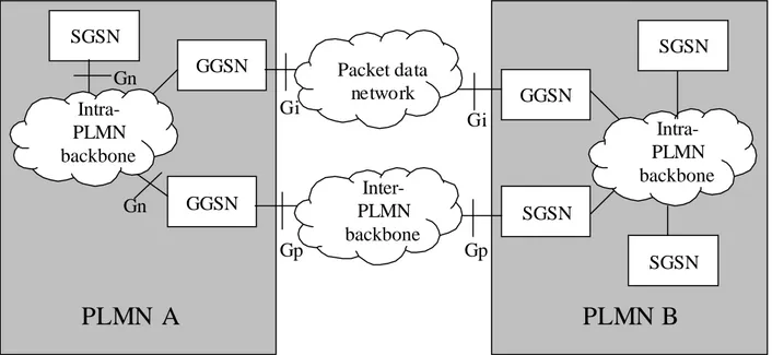
3.7 GPRS Nodes

To allow packet switched data in the GSM system, some entirely new nodes have to be installed. They may be implemented together as one physical unit or separately. Figure 3-3 shows where they belong in the GPRS network and Figure 3-4 gives a more detailed description about how the new nodes can be interconnected among themselves.

SGSN (Serving GPRS Support Node): The SGSN is responsible for keeping track of a MS in

the system. Therefore it also handles packet routing inside and between PLMNs (Public Land Mobile System, i.e. one operator’s GSM system is a PLMN). Security functions are also implemented here.

GGSN (Gateway GPRS Support Node): The task of a GGSN is simply to deliver packet data

Additionally, some of the existing nodes need to be updated to support GPRS. Most notably for the user is of course that he must have a new phone with GPRS or EGPRS capabilities if he wants to use the GPRS services. Other nodes also need to be updated, worth mentioning here is that a Packet Control Unit (PCU) is added to the BSC. It handles most of the things that chapter 5 of this thesis is dealing with.

Backbone IP network GGSN MSC/VLR SGSN GMSC BSC HLR GPRS register GGSN BTS MS External IP or X.25 network PSTN

MS Mobile Station SGSN Serving GPRS Support Node

BTS Base Transceiver Station GGSN Gateway GPRS Support Node

BSC Base Station Controller

MSC Mobile Switching Center HLR Home Location Register

GMSC Gateway Mobile Switching Center VLR Visitor Location Register

PSTN Public Switched Telephone Network

Figure 3-3 – The GPRS nodes [1] (very simplified)

GGSN GGSN SGSN Intra-PLMN backbone

PLMN A

PLMN B

3.8 The GPRS Protocol Stack

A lot of new protocols are required to allow transport of packet switched data through the GSM system. Figure 3-5 shows the entire protocol stack that is used for data transfers. The stack defines how data is treated when sent through the network. Each protocol (a box in the stacks) adds some control data to the user data when sending. When the corresponding protocol in another node in the network receives the data, that control data is checked and removed again. As an example we can see that the SNDCP protocol is used between MS and SGSN and the nodes between them sees the SNDCP control data only as any other user data.

Note that some of the protocols in Figure 3-5 are GPRS specific, some are also used in external networks and some (in the physical and data link layers) are not specified in the GPRS

standard. Application Network layer (IP, X.25) SNDCP LLC PLL RFL RLC MAC Phy. layer Network service Phys. layer GSL MS RLC/MAC GSL Phys. layer PLL RFL BSSGP BTS Data link layer

Um Abis Physical layer BSC GTP Data link layer TCP/UDP IP Phy. layer Phy. layer Data link layer IP TCP/UDP Network service BSSGP LLC SNDCP GGSN SGSN Gb Gn Gi GTP Network layer (IP, X.25) Phy. layer Relay Relay Relay

SNDCP Subnet Dependent Convergence Protocol BSSGP BSS GPRS Application Protocol LLC Logical Link Layer GSL Global Service Logic RLC Radio Link Control GTP GPRS Tunneling Protocol MAC Medium Access Control TCP Transmission Control Protocol PLL Physical Link Layer UDP User Datagram Protocol RFL Physical RF Layer IP Internet Protocol

Figure 3-5 – GPRS protocol architecture [1]

The following sections contain a short overview of the different protocols involved. They are presented using the OSI reference model, with some missing layers excluded. The

specifications of the GPRS specific protocols can be found in [12], [14], [15], [16] and [17].

3.8.1 Application Layer

Most existing networked applications, like HTTP, FTP and mail clients, are supposed to work on a GPRS enabled host. The only requirement is that they use an API based on a supported network layer protocol, preferably IPv4.

3.8.2 Transport Layer

As with the application layer, the only requirement for the transport protocols used with GPRS is that it works with a supported network layer protocol. In practice, TCP and UDP (User Datagram Protocol) are the common cases. Note that the transport layer isn’t visible in Figure 3-5, since it is not part of the GPRS specification.

3.8.3 Network Layer

IP and X.25: GPRS is designed to be able to relay data to both external IP and X.25 networks.

In practice however, only IP will be used in most cases, and only to access one external network, the Internet. The GPRS system is designed to be able to support IPv6 capable hosts.

SNDCP (Subnetwork Dependent Convergence Protocol): The main role of SNDCP is to

encapsulate IP and X.25 packets so that both can be transported through the GPRS system. SNDCP also performs TCP/IP header compression (see section 2.8). Optionally SNDCP also uses V.42bis data compression [46] on the entire data content, including the compressed TCP/IP headers. SNDCP is used between MS and SGSN.

3.8.4 Data Link Layer

LLC (Logical Link Control protocol): The purpose of LLC is to provide a logical link between

an MS and a SGSN. LLC can be used in both acknowledged and unacknowledged mode. In acknowledged mode, it provides in-order delivery and error recovery. This may be desired if the lower-level protocols used (GPRS doesn’t define them) lack such features (e.g. Frame Relay). In practice LLC will probably be used in unacknowledged mode since the links

between BSS (Base Station Subsystem) and SGSN are supposed to be almost error-free and the air interface uses the recovery features of RLC/MAC.

Additionally LLC always provides a 24-bit CRC (Cyclic Redundancy Check) code and

ciphering. The ciphering is necessary to avoid eavesdropping in the air interface. Furthermore, SMS (Short Message Service) uses the services of LLC.

RLC/MAC (Radio Link Control and Medium Access Control protocol): This is the most

complex protocol in the GPRS system. Chapter 5 of this thesis is heavily focused on RLC/MAC, so it is given more attention here than the other protocols.

The RLC part of the protocol handles the logical link between MS and BSC. The link can be run in either acknowledged or unacknowledged mode, but because the radio interface is so unreliable acknowledged mode is preferred since bandwidth and time would be lost if higher-level protocols were used to retransmit data. The RLC layer is also responsible for the Link Adaption scheme. If the connection is in acknowledged mode, Incremental Redundancy may be used (see section 3.6 for an explanation of LA and IR). RLC also uses a Negative

Acknowledgment (NACK) scheme to tell the peer which RLC blocks that wasn’t decoded correctly and must be retransmitted. Like TCP, RLC is a sliding window protocol.

A connection in the MAC part of the protocol is called a Temporary Block Flow (TBF). The TBF is a unidirectional connection, which is set up when the MS or the BSC needs to send data. The radio resources are managed by the PCU in the BSC, so a downlink TBF can be established once the PCU has the radio resources it needs to send data. The MS however, must first request to be assigned radio resources before it can send anything. For this, a special channel, called Master Packet Data Channel is used.