Material modelling for simulation of heat treatment

Full text

(1)2003:07. LICENTIATE THESIS Material Modelling for Simulation of Heat Treatment. Henrik Alberg. Licentiate Thesis Department of Applied Physics and Mechanical Engineering Division of Computer Aided Design. 2003:07 - ISSN: 1402-1757 - ISRN: LTU-LIC--03/07--SE.

(2) II.

(3) Preface This research has been carried out at Computer Aided Design at Luleå University of Technology in close cooperation with Volvo Aero in Trollhättan, where my workplace is. I would like to thank my supervisor Professor Lars-Erik Lindgren for all discussions, the critical review of my work and for your great enthusiasm. Thank you Lars-Erik! I would also like to thank Dr. Henrik Runnemalm at Volvo Aero who has made it possible for me to work in Trollhättan and for the discussion and advises. Thank you Henrik! Daniel Berglund, my colleague and co-author for two papers. Thank you Daniel for the encouragement in the beginning of my research, the discussions, advises and nevertheless all the laughs! The financial support has been provided by the MMFSC1-project a European Union funded project within the 5th framework and Luleå University of Technology. All are gratefully acknowledge. My daily work has been carried out at the division of Advanced Manufacturing Technology at Volvo Aero. I would like to thank all persons at the division for a good working environment and for sharing the your knowledge in many different areas. A special thanks to the simulation group for the many good discussions and ideas. Finally but not the less I would like to thank my girlfriend Viktoria Rönnqvist for all encouragement, happiness and for just being you. Thank you Viktoria you are the best!. Henrik Alberg Trollhättan, January 2003. 1. Manufacturing and Modelling of Fabricated Structural Components III.

(4) IV.

(5) Abstract Heat treatment of materials is a fundamental metallurgical process. Materials are subjected to heat treatment to relieve internal stresses, reduce brittleness and to improve machinability. The properties of materials can also be altered such as hardness, strength, toughness, and wear resistance to suit particular applications. Nevertheless, heat treatment can generate unwanted stresses and deformations, a fact that has to be taken into consideration when designing or changing the sequence of manufacturing for a given component. One way to decrease cost and reduce time in product development can be to use simulation tools that can reliably predict the final properties and shape of a component caused by the used manufacturing process. A decrease in cost and better knowledge of final properties already in product development can give the company a better market position and competitiveness. The objective of the work presented in this thesis is to develop efficient and reliable methods and models for simulation of heat treatment using the Finite Elements Method. The result of the simulation must be sufficiently accurate and completed within an acceptable time when the manufacturing simulation is to be used in product development. The models would enable us to predict residual stresses, distortion, final shape, and amount material phases after a heat treatment process. The formulation of constitutive equations for elasticity, plasticity, and creep is discussed, along with three unified models, bringing together plasticity/viscoplasticity, and creep into one model. There are many materials models to choose among but material parameters are usually lacking. An approach where the same numerical algorithm for the implementation of a constitutive model in the finite element code is also used for material parameter identification is presented. A parameter fitting using a viscoplastic model with nonlinear isotropic hardening is performed. Combined welding and heat treatment simulation is performed on a geometrical complex shaped aerospace component. Efforts to accurately determine the boundary conditions have been made. During the cooling sequence most of the heat transfer is carried out by convective heat transfer. Therefore, a method is developed and a CFD analysis is carried out to obtain this convective heat transfer. Moreover, comparisons how the use of different material models affects the response from combined welding and heat treatment on an aerospace component is made. The material models include different effects; rate-independent and viscoplastic models including microstructure calculation and transformation induced plasticity. Different creep models and different ways to apply them have also been investigated.. Keywords Manufacturing simulation, Finite Element Method, Heat treatment, Constitutive model. V.

(6) VI.

(7) Contents 1. INTRODUCTION. 1. 2. SCOPE OF WORK. 1. 2.1 2.2. 3 3.1 3.2 3.3 3.4. 4 4.1 4.2. Simulation of heat treatment Heat Treatment of Metals. 1 2. CONSTITUTIVE MODELLING. 6. Rate-Independent Plasticity Rate-Dependent Plasticity (Viscoplasticity) Unified plasticity models Parameter Optimisation. 6 7 9 9. MODELLING OF HEAT TREATMENT. 12. Modelling of Material Behaviour Modelling of Thermal Boundary Conditions. 12 15. 5. SUMMARY OF APPENDED PAPERS. 19. 6. DISCUSSIONS AND FUTURE WORK. 20. APPENDED PAPER PAPER A. D. Berglund, H. Alberg, and H. Runnemalm Simulation of Welding and Stress Relief Heat Treatment of an Aerospace Component, accepted for publication in Finite Element in Analysis and Design. PAPER B. L-E. Lindgren, H. Alberg, and K. Domkin Constitutive Modelling and Parameter Optimisation, accepted for presentation at VII International Conference on Computational Plasticity.. PAPER C. H. Alberg and D. Berglund Comparison of plastic, viscoplastic, and creep models in modelling of welding and stress relief heat treatment, submitted for publication. VII.

(8) VIII.

(9) Henrik Alberg – Material Modelling for Simulation of Heat Treatment. 1. Introduction. Heat treatment of materials is a fundamental metallurgical process, which dates back thousands of years. The earliest evidence of heat treatment was on a dagger, which had been forged and tempered in Egypt around 1350 BC. The blacksmiths’ art had its foundations in the Iron Age and for centuries, blacksmiths have used heat in the manufacture of armour, tools, and many other metal objects. Materials can be subjected to heat treatment to relieve internal stresses, reduce brittleness and to improve machinability. Properties of materials such as hardness, strength, toughness, and wear resistance can be changed to suit particular applications. The basic principle involved in heat treatment is simply the process of heating and cooling. In steel for example, hardness is achieved by heating and cooling rapidly. Heating and slowly cooling will relieve internal stresses in many materials. Nevertheless, the underlying microstructural changes induced in materials during heat treatment are complex. In the aerospace industry, heat treatment is usually performed after welding or forming. A desire to understand and to control the heat treatment process is the motivation for the research performed in this thesis. The content in this thesis can be divided into four parts. The first part reviews earlier work made in the topic. A description of the heat treatment process and equipment will be made along the active physical process during the different heat treatment processes. Secondly, constitutive equation for metal rate-independent plasticity, viscoplasticity, and creep are examined. Material models unifying plasticity/viscoplasticity and creep into the same model, called unified models is reviewed. Although the existence of many constitutive models, a common problem is that material parameters are lacking. An approach where the same numerical implementation of a constitutive model to be used in the finite element code, also is used for material parameter identification, will be presented. The third part describing the modelling of the heat treatment process. This part considers material models and boundary conditions used in heat treatment simulations. Finally, part four presents a summary of the appended papers, together with conclusions and a discussion of future work.. 2. Scope of work. The objective of the work is to develop an efficient and reliable method for simulation of heat treatment using finite element analysis. The simulation can then be used for designing and planning the manufacturing process in order to obtain an adequate final shape of the component and a robust manufacturing process. The result of the simulation must be sufficiently accurate and completed within an acceptable time when the manufacturing simulation is to be used in product development. This requires simplifications of the model; correct modelling of boundary condition, and material behaviour for the process. The work presented in this thesis is focusing on the question about reliability of the models because of uncertainties in boundary conditions and material behaviour.. 2.1. Simulation of heat treatment. Heat treatment can generate unwanted stresses and deformations, a fact that has to be taken into consideration when designing or changing the sequence of manufacturing for a given component. Previous experience can offer some help but costly and time-consuming experiments are often required to evaluate component design, material selection, and manufacturing schedules. One way to decrease cost and reduce time in product development can be to use simulation tools that can 1.

(10) Henrik Alberg – Material Modelling for Simulation of Heat Treatment reliably predict the final properties and shape of a component caused by the used manufacturing process. A decrease in cost and better knowledge of final properties already in the product development stage can give the company a better market position and competitiveness. The objective of heat treatment simulation studies is to establish a predictive theory that would enable us to predict residual stresses, distortion, and material properties such as microstructure of material and hardness after a heat treatment process. To be able to improve a heat treatment process it is important to understand the material behaviour and to control the process parameters. One frequently used numerical method to simulate thermo-mechanical behaviour is the Finite Element Method (FEM). FEM has been used since the beginning of the 1970’s in analysis of thermo-mechanical manufacturing processes such as welding, Hibbit et al. [1], and Ueda et al. [2]. Simulation of heat treatment has also been made since the 1970’s. Early heat treatment simulations were carried out by Burnett et al. [3]. Burnett et al. calculated residual stresses in case-hardened cylinders. Sjöström [4] calculated quench stresses in steel. Rammerstorfer et al. [5] made simulation of the heat treatment process, which included creep and phase changes. During the last two decades, most of the heat treatment simulations have been made to solve quenching problems. The primary intends with that simulations have been to predict distortion and residual stresses. Donzella et al. [6] predicted the residual stresses and microstructure in a solid rail wheel. Thuvander [7] made simulation of distortion due to quenching. Simulation tools have also been developed to calculate hardness after quenching, Tajima [8]. Simulation combining quenching and tempering are performed by for example, Ju et al. [9]. Simulations of stress relief heat treatment are less common. Josefson [10] calculated the residual stresses after in a stress relief heat treatment of a thin wall pipe. In this thesis, simulation of heat treatment is carried out with the Finite Element Method. In Paper A and Paper C, stress relief heat treatment has been simulated to reduce stresses after welding. It seems like combined welding and heat treatment simulations are not very common. Nevertheless, combined simulation has been performed by Josefson [10] who calculated the residual stresses after post weld heat treatment of a thin wall pipe. Wang et al. [11] simulated local post heat treatment of a pipe with different heated bands and used a power creep law when simulating the stress relaxation.. 2.2. Heat Treatment of Metals. Heat treatment is a collection of many processes such as annealing, stress relief, quenching, tempering, and ageing. All the different heat treatment processes consists the following three stages 1) heating of the material, 2) holding the temperature for a time, and 3) cooling, usually to room. However, the temperature and time for the various processes is dependent on the material mechanism controlling the wanted effect. For example, if the driving mechanism is diffusional the time must be long enough to allow any necessary transformation reaction. During heating and cooling, there exist temperature gradients between the outside and interior portion of the material; their magnitudes depend on the size and geometry of the workpiece. If the rate of temperature change in the surrounding is too high, large temperature gradients may develop in the component. This creates internal stresses that may lead to plastic deformations and even to cracking. The description of the heat treatment processes presented in this chapter is mainly based on the books in material science by Shackelford [12] and Callister [13].. 2.

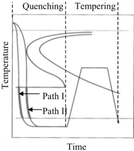
(11) Henrik Alberg – Material Modelling for Simulation of Heat Treatment. 2.2.1. Annealing. Annealing is typically carried out to relieve stresses, increase softness, ductility, toughness, to produce a specific microstructure and/or negate the effects of cold work. In annealing the material is exposed to an elevated temperature for a time and then slowly cooled. This procedure is the same for all processes in this section. The annealing temperature is roughly one-third of the melting temperature for a pure metal. For alloys, the temperature can be as high as one-seventh of the melting temperature. Since atomic diffusional processes normally are involved in annealing, the temperature and time are important parameters. The mechanism active during annealing is recovery and recrystallisation. Grain growth is generally not allowed to occur. Further reading regarding recovery, recrystallisation, and grain growth can be found in Shackelford [12], Callister [13], and Stouffer et al. [14]. Stress relief heat treatment is an annealing process where the aim is to reduce residual stresses. The material is usually heated to a temperature below the annealing temperature. The material is kept at this temperature long enough to attain the desired stress relief. Creep is the main active physical process in stress relieving. Creep is active already at room temperature, but an increase in temperature implies increase the creep rate. Creep is a composition of many processes on atomic level where thermal activated processes like diffusion play important parts, Stouffer et al. [14].. 2.2.2. Hardening Processes. In this section, two different techniques to obtain a harder and/or less ductile material will be discussed. The two different techniques are often referred to as quenching and precipitation hardening. Their different procedures are due to different active physical processes.. Path II. Temperature [F]. Temperature [°C]. In quenching, the material is rapidly cooled to obtain a special microstructure. For example, steel (<2.0wt%C) is heated to form austenite. If the material is cooled fast enough, all austenite will form martensite, Path I in Figure 1. If the material is cooled slower a mixture of pearlite, bainite, and martensite will form, Path II in Figure 1. The martensitic transformation is a diffusionless transformation that involves a sudden reorientation in the material structure.. A -Autenite P - Pearlite B - Bainite M - Martensite. Path I Time [s]. Figure 1. TTT-diagram for steel. Path I – complete formation of martensite. Path II – formation of pearlite and bainite. 3.

(12) Henrik Alberg – Material Modelling for Simulation of Heat Treatment Martensite is a hard, brittle phase, in fact so brittle that a product of 100% martensite would be impractical. A common approach to reduce this is therefore to reheat carefully to a temperature to form equilibrium phases such as α−Fe and Fe3C. This process is called tempering, Figure 2. Tempering is associated with a decrease in hardness and increase in ductility. A possible problem with conventional quenching and tempering is that the exterior of the workpiece will cool faster than the interior. Therefore, will the exterior transform to martensite before the interior, Figure 2. During the period of time in which the exterior and interior have different crystal structures, significant stresses may occur, the result may be distortions and cracks. The problem can be solved using heat treatments known as martempering and austempering, which can be found in books in material science, Shackelford [12], or Callister [13]. Tempering. Temperature. Quenching. Path I Path II. Time. Figure 2. TTT-diagram for showing the tempering. Path I is the temperature in the inner of the component. Path II is the temperature in the outer of the component. The strength and hardness of some metal alloys, for example titanium or nickel-base alloys, may be enhanced by formation of small uniformly dispersed particles of a second phase within the original material phase matrix. This is accomplished by a heat treatment called precipitation hardening or age hardening. Precipitation hardening and the quenching-tempering of steel are different phenomena, although the heat treatment procedures are similar. Precipitation hardening is accomplished by two different heat treatments, Figure 3a. The first is a solution heat treatment in which all solute atoms (precipitants) are dissolved to form a single-phase solid solution. When the solid solution has a single phase, the material is cooled rapidly, usually to room temperature. Due to this rapid cooling, the diffusional effects accompanying the transformation effect to the second phase are prohibited and the material stays single-phased. At this state, the material is usually soft and weak. The second step in the precipitation hardening is ageing. The solid-solution is heated to a temperature where diffusion rates for the second phase become appreciable. The ageing temperature is lower the temperature used for solution heat treatment. During the ageing process, the second phase begins to form finely dispersed particles. These precipitants are effective dislocation barriers and lead to substantial hardening of the alloy. After appropriate ageing time, the material is cooled. If the ageing process are continued so long that the precipitates have an opportunity to coalesce into a more coarse dispersion, a less effective dislocation barrier will form, this is called overageing, Figure 3b.. 4.

(13) tageing. a). Time. Yield stress. Temperature. Henrik Alberg – Material Modelling for Simulation of Heat Treatment. Time. b). Figure 3. a) The participation hardening process. b) Overageing. 2.2.3. The Heat Treatment Process. The heat treatment process studied in the current work is described below. The equipment used for heat treatment is shown and the different sequences during heat treatment are presented. A common heat treat equipment is a vacuum furnace, Figure 4, with an operating pressure of about 10-5 to 10-3 of the atmospheric pressure. In vacuum heat treating the metal is heated in a heated enclosure that is evacuated. Vacuum can sometimes be substituted for a protective gas during a part or all parts of the heat treatment. Vacuum furnaces are used for many types of heat treatment processes such as, annealing, nitriding, carburising, quenching, tempering, stress relieving and ageing. These types of furnaces have high flexibility and are comparably friendly to the environment. Further reasons to use vacuum furnaces are to prevent surface reactions, such as oxidation or decarburisation, on the workpieces, thus retain a clean surface intact. Radiator. Charge volume Grid / Plate. Component Inlet / Outlet. Fan. Figure 4. Exploded view of a vacuum furnace. In the heating sequence, the component is heated by radiators, Figure 4. To obtain a more even heating of the material a gas may be present, i.e. heating by convection. During the cooling sequence, gas is pumped into the charge volume from an external vessel. The gas enters through holes in the top, side and/or through holes in the bottom. The inlet and outlet may be altered to obtain an even cooling of the component. The cooling gas is subsequently recirculated until the component reaches room temperature. More information regarding the heat treatment equipment and the different heat treatment processes can be found in ASM Handbook on Heat Treating [15] 5.

(14) Henrik Alberg – Material Modelling for Simulation of Heat Treatment. 3. Constitutive Modelling. This chapter deals with the formulation of constitutive equations for elasticity, rate-independent plasticity, and rate-dependent plasticity (viscoplasticity). Material models unifying plasticity/viscoplasticity and creep into the same model, called unified models is reviewed. Although the existence of many constitutive models, a common problem is that material parameters are lacking. Later in this chapter a presentation of a combined approach where a numerical implementation of a constitutive model in a finite element code is used for material parameter identification. For many metals the models for plasticity depend on shear stress and are independent of mean stress or hydrostatic stress, i.e. deviatoric models. It has also been observed that inelastic deformation does not produce a significant increase in volume. These two effects together with the basic equations of thermodynamics are important in the development of constitutive models for plasticity. The material models described and used in this thesis are based on deviatoric plasticity. The thermodynamic treatment will be omitted here, but can be found in for example in Lemaitre et al. [16]. Books discussing different phenomena and models in plasticity are the Lemaitre et al. [16], Miller [17], and Stouffer et al. [14]. The models are ranging from the deviatoric, ideal or nonlinear plasticity model using von Mises yield condition and the associated flow rule to complex set of equations like the MATMOD-model, Miller [17]. The formulation of constitutive equations for finite deformation metal rate-independent plasticity and viscoplasticity is based on assuming additive decomposition of the strain rates and the use of a hypoelastic stress-strain relation. The assumption of additive decomposition of the strain rates, discussed in Belytschko et al. [18], is used. Thus,. ε&ij = ε&ije + ε&ijp + ε&ijth + ε&ijtr + ε&ijtp. (1). ε&ij is the total strain rate, ε is the elastic strain rate, ε is the plastic strain rate, ε is thermal strain &ije. &ijp. &ijth. rate, ε&ijtr is the transformation strain rate, and ε&ijtp is the rate of transformation induced plasticity strain. A multiplicative split of the strain rate is possible and is discussed by Simo et al. [19]. The material models used in this thesis, no difference between the inelasticity from rate-independent plasticity, rate-dependent plasticity, or creep. Thus, all these contributions are collected in the plastic strain term. A hypoelastic relation is used where Hooke’s law gives the stress rate due to an elastic strain rate. The hypoelastic model and assumed additive decomposition of strain rates gives, tp th tr σ& ij = Cijkl ε&kle = Cijkl ε&kl − ε&klp − ε&kl (2) − ε&kl − ε&kl. (. ). Where Cijkl is the elasticity tensor and σ& ij is an objective stress rate. Constitutive models for plasticity and viscoplasticity will be considered below. These models share the same assumption about the elastic behaviour of the material.. 3.1. Rate-Independent Plasticity. Three fundamental concepts in rate-independent plasticity, in this thesis referred to as plasticity, are the yield surface or yield criterion, the flow rule, and the hardening rule. The yield criterion or yield surface determines when plastic flow occurs. The flow rule stating, how the plastic flow occurs. The hardening rule stating the evolution of the yield surface. A fundamental requirement in plasticity is that the stress state never can be outside the yield surface. A stress state inside the yield surface implies an elastic process and a stress state on the yield surface implies plastic process. Hence, the following yield surface is formulated, 6.

(15) Henrik Alberg – Material Modelling for Simulation of Heat Treatment  < 0 elastic process f = σ −σ y  (3) ≡ 0 plastic process Where σ is the effective stress defining the stress state, Equation 4a and b, and σy is the yield limit. The yield limit is usually dependent on temperature and its evolution is dependent on the hardening, discussed below.. (. )(. ). σ 3 s − α ij sij − α ij sij = σ ij − kk δ ij (4a, b) 2 ij 3 sij is the deviatoric stress tensor, defined in Equation 4b and αij is the back stress tensor due to kinematic hardening. The hardening behaviour of the material discussed here has an isotropic and a kinematic part. The first is accounted for by the change in size of the yield surface of the material and the latter by translating the yield surface, i.e. changing the backstress. Both types of hardening may also include terms for recovery effects, omitted here. Equation 5a defines the linear isotropic hardening and Equation 5b defines linear kinematic hardening. However, there exist many different equations to describe the hardening. σ =. σ y = σ y 0 (T ) + H ′(T )ε. α ij = C (T )ε ijp. p. (5a, b). H’ and C are material parameters. Due to the requirement of maximum dissipated energy from the thermodynamics, the plastic flow is assumed orthogonal to the yield surface, associated plasticity. ∂f 3 ε&ijp = λ& = ε& p s ij (6) 2σ ∂σ ij λ& is the plastic multiplier, the associated flow rule is used throughout this thesis The effective. plastic strain rate, ε& p , is used as a measure of the magnitude of the plastic strain rate tensor. It is defined by σ ε& p = σ ij ε&ijp , which leads to. ε& p =. 2 p p ε& ε& 3 ij ij. ε. p. ∫. = ε& p dt. (7a, b). During plastic flow, a so-called consistency condition, Equation 8, is used to determine the amount of plastic flow that will take place. The consistency condition states the stress state always is inside or on the yield surface. f& ≡ 0 (8). 3.2. Rate-Dependent Plasticity (Viscoplasticity). The formulation of the rate-dependent plasticity, referred to as viscoplasticity in this thesis, constitutive model has many similarities with plasticity. Nevertheless, one of differences is the influence of the strain rate: at the same strain, an increase in strain rate will give an increase in stress. Another difference is the concept of plastic yield limit that is no longer strictly applicable. The modelling of creep in this thesis is considered to a special case of viscoplasticity without an elastic domain. Different creep models are presented here. In viscoplasticity, an elastic potential surface is used as a reference. A stress state inside the elastic potential surface implies an elastic process. A stress state outside the elastic potential surface, called a plastic flow surface, implies plastic flow. The plastic strain rate is a function of the distance between elastic potential surface and the current stress state. An example, of a flow. 7.

(16) Henrik Alberg – Material Modelling for Simulation of Heat Treatment surface used having the relations where the rate is a monotonous increasing function of the overstress, developed Chaboche [20],. ε& p =. N. σ −σ y. x =. K. x+ x. (9a,b). 2. This model belongs to a class of constitutive equation called unified models. A unified model brings together plasticity/viscoplasticity and creep into one model, some unified models is discussed in the next section. Two creep models are presented in this section. The first model is a subset of the flow rule in Equation 9a, where the elastic domain is removed. This flow rule is known as Norton’s law, Equation 10, and modelling dislocation creep, Stouffer et al. [14]. The material parameters, k and n, can be obtained directly from a stress relaxation test at a desired temperature. The stress relaxation test is a standard test and not very costly. The drawback with this model is the lack of temperature dependence. ε& p = kσ n (10) Stouffer et al. [14] describes the origin of creep on an atomic level and present additional constitutive models for creep.. -3. T=600°C. -4. σ3. -5. σ2. -6 -7. σ1. -8 0. 0.01. 0.02 0.03 Creep strain. log10 Creep strain rate. log10 Creep strain rate. The second creep model presented is not explicit expressed by an equation. This model is based on uniaxial creep tests performed at different stress levels and temperatures. During the tests, the strain versus time is measured. From the measurement, the creep strain rate versus accumulated creep strain is extracted, Figure 5.. 0.04. -3. T=704°C. -4. σ1=60% of σy(T) σ2=70% of σy(T) σ3=90% of σy(T). -5 -6. σ3 σ2 σ1. -7 -8 0. 0.01. 0.02 0.03 Creep strain. 0.04. Figure 5. Creep strain rate versus creep strain used in the numerical creep model. The points that constitute the curves in Figure 5 are stored in a matrix. Given the temperature, stress, and creep strain, usually known properties in a FE-analysis, the creep strain rate can be found by linear interpolation. The method makes the model stress, temperature, and strain hardening dependent. If different material microstructures (phases) are present, there are no additional complications to include this parameter in the creep model. Obviously, supplementary creep tests have to be performed. The negative aspect with this creep model is the time consuming and expensive tests that have to be performed to acquire enough data.. 8.

(17) Henrik Alberg – Material Modelling for Simulation of Heat Treatment. 3.3. Unified plasticity models. The past several decades progress has been made in formulating equations that can predict the non-elastic deformation under rather general conditions. An important observation in the development of unified models is the fact that both plasticity and creep (at least creep due to slip) are controlled by the motion of dislocation. This observation has lead to development of models that unify plasticity/viscoplasticity and creep within a single set of equations. Rather than taking the traditional engineering approach of one set of equations to predict plastic/viscoplastic strains and a separate set of equations to predict creep strains. Predicting both plasticity and creep within a single variable is the primary distinguishing feature of the unified constitutive equation approach. In this section, three unified models will be reviewed, however there exists several other models also, Miller [17]. Chaboche have proposed unified constitutive model with a set of equations based on a power law form. They were developed and presented initially in 1975, Chaboche [20]. The constitutive model is deviatoric and uses a yield limit to separate the elastic and plastic/viscoplastic domain. An important aspect of the inelastic deformation is the non-linear kinematic hardening. To this kinematic hardening, additional terms can be added describing time recovery, isotropic hardening, and ageing. No explicit temperature dependence is included, so in general, all material parameters must be considered functions of temperature. A subset of this model has been implemented and is used in Paper C. The constitutive equations for this model for can be found in for example Lemaitre et al. [16]. The Bodner-Partom model was presented 1968 by Bodner and Partom. They use a separation of the hardening variable into an isotropic scalar and a directional hardening tensor that is not equivalent to the usual kinematic hardening tensor. Due to this choice of hardening, the yield surface in the principal stress space is not a cylinder after hardening, but becomes slightly flattened in the direction of hardening. The flow becomes non-associated after hardening. The constitutive equations for this model for can be found in for example Miller [17]. Miller and co-workers started in the 1970’s developing the MATMOD model. They used a mixture of phenomenological observations, basic considerations involving dislocation theory, and fundamental metallurgical theories to derive a set of equations that are applicable with reasonable accuracy to a wide range of problems. During the years have several versions of the MATMOD equations been in use, addressing different materials and loading condition. The model was originally designed for the use in metal forming at elevated temperatures and high strain rates. The greatest potential is thus for relatively high temperatures and strain rates, where viscoplastic effects dominate over plasticity. Even though efforts have been made to incorporate rate independent deformation in the equations, the basic assumption that the rate of strain is a function of the state of the material makes rate independence possible only approximately, over a restricted set of satin rate and temperatures. The number of parameters in the original version was less than ten, although by adding phenomena to the scope of the model, the complexity has been increased. In a version from 1990, 26 independent parameters appear. Equations for the 4th version of the MATMOD equations can be found in Miller [17].. 3.4. Parameter Optimisation. Although the existence of many constitutive models, a common problem is that material parameters are lacking. Thus, an important step in finite element modelling is the material modelling stage. The material modelling consists of at least one of the steps: 9.

(18) Henrik Alberg – Material Modelling for Simulation of Heat Treatment • • • •. Obtaining test data Choosing constitutive model Numerical implementation of stress calculation algorithm Finding material parameters.. This section will describe the advantages with an implemented toolbox for evaluation of constitutive model used together with an optimisation procedure for parameter fitting. Moreover, some different parameter fitting procedures and optimisation techniques will be presented. A toolbox for parameter identification and a workbench for loading have been implemented in MATLAB®. The toolbox can be used for preliminary evaluation of a constitutive model and/or its numerical implementation. The implementation of the constitutive model can be used directly when performing parameter identification; the MATLAB® tools for optimisation are readily available. Furthermore, it is simple to port the algorithm to the finite element code when the material modelling stage is completed. Parameter identification is sometimes straightforward as different parameters directly can be acquired from tests. However, this is not possible for material models where parameters not are easily identified by some features in test results. Then a systematic and objective computer based procedure for parameter identification is necessary. Two different parameter fitting procedures will be discussed. The first, called direct parameter fitting, is schematically shown in Figure 6a. Direct parameter fitting can be applied for tests where it is possible to measure over a homogenous deformed volume in order to obtain strain and stress, for example an uniaxial test. Direct fitting has been used in Paper B. The idea in direct parameters fitting is to find the material parameters, pfinal, that minimise the difference between the measured σe and computed stressσc. Different constraints may have to be given for the parameters to find realistic parameters. The second fitting procedure, called inverse modelling, is schematically shown in Figure 6b. This is a more general approach than the direct parameter fitting technique. The idea in inverse modelling is to use a finite element model of the actual test. In Figure 6b, O is measured quantities from a test, for example stress, strain, and/or friction. The measured quantities are separated into loading (independent quantities), Ol, and experimental results (dependent quantities), Ore. The loadings (independent quantities) are prescribed to the finite element model. A finite element analysis is performed; the output is the computed result Orc. The computed result is compared with the measured in order to find the best material parameters. Read test data, T(t), ε(t), σe(t) Measured initial guess and data from constraints uniaxial test σe(t) T(t), ε(t) pinit T(t), ε(t) ptrial. Minimise. a). ptrial. Minimise. σc(t). Error function pfinal. Constitutive model. Read test data, O(t) initial guess and constraints pinit Ore(t) Ol(t) Ol(t). Error function pfinal. b). Figure 6. a) Direct parameter fitting. b) Inverse modelling optimisation. 10. Measured data from test. FE-model Orc(t).

(19) Henrik Alberg – Material Modelling for Simulation of Heat Treatment For the two discussed parameter fitting procedures, Figure 6a and b, an initial guess should be provided. Comparing calculated and measured quantities give an error, this implies that a new guess has to be made. Two optimisation methods, called deterministic and stochastic optimisation methods, to find a new, hopefully better, guesses will be presented. The first method is typical some kind of gradient method. The gradient method can be quite efficient but finds only local minima. Thus, they are very dependent on the starting value. The stochastic method can for example be a genetic method. The genetic method have an underlying logic of survival of the fittest but also use random generation when creating new guesses for the wanted parameters. The genetic are quite independent on the starting values but require more iteration. Thus, genetic method can be combined with gradient methods for obtaining good starting values. In Paper B, different material models, numerical algorithms, and methods for parameter identifications are discussed. Parameter fitting using a viscoplastic model with nonlinear isotropic hardening is performed on a martensitic stainless steel, Figure 7.. Stress [MPa]. 800 ºC. Stress [MPa]. 700 ºC. Strain [-]. Strain [-]. Figure 7. Direct parameter fitting on strain jump test using a viscoplastic model with nonlinear isotropic hardening. Ο is measured stressσe and  is computed stressσc, from Paper B.. 11.

(20) Henrik Alberg – Material Modelling for Simulation of Heat Treatment. 4. Modelling of Heat Treatment. This chapter deals with the modelling of the heat treatment process. The chapter can be divided into three parts. The first part is considering the different sequences during heat treatment, general methods, like time stepping schemes. The second part covering the material modelling of the heat treatment and the third part covering the modelling of boundary condition during the heating and cooling sequence. The heat treatment process can be divided into three sequences, Figure 8. The first sequence, called the heating sequence, the material is heated according to a predetermined temperature sequence. The allowable heating curve is constrained by a minimum rate due to requirements for change in microstructure and maximum rate due to problem with large thermal gradients. For example, complex geometry may result in uneven heating due to geometry; this may generate plastic deformation or cracks. The second sequence is the holding sequence where the wanted effects usually take place, for example ageing or stress relieving. This temperature may change in for example precipitation hardening, where a higher temperature first are used to get one type of precipitates, and a lower temperature where other precipitates are formed. The last sequence is the cooling sequence. Dependent on the heat treatment carried out different requirements made on this sequence. In quenching, a certain cooling rate is needed to obtain the desired microstructure. However, in ageing the cooling rate is not an equally important parameter. Common requirement for all cooling sequences is that it should not generate cracks or plastic deformation. In Section 4.2.2 and Paper A, the analysis of cooling in a heat treatment furnace is presented. Holding temperature. Temperature. Time Heating sequence. Holding sequence. Cooling sequence. Figure 8. The heat treatment sequences. In all thermo-mechanical simulation made in this thesis, the staggered approach to couple the thermal and mechanical fields has been used. In the staggered approach, the thermal analysis is calculated first in an increment. The calculated thermal field gives thermal strains (the thermal load) in the mechanical analysis. The mechanical analysis is performed and the geometry is updated. In this type of procedure, the geometry of the thermal field is lagging one increment. Furthermore, an implicit time stepping method together with the updated Lagrange procedure has been used for the thermo-mechanical simulations. In the fluid mechanics analysis performed, an explicit time stepping method together with an Eularian frame was used.. 4.1. Modelling of Material Behaviour. Material modelling is the most important fields in performing heat treatment simulation since all heat treatment processes have the object to change the material. The choice of material model is dependent among many variables on the physical process involved in the heat treatment and the required accuracy. Furthermore, the choice is also dependent of the amount of time and money that. 12.

(21) Henrik Alberg – Material Modelling for Simulation of Heat Treatment can be spent on material testing to obtain material parameters for the model, i.e. including many different physical processes usually require more testing. In the concept evaluation phase in product development, the need for a fast but less accurate answer may be sufficient. In addition, the choice of material model may be a rate independent plasticity model, the Norton creep law, and no account for phase changers. This choice minimises the material parameters, and the material models are commonly included in FE-software. However, in later stages in the product development, higher accuracy may be needed, more time and cost can be spent for material testing. In these stage constitutive models like Chaboche, Bodner-Partom, and MATMOD may be used, including microstructural changes.. 0.5. 200. Poisson’s ratio, ν [-]. Young’s modulus, E [GPa]. One requirement for heat treatment simulations are to acquire material data such as Young’s modulus, Poisson’s ratio, thermal dilatation, heat conduction, and specific heat. It is preferable to have these material properties temperature dependent since they will change much in the interval from room temperature to melting temperature. Examples of temperature dependent material properties are found in Figure 9 and Figure 10.. E. 150. 0.4 0.3. 100. 0.2. ν. 50. 0.1 0. 0 0. 500 1000 Temperature [ºC]. 1500. Yield limit [MPa]. Figure 9. Temperature dependent material properties, Young’s modulus, E and Poisson’s ratio, ν, from Paper C. Martensite. 1000 800. Ferrite/Pearlite. 600. Austenite. 400 200 0 0. 200. 400 600 800 Temperature [ºC]. 1000. Figure 10. Temperature dependent yield limit for different phases, from Paper C. In this thesis, two plastic approaches have been used for heat treatment simulation. In the first approach (Papers A and C), a rate-independent plastic model (Section 3.1), has been used for the heating and cooling sequence. Moreover, a creep model (Section 3.2) is used for the holding sequence to simulate the relaxation of stresses. In the second approach (Paper C), the viscoplastic 13.

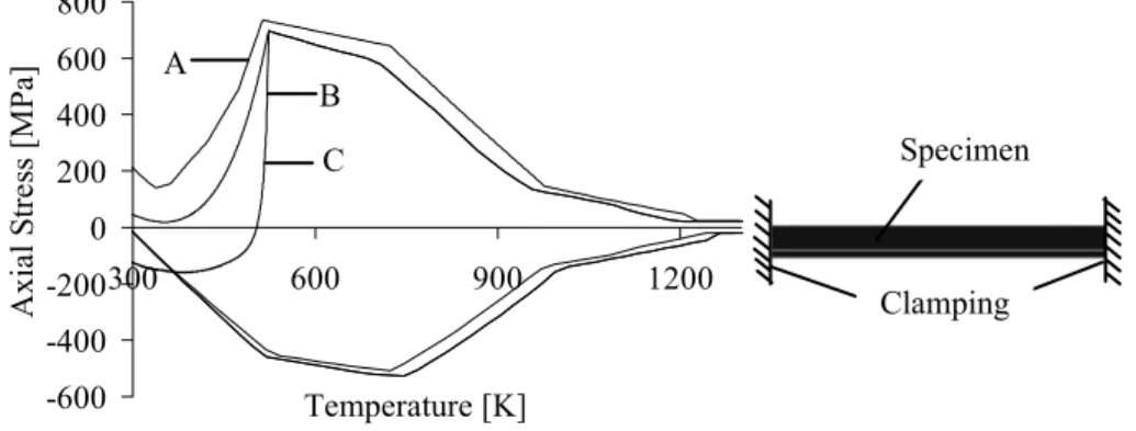
(22) Henrik Alberg – Material Modelling for Simulation of Heat Treatment model, described in Section 3.2, has been used for all sequences in the heat treatment simulation. However, observe to simulate of creep during the holding sequence the elastic domain was removed and material parameters were changed. The change of parameters during creep is due to the different times scale for the creep process. A comparison using different material models in welding and stress relief heat treatment simulations is presented in Paper C. In Paper C the matter in the simulation is a martensitic stainless steel. The microstructural evolution in steel has made it necessary model the effect due phase transformations. In the modelling of phase changes, two features have to be considered. Firstly, models for the microstructure evolution has to be stated. Secondly, the knowledge of how and if material properties are affected by phase changes has to be obtained. In the presentation of phase transformation modelling that will follow, steel is treated. However, the theory can be extended to other materials. The microstructure evolution for a diffusional transformation, for example transformation from ferrite/pearlite to austenite, Equation 11, can be used. Equation 11 is based on the theory by Kirkaldy et al. [21] and is proposed by Oddy et al. [22] for low carbon steel. n −1.   z eu   n  z& a = n ⋅  ln     z eu − z a   z& a is the austenite transformation rate, za the volume.  z − za  ⋅  eu (11)  τ   fraction of austenite, and zeu the phase. equilibrium. The parameterτ is a function of temperature and τ0, τe, and n are material constants. The calculation of the amount of martensite can be based on Koistinen-Marburger´s equation, Equation 12 where b’ is a material constant.. z m = 1 − e −b ⋅(M s −T ) (12) Transformation does not only lead to change in the mechanical properties but also in the transformation strain εtr. For sufficiently high stresses, plasticity is induced in the weaker phase; this is often referred to as the Greenwood-Johnson mechanism, Leblond [23]. In Paper C the orientation, behaviour of the created martensite due to an external load is not included; the same assumption is also used by Vincent et al. [24]. The mechanism often referred to as the Magee mechanism can effect the overall shape of the body. In this case the transformation is divided in a volumetric transformation strain εtra and a deviatoric transformation strain εtp, the last term is often referred to as the transformation induced plasticity strain (TRIP). The expression for the TRIP can be found in Paper C. ′. To account for the phase transformation in a simulation some material properties are changed while some are assumed independent of material phase. In the simulations performed in Paper C, it is assumed that Young’s modulus, Poisson’s ratio, and the thermal properties not are affected by the phase transformation, Börjesson et al. [25]. While yield limit (Figure 10), the evolution of the hardening and the parameters in the viscoplastic flow equation, Equation 9a, are assumed to be affected by the phase changes. Different phases usually have different densities, this is included in the simulation by changes in the thermal dilatation when different phases developing. To calculate the current value of the properties affected by the phase transformation, for example change in yield limit a rule of mixture can be used. In Paper C a linear rule of mixture is used, Equation 13 and 14, while Leblond [23] uses a nonlinear rule of mixture. Y = z fp Y fp + z a Ya + z m Ym (13). 14.

(23) Henrik Alberg – Material Modelling for Simulation of Heat Treatment z fp + z a + z m = 1 (14) zfp is the volume fraction of the mixture of ferrite/pearlite, za is the volume fraction of austenite, and zm is the volume fraction of martensite. Yfp is the material property for the mixture of ferrite/pearlite, Ya is the material property for austenite, and Ym is the material property for martensite. All data for the mechanical properties are presented in Paper C.. To illustrate how the different material behaviour affect the stress, a simulation of a Satoh test has been performed, Figure 11. In a Satoh test is a specimen clamed between two rigid walls. The specimen is then heated and the stress is measured. This test was originally made to simulate material behaviour during welding.. Axial Stress [MPa]. 800 600 400 200. A. B Specimen Specimen. C. 0 -200 300. 600. 900. 1200. Clamping Clamping. -400 -600. Temperature [K]. Figure 11. Satoh test. Curve A – no microstructural behaviour accounted for. Curve B – microstructural changes as described above calculation. Curve C– microstructural changes as described above including TRIP. The microstructure evolution in steel has been under a lot of research during the last century. Because of the commercial interest in steel, there exists several software that can calculate the microstructure evolution given the chemical composition, Lindgren [26]. The effects from tempering have not been studied in this thesis. However, simulations have been for example carried out by Ju et al. [9]. Simulation of ageing is not as common as the simulation of quenching. The metallurgists usually give the thermal cycle for this heat treatment process. They have good knowledge how the phases in the material evolve, and how to avoid unwanted effects like grain growth. However, interesting field for ageing simulations is in problems with strain-age cracking and in local heat treatment of repair welding. No simulations of this type have been performed by the author.. 4.2. Modelling of Thermal Boundary Conditions. An important subject in heat treatment simulation is how well the boundary conditions in the model correlate with the actual process. The mechanical boundary condition is often simple since the component is placed on a grid or a plate during the heat treatment. However, the thermal boundary conditions are more complex and will be examined in the subsequent sections for the heating and cooling sequences. The holding sequence does not usually give any problems regarding the thermal boundary condition.. 15.

(24) Henrik Alberg – Material Modelling for Simulation of Heat Treatment. 4.2.1. Heating Sequence. The heating during the heating sequence is generated in the furnace by radiators, c.f. Section 2.2.3, and is transferred to the component by thermal radiation. This kind of heat transfer simulations are presented in Papers A and C. The temperature of the furnace wall following a given profile and is controlled by during the heat treatment. The given profile may have different heating rates for different temperature intervals and may have a plateau, Figure 8, to get a more even distribution of temperatures in a geometrically difficult component. The radiative heat transfer has aspects that are not trivial in numerical simulation. The FE-software used in the simulation in this thesis is MSC.MARC. MARC calculates the radiative heat transfer using Equation 15a, where q is the heat flux, σSB is Stefan-Boltzmann’s constant, F is the viewfactor, T1 and T2 is the temperature of the surfaces having the heat transfer, respectively, Figure 12. cos φ1 cos φ 2 1 q = σ SB F T14 − T24 F= dA2 dA1 (15a,b) A1 πr 2. (. ). ∫∫. A1 A2. The viewfactors present how much an element sees another element, Figure 12. The viewfactor defined by a fourth order integral, Equation 15b. The calculations of the viewfactors are generally nontrivial and become even more complex including shadowing effects, MARC-manual [27]. The variables in Equations 15a and b are defined in Figure 12. In MARC the viewfactor integrals are determined using the Monte Carlo method. φ2 A1. r. A2 T2. φ1. T1. Figure 12. Viewfactor Definition In a simulation, where convection not can be neglected during the heating sequence a flow simulation like the one discussed in the next section may be performed.. 4.2.2. Cooling Sequence. During the cooling sequence most of the heat transfer is carried out by convective heat transfer, Section 2.2.3. The amount of energy transferred from the component to the surroundings is mainly dependent on two parameters, the temperature difference between the component surface and the surrounding and the heat transfer coefficient, Equation 16. The heat transfer coefficient can depend on the condition in the boundary layer, that are influenced by surface geometry, the nature of the fluid motion, and an assortment of fluid thermodynamic and transport properties, Incropera et al [28].. 16.

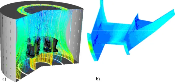
(25) Henrik Alberg – Material Modelling for Simulation of Heat Treatment. (. q& surface = h ⋅ Tsurface − T∞. ). (16). In Paper A, a method is developed and an analysis is carried out to obtain an approximate distribution of the surface heat transfer coefficient when an aerospace component is cooled in a heat treatment furnace. The simulation is made in two stages. The fluid flow is solved first and the computational fluid dynamics code FLUENT2 was used. The model used is shown in Figure 13a. The solution for the heat transfer coefficient was processed to give the boundary condition using Equation 16 in the thermo-mechanical finite element analysis. The coupling was accomplished by: I. Solving the fluid flow problem and computing the connective heat transfer coefficient h between the gas and the component using Equation 16. II. Applying the heat transfer coefficient from step I to the FE-model, as a boundary condition. III. Solving the thermo-mechanical problem In the fluid flow simulation the standard k-ε turbulence model, described in the FLUENT manual [29], and resolved boundary layer, describe in Paper A, was used for all cases. The fluid flow analysis was made with a 3D-model with the boundary conditions given in Paper A. The inclusion of the computed convective heat transfer coefficient into the finite element model was done using user-subroutines. The coupling was one-way; i.e. the deformation predicted by the FE-calculation is assumed not to affect the flow calculation, as the deformations involved are small, about 3 mm. Figure 13a and b show a velocity profile and heat transfer coefficient from a simulation in FLUENT.. a). b). Figure 13. a) Gas flow in a heat treatment furnace during the cooling sequence. B) Surface heat transfer coefficient with the gas flow from Figure 13a) during cooling sequence Figure 14 shows the heat flux experienced by a given point on the component during cooling. The peaks are associated with changes in the direction of flow and are due to turbulence. However, 2. FLUENT – a commercial software to solve fluid and thermal-fluid mechanics problems 17.

(26) Henrik Alberg – Material Modelling for Simulation of Heat Treatment. 45000 40000 35000 30000 25000 20000 15000 10000 5000 0. 1100. Temperature. 1000 900. q&wall. 800 700 600 500 400. Temperature [K]. q&wall [W/m2]. these disturbances only affect a short period, compared with the steady state phase. The change in flow direction is modelled by taking the result of heat transfer coefficient or a converged stationary solution in each flow direction. Note that the heat flux in Figure 14 reduces over time because of the decreasing temperature of the component surface.. 300. 0. 10. 20. 30. 40. 50. 60. 70. 80. Time [s]. Figure 14. Calculated heat flux, q& wall on the component from the FLUENT-model at a single point on the component, from Paper A. Similar simulations have been performed by Lind et al. [30]. They also used fluid mechanics simulations to obtain an approximate distribution of the surface heat transfer coefficient when quenching a steel cylinder in a gas cooled furnace.. 18.

(27) Henrik Alberg – Material Modelling for Simulation of Heat Treatment. 5. Summary of Appended Papers. In Paper A, combined welding and heat treatment simulation is performed on an aerospace component. The geometrical tolerances are important to control in the manufacturing in order to maintain the quality with reduced lead time and cost. Simulation can be a tool to obtain information about dimension, shape, and residual stresses after each process. Paper A presents a simulation method for combined welding and stress relief heat treatment analysis and the use of computational fluid dynamics to estimate the heat transfer coefficient on the component’s surface. Paper B presents a combined approach where the same numerical implementation of a constitutive model to be used in the finite element code is used for material parameter identification. Different material models, numerical algorithms, and methods for parameter identifications are discussed to set the general context and an application of the toolbox for Greek Ascoloy is described. A parameter fitting using a viscoplastic model with nonlinear isotropic hardening is performed. The method of using fluid flow calculation as a boundary condition in a thermo-mechanical simulation and the knowledge about the welding and heat treatment simulation obtained in Paper A. And the tool developed and material parameters obtained in Paper B are applied in Paper C. In Paper C a comparison to see how different material behaviour affects the response from combined welding and heat treatment on an aerospace component are made. The simulation is made on the same component as in Paper A. The material models include different effects like rate-independent and viscoplastic models including microstructure calculation and transformation induced plasticity. Different creep models and different way to apply them has also been investigated.. 19.

(28) Henrik Alberg – Material Modelling for Simulation of Heat Treatment. 6. Discussions and Future Work. The aim of the current work is to develop an efficient and reliable model for simulation of heat treatment. Using an axisymmetric model for simulation of welding and heat treatment has shown to give acceptable simulation time, even when using a viscoplastic model, including phase transformations and TRIP. The stress relief heat treatment process in a gas cooled vacuum furnace has been simulated using radiation boundary conditions for the heating sequence and convective boundary condition during the cooling. Gas flow simulation has shown a useful tool when predicting the boundary condition during the cooling stage. Furthermore, it has been shown that this boundary condition is strongly dependent on the position of the component in the furnace. Moreover, stationary flow in each direction in the furnace can be assumed even if the flow direction reverted every 10 seconds. Furthermore, it has been found that the cooling stage of the heat treatment process does not give rise to any additional plastic strains. Different material models for welding and heat treatment simulations have been compared. The simulation reviled that using different material models gave differences in final shape and residual stresses after welding and heat treatment. It has been found that the heat treatment reduced residual stresses and the shrinkage caused by the welding process. Furthermore, it has been found that the choices of creep model have only minor importance on the final shape and the residual stresses. When a constitutive model with several material parameters is to be used in a simulation, it may be difficult to find the material parameters. Due to the limitation in cost, time and the difficulty to design test, such that each material parameter can be studied independently when material parameters are to be decided, a parameter fitting tool has shown to be of importance. The lack of experimental data for the component makes it impossible to come to any conclusion regarding the choice of material model can be made from reliability and accuracy point of view. The questions regarding accuracy and reliability of the models are still not completely answered due to the lack of experimental data for the component; it will therefore be important to acquire such data. Further work will also evaluate the use of shell elements in heat treatment simulations. The use of shell elements in will decrease the simulation time. The need for different accuracy in different part of the product development has to be further investigated to be able to make acceptable simplifications.. 20.

(29) Henrik Alberg – Material Modelling for Simulation of Heat Treatment. References [1] [2] [3] [4] [5] [6]. [7] [8] [9]. [10] [11] [12] [13] [14] [15] [16] [17] [18] [19]. Hibbit, L-E and Marcal, P.V. A numerical thermo-mechanical model for the welding and subsequent loading of a fabricated structure, Computers and Structures (1973) 1145-1174. Ueda, Y. and Yamakawa, T. Analysis of thermal elastic-plastic stress and stress during welding by finite element method, Trans. Japan Welding Society 2 (1971) 90-100. Burnett, J.A. and Pedovan, J. Residual stress field in heat treated case-hardened cylinders. Journal of Thermal Stresses 2 (1979), 251-263. Sjöström, S. The calculation of quench stresses in steel, Ph.D. theses no 84, University of Linköping, Sweden, 1982. Rammerstorfer, F.G., Fischer, D.F., Mitter, W., Bathe, K.J. and Snyder, M.D. On thermoelastic-plastic analysis of heat-treatment processes including creep and phase changes. Computer and Structures 13 (1981) 771-779. Donzella, G., Granzotto, S., Amici, G., Ghidini, A. and Bertelli, R. Microstructure and Residual Stress Analysis of a Rim Chilled Solid Wheel for Rail Transportation System, Computer Methods and Experimental Measurements for Surface Treatment Effects II, (1995), 293-300. Thuvander, A. Calculation of distortion of tool steel dies during hardening, in: Proc. 2nd International Conference on Quenching and the Control of Distortion, (USA, Cleveland/Ohio, 1996), 297-304. Tajima, M. Prediction of Hardness Variations in Quenching of Carbon Steel, in: Proc. 2nd International Conference on Quenching and the Control of Distortion, (USA, Cleveland/Ohio, 1996), 291-296. Ju, D.Y., Sahashi, M.M., Omori, T. and Inoue, T. Residual Stresses and Distortion of a Ring in Quenching-Tempering Process Based on Metallo-Termo-Mechanics, in: Proc. 2nd International Conference on Quenching and the Control of Distortion, (USA, Cleveland/Ohio, 1996), 249-257. Josefson, B.L. Residual stresses and their redistribution during annealing of a girth-butt welded thin walled pipe. Journal of Pressure Vessel Technology 104 (1982) 245-250. Wang, J., Lu, H. and Murakawa, H. Mechanical Behaviour in Local Post Weld Heat Treatment, JWRI 27 (1998) 83-88. Shackelford, J.F. Introduction to material science, SI Edition - Fourth edition. (Prentice Hall Europe, Upper Saddle River, 1998), ISBN 0-13-807125-X. Callister, W.D. Materials science and engineering, An introduction Third Edition. (John Wiley & Sons, Inc, New York, 1994), ISBN 0-471-30568-5. Stouffer, D.C. and Dame, L.T. Inelastic Deformations of Metals - Models, mechanical properties and metallurgy (John Wiley & Sons, New York, 1996). Davis, J. R. (ed.) et al., ASM Handbook – Vol4: Heat treating. 1991, ISBN 0-87170-379-3. Lemaitre, J. and Chaboche, J.-L. Mechanics of solid materials (Cambridge University Press, Cambridge, 1990). Miller, A.K. The MATMOD equations, in Unified Constitutive Equations for Creep and Plasticity, A.K. Miller, Editor (Elsevier Applied Science Publishers Ltd., Amsterdam, 1987). Belytschko, T. Liu, W.K. and Moran, B. Nonlinear Finite Elements for Continua and Structures (John Wiley & Sons, Chichester, 2000). Simo, J.C. and Hughes, T.J.R. Computational Inelasticity (Springer-Verlag, New York, 1997).. 21.

(30) Henrik Alberg – Material Modelling for Simulation of Heat Treatment [20] [21] [22] [23] [24] [25] [26] [27] [28] [29] [30]. 22. Chaboche, J.-L. Viscoplastic Constitutive Equation for the Description of Cyclic and Anisotropic Behaviour of Metals: 17th Polish Conference on Mechanics of Solids, Szczyrk Bul de l’Acad Poloaise des Science, Série Sc et Techn, Vol 25 (1975) pp. 33Kirkaldy, J.S and Venugopalan, D. Prediction of Micriostructure and Hardenabillity in Low alloy Steels, Proc: Int. Conf. On Phase Transformation in Ferrous Alloys, (1983), 125-148. Oddy, A.S., McDill, J.M.J. and Karlsson, L. Microstructural Predictions Including Arbitrary Thermal Histories, Reaustenization and Carbon Segregation Effects, Can Metall. Q., No 3, p 275-283, 1996. Leblond, J.B Mathematical Modelling of transformation plasticity in steels (Part I and II), Int. Journal of Plasticity 5 (1989) 551. Vincent, Y., Jullien, J.F., and Gilles, P. Thermo-Mechanical Consequences of Phase Transformation in the Heat Affected Zone using a Cyclic Uniaxial Test, Int. Journal of Solids and Structures, to be published. Börjesson, L. and Lindgren, L-E. Simulation of multipass welding with simultaneous computation of material properties, Journal of engineering materials and technology, 123 (2001) 106-110. Lindgren, L-E. Finite element modelling of welding. Part 2: Improved material modelling, Journal of Thermal Stresses 24 (2001) 195-231. MARC Reference Manual Incropera, F. P. and DeWitt, D.P. Fundamentals of heat and mass transfer, Forth Edition, (John Wiley & Sons , New York, 1996). Fluent Reference Manual Lind, M., Lior, N., Alavyoon, F. and Bark, F. Flow effects and modelling in gas-cooled quenching, in: Proc. of the 11th International Heat Transfer Conference, Vol. 3, (Korea, Kyongju, 1998), 171-176.

(31)

No results found