https://doi.org/10.1007/s00382-019-04906-x
European marginal seas in a regional atmosphere–ocean coupled
model and their impact on Vb‑cyclones and associated precipitation
Naveed Akhtar1,6 · Amelie Krug1 · Jennifer Brauch2 · Thomas Arsouze3,4 · Christian Dieterich5 · Bodo Ahrens1
Received: 30 July 2018 / Accepted: 18 July 2019 / Published online: 1 August 2019 © The Author(s) 2019
Abstract
Vb-cyclones are extratropical cyclones propagating from the Western Mediterranean Sea and traveling across the Eastern Alps into the Baltic region. With these cyclones, extreme precipitation over Central Europe potentially triggers significant flood events. Understanding the prediction ability of Vb-cyclones would lower risks from adverse impacts. This study ana-lyzes the robustness of an atmosphere–ocean regional coupled model, including interactive models for the Mediterranean Sea (MED) and North and Baltic Seas (NORDIC) in reproducing observed Vb-cyclone characteristics. We use the regional climate model (RCM) COSMO-CLM (CCLM) in stand-alone and coupled with the ocean model NEMO configurations for the EURO-CORDEX domain from 1979 to 2014, driven by the ERA-Interim reanalysis. Sea surface temperature (SST) is evaluated to demonstrate the stability and reliability of the coupled configurations. Compared to observations, simulated SSTs show biases (~ 1 °C), especially during winter and summer. Generally, all model configurations are able to replicate Vb-cyclones, their trajectories, and associated precipitation fields. Cyclone trajectories are comparably well simulated with the coupled models, as with the stand-alone simulation which is driven by the reanalysis SST in the MED and NORDIC seas. The cyclone intensity shows large deviations from reanalysis reference in the simulations with the interactive MED Sea, and smallest with CCLM. Precipitation characteristics are similarly simulated in the coupled and stand-alone (with reanalysis SST) simulations. The results suggest that our coupled RCM is useful for studying the impacts of highly resolved and interactively simulated SSTs on European extreme events and regional climate, a crucial prerequisite for understanding future climate conditions.
Keywords Mediterranean Sea · North and Baltic Seas · Ocean coupling · Vb-cyclones
1 Introduction
The Mediterranean region is one of the world’s primary cyclogenetic regions (Petterssen 1956; Hoskins and Hodges 2002; Wernli and Schwierz 2006). Complex air-sea inter-actions and orographic features play a predominant role in determining the Mediterranean climate. For example, high evaporation over the Mediterranean Sea favors frequent cyclonic activities in the region (Alpert et al. 1995). One specific type of cyclone that develops over the Western Mediterranean Sea, typically over the Gulf of Genoa, and travels across the Eastern European Alps toward the Baltic region is the Vb-cyclone (Van Bebber 1891; Messmer et al. 2015). Persistent strong cut-off lows drive synoptic scale atmospheric circulation, including the Vb-pathway, and are responsible for extreme weather conditions (Stucki et al. 2013; Ulbrich et al. 2003a, b). A typical Vb-type weather condition occurs when a high-pressure system is located
Electronic supplementary material The online version of this
article (https ://doi.org/10.1007/s0038 2-019-04906 -x) contains supplementary material, which is available to authorized users. * Naveed Akhtar
naveed.akhtar@hzg.de
1 Institute for Atmospheric and Environmental Sciences,
Goethe University, Frankfurt, Germany
2 Deutscher Wetterdienst, Offenbach am Main, Germany 3 ENSTA ParisTech, Université Paris-Saclay, Paris, France 4 Laboratoire de Meteorologie Dynamique, Ecole
Polytechnique, Palaiseau, France
5 Swedish Meteorological and Hydrological Institute,
Norrköping, Sweden
6 Present Address: Institute of Coastal Research,
over the Baltic region and, at the same time, an intense low-pressure system moves from the Western Mediterranean Sea toward Central or Eastern Europe. During such events, significant moisture is transported towards the northern side of the Alps and into Central Europe due to the counterclock-wise rotation of the cyclone. Such a condition can last for several days and often yields large-scale intense precipita-tion events and floods in Central Europe (Mudelsee et al. 2004; Nied et al. 2014). Hofstätter et al. (2018) reported that during summer almost every second Vb-cyclone is related to heavy precipitation over the Czech Republic and Austria. The authors also found that the precipitation intensity asso-ciated with Vb-cyclones is high in summer due to high air temperatures. In addition, Nissen et al. (2013) showed that flooding associated with Vb-cyclones is mainly a summer phenomenon. Examples of extreme Vb flood events include those in Switzerland in September 1993 (Stucki et al. 2013), the Czech Republic and Austria in July 1997 (Ulbrich et al. 2003b; Cyberski et al. 2006; Godina et al. 2006; Ho-Hage-mann 2015), Central Europe in August 2002 (Ulbrich et al. 2003a; Grazzini and van der Grijn 2002), the Alpine region in August 2005 (Beniston 2006), and in Central Europe in May–June 2013 (Grams et al. 2014; Kelemen et al. 2016) and May 2014 (Stadtherr et al. 2016). Such extreme events often led to substantial economic and personal losses (Graefe and Hegg 2004; MeteoSchweiz 2006; Mitzschke 2013; Held et al. 2013).
The Mediterranean region is often referred as a climate change “hotspot” for global warming (Giorgi 2006). Strong warming of the Mediterranean Sea surface temperature (SST) was already being observed already by the end of the 20th century (Rixen et al. 2005). By the end of the 21st century, more than 2 K additional warming is predicted compared to 1980–1999 (IPCC 2007, 2013). These ther-modynamic changes may significantly change the air-sea interaction, which can influence the occurrence and inten-sity of Mediterranean cyclones. Although mean precipitation is expected to decrease in the long-term (Christensen and Christensen 2007), an increase in evaporation and moisture transport can potentially impact short-term extreme precipi-tation events over Central Europe (e.g., Gimeno et al. 2010; Volosciuk et al. 2016; Messmer et al. 2017). A decrease in frequency and an increase in intensity of Vb-cyclones is projected under future climate change conditions (Muskulus and Jacob 2005; Nissen et al. 2013).
The dynamics of synoptic-scale atmospheric circula-tion and the contribucircula-tion of moisture flux from differ-ent sources influence the precipitation amount associated with Vb-cyclones (Messmer et al. 2015). The precipita-tion is potentially most intense if the cut-off low is located over the northern or eastern parts of the Alps (Awan and
Formayer 2016). Gimeno et al. (2010) and Volosciuk et al. (2016) found that intense precipitation events over Central Europe are directly linked to the thermodynamic conditions in the Mediterranean area. However, most Vb studies have focused on individual cases, and thus general conclusions have to be made with care. For example, the August 2002 event is one of the most frequently analyzed cases (Ulbrich et al. 2003a, b; Grazzini and van der Grijn 2002; Stohl and James 2004; James et al. 2004; Kaspar and Müller 2008). In addition to evaporation over the Mediterranean Sea, inland evaporation was a major source of moisture for the August 2002 Vb-event (Ulbrich et al. 2003a; Sodemann et al. 2009). Sodemann et al. (2009) further proposed that the Atlantic and long-range advection should not be ignored. The latter is supported by Winschall et al. (2014), who investigated various extreme precipitation events over Central Europe and recognized that the North Atlantic, in addition to the Mediterranean Sea and inland evaporation, is an important moisture source. Similar conclusions were also drawn by James et al. (2004) and Stohl and James (2004) using a backward tracking method and particle dispersion model, respectively, in analyzing the August 2002 case. In contrast, Gangoiti et al. (2011) concluded that the Mediterranean Sea was the main moisture source for the August 2002 Vb-event. In a recent model-based study, Messmer et al. (2017) found a non-linear relationship between Mediterranean SST and precipitation intensity. An increase of 5 K in Mediterranean SST increases the precipitation amount by 24%, whereas a 5 K reduction induces a decrease of only 9% in precipitation intensity over Central Europe during Vb-events. However, no significant differences in the precipitation intensity were found between + 1 and + 3 K.
Most Vb-cyclone studies investigated reanalysis datasets or uncoupled regional or global atmospheric model simula-tions, which exhibit considerable uncertainty (− 7 ± 21 W/ m2) in the Mediterranean Sea surface heat fluxes
(Sanchez-Gomez et al. 2011). These uncertainties can strongly affect the intensity and tracks of Mediterranean cyclones. Cur-rently, state-of-the-art regional climate models (RCMs) achieve horizontal resolutions finer than 50 km, which pro-vides a more realistic representation of local features (Her-rmann and Somot 2008). However, RCMs often use coarse-resolution SST from coupled global model simulations or reanalysis (e.g., ERA-Interim and NCEP/NCAR) datasets as lower boundary conditions (Christensen and Christensen 2007). These datasets do not represent the European mar-ginal seas (Mediterranean, North and Baltic Seas) well, although SST variations in these marginal seas are essential to regional climate at different temporal and spatial scales (Somot et al. 2008; Li 2006; Akhtar et al. 2018).
Recently, atmosphere–ocean regional climate mod-els (AORCMs) became available and they represent an opportunity to study the impact of increased resolution and air–sea coupling on extreme events, such as Vb-cyclones. Studies show that air–sea coupling over mar-ginal seas affects simulated temperature and precipitation both over the coupling domain, and over land (e.g., Somot et al. 2008; Pham et al. 2014; Ho-Hagemann 2015). Fur-thermore, SSTs simulated with high-resolution (less than 10 km grid distance) ocean models can have a strong and beneficial effect on cyclogenesis and precipitation (Sanna et al. 2013). Akhtar et al. (2014) showed that a high-resolution AORCM improves trajectories and the inten-sity of simulated Mediterranean hurricanes (medicanes) compared to RCM due to better resolved mesoscale pro-cesses and turbulent fluxes. An improved representation of simulated fluxes, including momentum fluxes, using an AORCM instead of an RCM was also shown in Akhtar et al. (2018). There is general agreement that high-resolu-tion AORCMs are a prerequisite for resolving small-scale features of the Mediterranean (e.g., Somot et al. 2008; Herrmann et al. 2011; Ruti et al. 2016) and North and Baltic Seas (e.g., Pham et al. 2014; Ho-Hagemann 2015).
The value of using AORCMs was highlighted by Ho-Hagemann (2015), who used an AORCM with a coupled North and Baltic Seas model to investigate the July 1997 Oder flooding event, which was associated with a sequence of two Vb-cyclones (“Xolska” and “Zoe”). For the second Vb, they identified a large-scale convergence of moisture from the Mediterranean Sea, together with moisture com-ing from the North Atlantic Ocean via the North Sea and inland evaporation, as responsible for heavy rainfall and floods in Central Europe. Their analysis explicitly showed the added value of coupled North and Baltic Seas mod-els for simulating the event. The impact of air-sea inter-actions and feedbacks over European marginal seas, the Mediterranean Sea, and the North and Baltic Seas on the characteristics of Vb-cyclones have not yet been investi-gated using an AORCM. The present work evaluates SST that is simulated using newly developed AORCMs and addresses the impact of atmosphere–ocean coupling (1) over the Mediterranean Sea, (2) over the North and Baltic Seas, and (3) over the marginal seas in a combined system on trajectories and precipitation characteristics of selected Vb-cyclones in the ERA-Interim period.
This paper is structured as follows. Section 2 describes the details of the models, experimental design, datasets, and analysis methods. The results and discussion are pro-vided in Sect. 3. Finally, the main conclusions and future research perspectives are presented in Sect. 4.
2 Modeling system and experimental
configuration
In this study, we used the COSMO-CLM (CCLM) RCM in combination with regional ocean models NEMO-MED12 for the Mediterranean Sea and NEMO-NORDIC for the North and Baltic Seas to generate three AORCMs for analyses.
2.1 CCLM
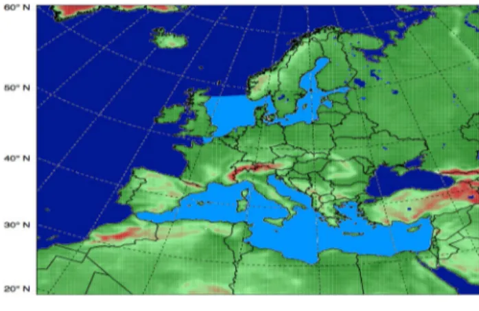
The atmospheric model CCLM v5.7 is a non-hydrostatic RCM based on primitive equations (Rockel et al. 2008). The model configuration follows the EURO-CORDEX extent (Fig. 1) (Giorgi et al. 2006; Van Pham et al. 2014) with an atmospheric grid resolution of 0.22° (~ 25 km, 232 × 226 grid points and 40 σ levels). In our configura-tion, CCLM uses a numerical time step of 150 s with a third order Runge–Kutta numerical integration scheme aerosol optical depth data following Tegen et al. (1997). Further-more, CCLM uses a one-dimensional prognostic turbulent kinetic energy scheme for vertical turbulent diffusion param-eterization and a delta-two–stream radiation scheme (Ritter and Geleyn 1992). To better represent sea ice in the North and Baltic Seas, a sub-grid scale sea ice mask was imple-mented in the CCLM coupled configuration over the region to account for partially sea ice covered grid boxes. In the coupled setup, the CCLM model receives the sea ice mask from NEMO-NORDIC and calculates the weighted average of the albedo in a grid cell based on the fraction of ice and open water (Pham et al. 2014). The initial and lateral bound-ary conditions for CCLM were taken from the European Centre for Medium-Range Weather Forecast’s (ECMWF) ERA-Interim reanalysis provided every 6 h with 0.75° grid resolution for 1979–2014 (Dee et al. 2011). However, in the coupled configurations, the SSTs and ice fraction (only for
Fig. 1 Atmospheric model domain, sky blue color indicates the cou-pling regions for the Mediterranean Sea and North and Baltic Seas
the North and Baltic Seas) in the coupling regions (Fig. 1) are calculated using the following regional ocean models.
2.2 NEMO‑MED12
NEMO-MED12 is a regional implementation of the ocean general circulation model NEMO v3.6 (Madec and NEMO Team 2008) for the Mediterranean Sea (Beuvier et al. 2012; Lebeaupin et al. 2011, 2012; Akhtar et al. 2018). The NEMO-MED12 grid covers the entire Mediterranean Sea plus a small part of the Atlantic Ocean west of Gibraltar which acts as a buffer zone for open boundary conditions (Beuvier et al. 2012). However, the coupling is only per-formed over the Mediterranean Sea (Fig. 1). It has the stand-ard irregular ORCA grid with 1/12° resolution (~ 6.5–8.0 km in latitude and ~ 5.5–7.5 km in longitude; 567 × 264 grid points). In the vertical, 75 unevenly z-levels are used with a layer thickness of 1 m at the surface, increasing to 135 m at the bottom. It is an eddy-resolving regional ocean model, as the Rossby radius for deformation over the Mediterranean Sea is on the order of 15 km (Lebeaupin et al. 2011). In our configuration, the numerical time step of the model is 720 s. The initial conditions for three-dimensional poten-tial temperature and salinity are provided by the MEDAT-LAS-II (Rixen 2012) monthly mean seasonal climatology (1945–2002) in the Mediterranean Sea. A 30-year coupled spin-up simulation driven by randomly resampled ERA-Interim data (1979–1990) balanced the initial state. Water exchange with the Atlantic Ocean is relaxed to the Levitus et al. (2005) climatology prescribed in the buffer zone. The Black Sea and runoff water input were prescribed from the climatological average of interannual data from Ludwig et al. (2009). Further details are provided in Beuvier et al. (2012), Lebeaupin et al. (2011), and Akhtar et al. (2018).
2.3 NEMO‑NORDIC
NEMO-NORDIC is a regional implementation of the NEMO v3.3 for the North and Baltic Seas (e.g., Hodoir et al. 2013; Dieterich et al. 2013; Van Pham et al. 2014). The NEMO-NORDIC grid covers the entire Baltic and North Seas, with two open boundaries in the Atlantic Ocean. The northern zonal boundary is the cross-section between the Hebrides and Norway and the southern meridional boundary lies in the English Channel (Fig. 1). It has a resolution of 2 nautical minutes (~ 3.7 km; 619 × 523 grid points) and 56 stretched vertical levels with a thickness of 3 m at the surface and 22 m at the bottom of the Norwegian Sea. Such a high horizontal resolution allows the mesoscale variability to be marginally resolved in the North and Baltic Seas (Meier and Kauker 2003), because the average Rossby radius of defor-mation over the Baltic Sea is on the order of 7 km (Osiński et al. 2010). NEMO-NORDIC uses the NEMO sea ice model
LIM3, which includes the dynamics and thermodynamic processes of sea ice (Vancoppenolle et al. 2009). NEMO-NORDIC employs a numerical time step of 180 s and free surface scheme to include tidal forcing in the dynamics. The tidal potential is prescribed at the open boundaries in the North Sea from the global tidal model of Egbert and Ero-feeva (2002) and Egbert et al. (2010). The initial conditions for three-dimensional potential temperature and salinity are provided by Janssen et al. (1999) and the lateral boundary conditions in the North Sea are prescribed from ORAS4 reanalysis data (Balmaseda et al. 2013). Freshwater inflow of the rivers is provided from daily time series of the E-HYPE model output (Lindström et al. 2010).
2.4 Coupler and coupling fields
The coupling of the atmospheric (CCLM) and ocean models (NEMO-MED12 and NEMO-NORDIC) is achieved using the OASIS3-MCT coupler (Craig et al. 2017). The OASIS3-MCT coupler synchronizes the models and interpolates the coupling fields from one model grid to another. In the cou-pled setup, the ocean model sends SST to CCLM through OASIS3-MCT and in turn receives solar energy, non-solar heat, momentum, and freshwater fluxes. In addition, NEMO-NORDIC sends the sea ice fraction to CCLM and receives sea level pressure. The coupling fields are exchanged every 3 h. A more detailed description of the coupling strategy and its implementation can be found in Will et al. (2017).
2.5 Experiment and analyses methods
Hereafter, “CCLM” refers to uncoupled CCLM simulations, “MED” refers to CCLM coupled with NEMO-MED12, “NORDIC” refers to CCLM coupled with NEMO-NOR-DIC, and “MED + NORDIC” refers to CCLM simulations simultaneously coupled with the two regional ocean mod-els NEMO-MED12 and NEMO-NORDIC. Four simulations (CCLM, MED, NORDIC, and MED + NORDIC) were per-formed for 1979–2014.
Firstly, the newly developed AORCM with one or two coupled European marginal seas was evaluated comparing mean simulated seasonal and annual SST over the coupling region with observations. Next, eight Vb-type events were selected from 1979 to 2014 (Table 1). These Vb-events trig-gered extreme precipitation over the northern slopes of the Alps and in Central Europe (e.g., Hofstätter and Chimani 2012; Messmer et al. 2017; Ho-Hagemann 2015). The first two Vb-events in July 1981 and August 1985 were relatively weak events in terms of precipitation intensity (Messmer et al. 2017). The later events were associated with extreme floods, as described in Sect. 1.
The cyclone trajectories in the reanalysis data and model simulations were detected with an objective method follow-ing Hofstätter and Chimani (2012), Hofstätter et al. (2016). As this tracking method works only for standard geographic grids, CCLM rotated horizontal wind and geopotential height fields were derotated and interpolated to a standard geographic grid. A discrete cosine filter (Denis et al. 2002) was applied to avoid spurious structures and false detections of cyclone centers due to local minima, especially at the edge of low-pressure systems. The low-pass filter removed structures smaller than 400 km, decreased smoothly up to 1000 km, and passed all large scales (Hofstätter and Chimani 2012). The cyclone centers were localized at each time step as closed local minima for a geopotential height of 700 hPa. To determine the corresponding cyclone center at the fol-lowing time step tn+1, a first guess was estimated. For the first guess, the predicted cyclone propagation vector, fol-lowing Hofstätter et al. (2016), Eq. (2), was applied. The horizontal wind at 700 hPa and 500 hPa was used for the first guess estimation. The detected cyclone center at tn+1 nearest to the position of the first guess was then chosen as the following track position. Based on this tracking method, it was not possible to detect continuous cyclone tracks for some events. In such cases, the corresponding following track some time steps later was considered.
To verify simulated cyclone precipitation against obser-vations, an object-based measure of the Structure, Ampli-tude, and Location (SAL) of the precipitation field in a pre-specified domain was calculated according to Wer-nli et al. (2008). A 30 × 30 model grid box, centered on the E-OBS’ precipitation maxima and threshold factor of 1/15 to identify objects was used to calculate SAL. An object defines a grid point of a local precipitation maxi-mum above threshold values, which includes neighboring grid points as long as the grid point values are larger than the threshold values (Wernli et al. 2008). The amplitude component A of SAL describes the normalized domain averaged field difference of the simulated and observed precipitation. Its values range from − 2 to + 2, with 0 indi-cating a perfect forecast and − 1/+ 1 indiindi-cating underesti-mation/overestimation of spatially averaged precipitation
by a factor of 3. The structure component S describes the volume of the normalized precipitation object, using its size and shape. It ranges from − 2 to + 2 with 0 indicat-ing area similarity of simulated and observed precipita-tion object. The third component, locaprecipita-tion L, computes the normalized distance between the center of mass of the simulated precipitation object and observed one. Addi-tionally, mean differences in daily precipitation values of simulations and observations were used as simple statisti-cal measures.
The following reference datasets were also incorporated into the analyses:
• NOAA Daily Optimum Interpolation SST (OISST), available from September 1981 to present on a 0.25° global grid every 6 h. It is based on observations from satellites, ships, and buoys (Reynolds et al. 2007). • ENSEMBLES observations (E-OBS) v15.0 precipitation
dataset, available from 1950 to present. Daily accumu-lated E-OBS precipitation values are used on the avail-able 0.22° rotated grid. It is based on station observations mainly over European land (Haylock et al. 2008). • ECMWF’s ERA-Interim reanalysis precipitation,
geo-potential height, and horizontal wind datasets, available from 1979 to present on a 0.75° global grid (Dee et al. 2011).
• NASA’s MERRA-2 reanalysis geopotential height and horizontal wind datasets, available from 1980 to present on a 0.5° × 0.625° grid (Gelaro et al. 2017).
3 Results and discussion
In this section, we analyze the ability of the uncoupled and coupled models in reproducing observed Vb-cyclone characteristics. Results from the newly developed regional atmospheric model coupled with two marginal seas are pre-sented for the first time; therefore, first, briefly evaluate the simulated SSTs for 1982–2014, which are distinct in coupled and uncoupled simulations.
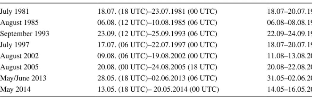
Table 1 Selected Vb-cyclone events
The second and third columns show the length of cyclone tracks in days presented in Fig. 4 and period with most extreme precipitation, respectively
July 1981 18.07. (18 UTC)–23.07.1981 (00 UTC) 18.07–20.07.1981
August 1985 06.08. (12 UTC)–10.08.1985 (06 UTC) 06.08–08.08.1985
September 1993 23.09. (12 UTC)–25.09.1993 (06 UTC) 22.09–24.09.1993
July 1997 17.07. (06 UTC)–22.07.1997 (00 UTC) 18.07–20.07.1997
August 2002 09.08. (06 UTC)–19.08.2002 (00 UTC) 11.08–13.08.2002
August 2005 20.08. (00 UTC)–24.08.2005 (18 UTC) 20.08–22.08.2005
May/June 2013 28.05. (18 UTC)–02.06.2013 (06 UTC) 31.05–02.06.2013
3.1 SST
Simulated SST time series averaged over each of the cou-pling regions were compared against observed OISST. Fig-ure 2 shows that simulated SSTs in MED + NORDIC display very small differences compared to MED or NORDIC-only simulations. The differences between CCLM and observed OISST are small, as the ERA-Interim forcing’s SSTs are based on observational data. The MERRA-2 SSTs similarly assimilate observational data.
Mediterranean SSTs were warmer in the coupled simula-tions for 1979–1995 than OISST and colder after 2005. The coupled simulations underestimate the warming trend after about 2005. In the uncoupled CCLM simulation, the trend is also less than in OISST after 2005. This underestimation of the warming trend might be linked to the atmospheric forc-ing, as the ERA-Interim SST is also underestimated com-pared to OISST after about 2005. These changes are related to the use of large numbers of observations in ERA-Interim, especially after 2005, which modify the shortwave radiations in ERA-Interim and in CCLM through atmospheric forcing (Fig. SI-1). Initially warm SST in the coupled simulations which can be due to atmospheric forcing, also reduced the warming trend.
In contrast, the North and Baltic SSTs in the coupled simulations are colder (up to approximately 0.5 °C) than OISST throughout the simulation period. Gröger et al. 2015 described the cold bias in the coupled (they used the same ocean component for the North and Baltic Seas as in this study) and uncoupled simulations. They argue that the cold ERA40 SSTs contribute to the cold bias in the uncoupled simulations. For the coupled simulation they argue that the initially too cold SSTs are prevailing
because of positive feedback with the atmosphere. Firstly, atmospheric surface temperatures would become too cold and thus support SSTs that are too cold. Secondly, the atmospheric boundary layer would be more stable in case of cold SSTs, which would decrease wind speeds and reduce vertical mixing, potentially deepening the oceanic mixed layer and increasing the heat capacity and temperature of the oceanic mixed layer. All simulations reproduced the SST interannual variability quite well in comparison to MERRA-2 and OISST. Notably, warming trends are larger in the North and Baltic Seas (NORDIC:
Fig. 2 Annual mean SST (°C) time series averaged over a the Mediterranean Sea and b the North and Baltic Seas for the period 1979–2014
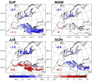
Fig. 3 Mean seasonal differences in SST (°C) between MED + NOR-DIC and OISST for 1982–2014. The colored numbers indicate mean differences (°C) in the Mediterranean Sea (red) and in North and Bal-tic Seas (blue)
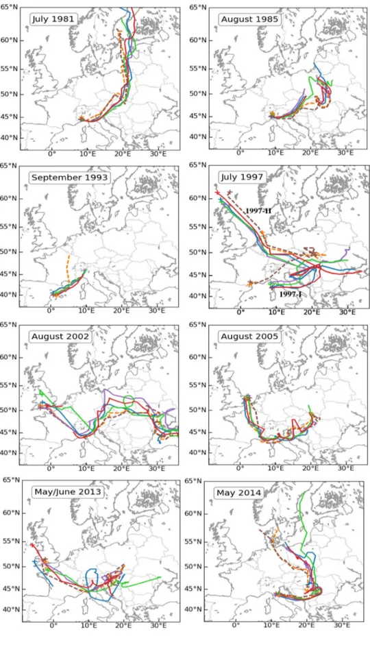
Fig. 4 Tracks of the eight selected Vb-cyclones from the CCLM (purple), MED (blue), NORDIC (green), MED + NORDIC (red), ERA-Interim (orange, dashed), and MERRA-2 (brown, dashed)
2.1 °C, ERA-Interim: 2.3 °C) than in the Mediterranean Sea (MED: 0.4 °C, ERA-Interim: 0.85 °C) for 1979–2014.
Figure 3 shows the mean seasonal differences between the coupled simulation MED + NORDIC and observa-tions for 1982–2014 (OISST is available from September 1981). The SST differences are most pronounced during summer (0.8 °C) and winter (− 1.1 °C) over the Medi-terranean Sea. Better agreement with the observations is found for the spring season. Locally, in the Levantine basin and the central Mediterranean Sea, these differences are up to ± 2.5 °C. During summer there is a prevailing warm bias in the south-east Mediterranean Sea and cold bias (up to − 0.5 °C) in the north-eastern and the Adri-atic basin. It corresponds to the prevailing anti-cyclonic oceanic structures along the south-eastern coasts and to the cyclonic structures along the northern Mediterranean coasts (Robinson and Golnaraghi 1993; Artale et al. 2010). In some parts of the Northwest Mediterranean Sea such as the Gulf of Lions, the summer SST in the coupled simula-tions is lower than observed. This is due to the cooling effect of the strong wind systems such as the Mistral and Tramontane.
In the North and Baltic Seas, the mean SSTs in the cou-pled simulations are colder in all seasons, with the most pronounced difference during summer (− 1.2 °C) and the largest differences along coastlines. The spatial pattern of winter SST biases in the Baltic Sea suggests a relationship to different ice covers in the present simulations and ice covers used in the preparation of the OISST dataset. In summer, the coldest SST biases in the Baltic Sea occur along the coast-lines in places that have been identified as upwelling regions (Lehmann and Myrberg 2008). This would indicate a some-what too sensitive ocean component towards divergent wind stress along the coastlines that produces coastal upwelling.
In the northwestern part of the North Sea, the strong cold SST bias is correlated to the inflowing Atlantic water and to coastal upwelling. A similar summer SST bias pattern has been reported by Gröger et al. (2015).
3.2 Vb‑cyclones
In this section, we focus on the reproducibility of Vb-cyclones, their trajectories, and associated heavy precipita-tion characteristics in the models with and without coupling of the marginal seas. The investigated cyclone events are listed in Table 1.
3.2.1 Cyclone Trajectories
Figure 4 shows the trajectories of the selected events. Trajectories derived from reanalysis data are shown as a reference. The simulated trajectories agree well with the reanalysis data, which highlights the ability of the uncou-pled and couuncou-pled models to simulate relevant physical pro-cesses of such rare and extreme events as Vb-cyclones. In particular, during the deepening and mature phase of the cyclone, the model trajectories agreed well with the reanalysis trajectories. The July 1997 event was a special case, with two cyclones contributing to extreme precipi-tation. One was propagating from the Mediterranean Sea northeastward (1997/I), and a second cyclone (1997/II) was from the North Atlantic via the North Sea to Central Europe (Ho-Hagemann 2015). The path of the first cyclone (1997/I) is not captured in ERA-Interim by our tracking algorithm, which considered only closed depressions.
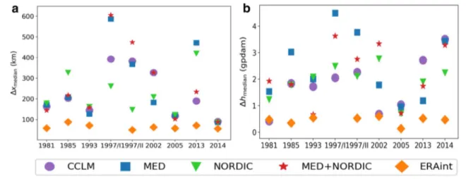
Fig. 5 a Median values of geodesic cyclone path distances ( Δxmedian)
and b core geopotential height differences ( Δhmedian) compared to
MERRA-2 reanalysis data for each event (colored symbols). Only
track points during the three consecutive extreme precipitation days (see Table 1) were chosen
The median of the geodesic distances and absolute dif-ferences in core geopotential heights for the cyclone tracks were calculated for the three consecutive days of highest precipitation (Table 1). For each event, the median of the geodesic distances between the simulated or ERA-Interim trajectories and those from MERRA-2 are summarized in Fig. 5a. Note that the temporal resolution of the ERA-Interim and MERRA-2 tracks is 6 h, while model data output was available at 3 h. Therefore, only every sec-ond model track point was used to calculate the median
Δxmedian of the geodesic distance deviations Δx from the reference tracks in the MERRA-2 reanalysis data. The medians Δxmedian for the ERA-Interim tracks are less than
100 km for all events. In most of the cases, the cyclone trajectories simulated in the coupled models are close to the controlled (CCLM) simulations. In July 1997 and August 2002, the coupled model performed better than the CCLM. The best-suited coupling set up (NORDIC, MED, or MED + NORDIC) varies from event to event according to the reference trajectories. This was also the
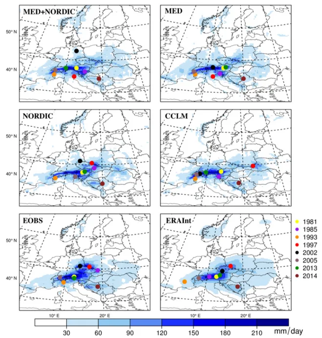
Fig. 6 Composite precipitation (mm/day) averaged over each event for three consecutive days (listed in Table 1) from all simulations, ERA-Interim, and observation E-OBS. Colored contours indicate the precipitation fields greater than 20 mm/day for each event
case for the core geopotential heights, which is a meas-ure of cyclone intensity and life cycle phase. Figmeas-ure 5b shows, analogous to Fig. 4, the medians Δhmedian of the
core geopotential height differences to the reference tracks (MERRA-2). Note that the average core geopotential heights of all MERRA-2 track points were approximately 296 geopotential decameter (gpdam). Thus, all medians Δh
median are approximately 1% of the average MERRA-2 core
geopotential height. Except for the August 2005 event, dif-ferences in the strengths of the simulated cyclones among the models are diverse. With the exception of 2013, in most of the cases the cyclone strengths differ most in the MED simulations compared to the reference. Overall, the uncoupled simulation based on ERA-Interim SST val-ues performs best. Among the different coupling set-ups, the coupling of the North and Baltic Seas improves the cyclone intensity and position most.
3.2.2 Precipitation
To evaluate the performance of the uncoupled and coupled models in simulating precipitation intensities associated with Vb-cyclones, we selected the three consecutive days of highest precipitation from each event (cf. Table 1). Figure 6 shows composite daily precipitation fields (averaged over 3 days for each event) of selected Vb-events for all model simulations, ERA-Interim reanalysis, and E-OBS. In most simulated events, precipitation mainly fell over the northern side of Alps and extended toward East and Central Europe following the cyclone trajectories (Fig. 4). During the decay-ing phase, the cyclone paths diverged, but most precipitation occurs during the intensification and mature phase. Thus, the later stage track divergence does not have a large influence on the simulated precipitation fields. The positions of the precipitation fields (Fig. 6) agreed well with the correspond-ing cyclone trajectories (Fig. 4). This is in contrast to the
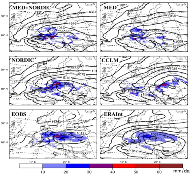
Fig. 7 Total precipitation (mm/day; colored contours) and mean sea level pressure (line contours) from all the simulations, ERA-Interim and
findings of Messmer et al. (2017), who found no relevant influence of cyclone tracks on changed precipitation fields due to changes in SST and soil moisture.
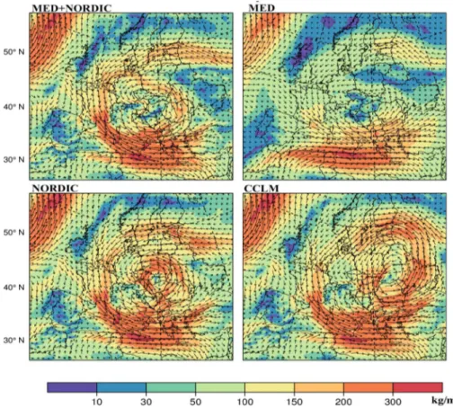
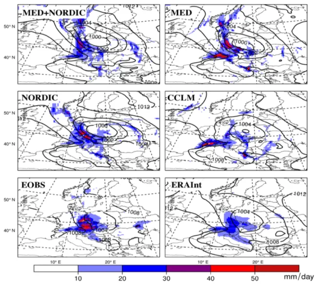
In most of the simulated events, the difference between the locations of the simulated precipitation fields are small except in the July 1997 and August 2002 events. As shown above, the cyclone tracks also differ among models in these events. In the July 1997 event, CCLM shifted the precipita-tion locaprecipita-tion eastward compared to the observaprecipita-tions. The simulated precipitation location in NORDIC is closer to the observed (Figs. 5a, 6). Figure 7 shows the total precipi-tation and mean sea level pressure for all the simulations, ERA-Interim, and E-OBS for the July 1997 event. The mean sea level pressure gradient is more intense in NORDIC and CCLM. However, the position of the cyclone in CCLM is shifted to the east. NORDIC shows strong moisture flux and anticyclonic wind with clear cyclone structure. The location of the cyclone is improved in MED + NORDIC and MED but the intensity is weaker than NORDIC. A similar result was also found by Ho-Hagemann 2015, where the coupling of the North and Baltic Seas improved the precipitation sim-ulation of the July 1997 event due to better pressure patterns and soil moisture conditions in the coupled simulations. Fig-ure 8 shows the vertically integrated moisture flux for the July 1997 event. In this case, NORDIC shows higher inland moisture flux than other simulations.
Figure 9 shows the total precipitation and mean sea level pressure for all the simulations, ERA-Interim, and E-OBS for the August 2002 event. The simulated precipitation loca-tion for the August 2002 event is better represented in MED. In this case, the mean sea level pressure simulated in CCLM is higher (4 hPa) than in the other simulations (Fig. 9). The moisture flux is stronger in the MED + NORDIC, NORDIC and CCLM simulations (Fig. 10), whereas the precipitation intensity and location is better represented in MED due to one clear structure which is split into two for other simula-tions. In general, all the coupled configurations captured the precipitation reasonably well in comparison to the controlled (CCLM) simulations, which uses reanalysis SST. The simu-lations for July 1981, August 1985, September 1993, August 2005, and May 2014 did not show large differences among different model configurations.
Figure 11 shows composite daily evaporation fields (aver-aged over 3 days for each event) of selected Vb-events for all model simulations and the ERA-Interim reanalysis. The Genoa region and Gulf of Lions play an important role in the contribution of moisture flux for Vb-cyclones. The coupling of the Mediterranean Sea generally shows less evaporation over the Gulf of Lions due to the cooling effect of the strong wind systems (Fig. 11). In the Mistral region, the evapora-tion is too strong in the NORDIC and CCLM.
Figure 12 shows the difference in mean precipitation (in a domain of 30 × 30 grid boxes centered on the E-OBS
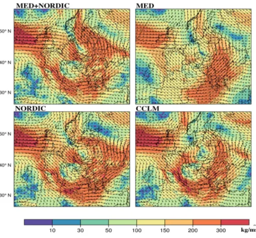
Fig. 8 Average vertically inte-grated moisture flux [kg/(ms); shaded and vector] from all the simulations for 18–20 July 1997
maximum for each event) between simulations and E-OBS. In most analyzed cases, differences among models are less than 1 mm/day, except in July 1997, August 2002, and May/ June 2013, when the simulated cyclone tracks also differ the most. Despite some differences, all the coupled configura-tions simulated the precipitation quite well compared to the controlled simulations (CCLM) and observations. Simulated precipitation is underestimated in most events, potentially due to coarse model grid-spacing (25 km in our case), which does not sufficiently resolve the orographic features and underestimates heavy convection in heavy Vb precipitation events. The object-based quality measure SAL (Wernli et al. 2008) was used in a more detailed analysis of daily ampli-tude, spatial shift, and structure of the precipitation fields.
Observed E-OBS precipitation fields were used as a reference. Figure 13 shows the SAL diagram for the three consecutive days of highest precipitation (Table 1) of the Vb-events. In the top left quadrant of the panels, the
amplitude is overestimated while the structure is underes-timated, indicating too much precipitation with too small or/and peaked objects. In the bottom left quadrant, both amplitude and structure are underestimated, indicating too low precipitation and too small or/and peaked objects. In the top right quadrant, both amplitude and structure are overestimated while in bottom right quadrant, amplitude is underestimated with too large or/and flat objects. Most simulated SA values are in the left half of the diagram, indicating too small or/and peaked precipitation objects. In most cases, ERA-Interim’s SA values are in the right half of the diagram, indicating too large or/and flat objects compared to E-OBS. Location component L is best (close to zero) for NORDIC and showed the highest number of days with precipitation values close to the observations (in the range of 0–0.1) (Fig. 13).
Table 2 summarizes the mean values of SAL compo-nents. Here, all models simulate too small or/and peaked
Fig. 9 Total precipitation (mm/day; colored contours) and mean sea level pressure (line contours) from all the simulations, ERA-Interim and E-OBS data for 11–13 July 1997
objects and have similar mean location errors. The largest inter-model scatter is simulated in the S component, which is best in MED + NORDIC and NORDIC. The ERA-Interim is poorest in the S component.
4 Conclusions
This study evaluated the robustness of a newly-developed regional atmosphere–ocean model, which incorporated cou-pling of two European marginal seas, the Mediterranean and North and Baltic Seas, to simulate Vb-cyclones, a weather phenomenon that often leads to intense precipitation over Central Europe. We investigated the impact of interactively simulated air-sea interactions and feedbacks over the Euro-pean marginal seas on the trajectories and intensities of Vb-cyclones.
We first evaluated the simulated SST. The results showed that the mean seasonal and annual SSTs simulated in MED + NORDIC are similar to MED for the Mediterranean Sea and to NORDIC for the North and Baltic Seas. Com-pared to uncoupled simulations or observations, SSTs simu-lated using the coupled configurations show biases (~ 1 °C) over the coupling regions, especially during winter and sum-mer. The coupled model configurations are stable and robust,
and the model’s SST uncertainties are promisingly small given the observational uncertainties in the marginal seas.
In general, all model configurations were able to repro-duce the trajectories of Vb-cyclones and their main fea-tures, such as trajectories and core geopotential heights compared to the reanalysis data. Cyclone positions scat-ter in the simulations with no configuration were best in all cases. Overall, the cyclone trajectories and core geo-potential heights are closest to the ERA-Interim reanalysis data in the uncoupled simulation driven by ERA-Interim SSTs. Among the coupling configurations, the coupling setup of the North and Baltic Seas shows smallest biases in simulating the cyclone trajectories and core geopoten-tial. The evaluation of the simulated precipitation fields revealed that all models were able to capture intense pre-cipitation patterns, but the patterns were peaked differently and shifted. The Mediterranean Sea coupling reduced the evaporation during the Vb-events over the Gulf of Lions due to cooling effect Vb-events, which can also affect the precipitation intensity. Generally, the simulated precipi-tation underestimated E-OBS precipiprecipi-tation data, possi-bly caused by the coarse model grid-spacing of 25 km, which does not sufficiently resolve orographic features and underestimates heavy convection in heavy Vb precipita-tion events.
Fig. 10 Average vertically integrated moisture flux [kg/ (ms); shaded and vector] from all the simulations for 11–13 August 2002
Because ERA-Interim’s OISST driven SSTs were applied in uncoupled sea areas, it is not surprising that no specific coupled configuration is closer to ERA-Interim than the uncoupled configuration in all cases. Additionally, coupling only the North and Baltic Seas showed an added value in simulating Vb-cyclones, especially in the July 1997 case, which is also shown in Ho-Hagemann (2015). This is due to the contribution of different moisture sources for each indi-vidual case (cf. Gimeno et al. 2010; Volosciuk et al. 2016; Messmer et al. 2017).
The results presented here indicate that a coupled sys-tem with two marginal seas is a useful tool for simulating regional climate over Europe and to study extreme events such as Vb-cyclones. Such a tool, with highly resolved and interactively simulated SSTs and high-frequency air–sea coupling over two main European marginal seas, can be useful for studying the pre-satellite era and future climate conditions. This coupled system with two marginal seas
Fig. 11 Composite evaporation (mm/day) averaged over each event for three consecutive days (listed in Table 1) from all simulations and ERA-Interim
Fig. 12 Mean precipitation difference compared to E-OBS over 3 days for each event, listed in Table 1
model is a step forward towards a high-resolution fully cou-pled regional climate system. Ongoing developments such as closing the water cycle with a river routing model and better grid resolution, will advance the coupled model shown here towards a convection-permitting regional climate system model.
Acknowledgements The authors would like to thank the Center for Scientific Computing (CSC) of the Goethe University Frankfurt am Main and the Deutsches Klimarechenzentrum (DKRZ) for providing computational facilities. B. Ahrens acknowledges support by Senck-enberg Biodiversity and Climate Research Centre (BiK-F), Frankfurt am Main. B. Ahrens and A. Krug acknowledge support by Deutsche Forschungsgemeinschaft (DFG, Research Unit For 2416: Space–Time Dynamics and Extreme Floods). B. Ahrens and N. Akhtar acknowledge support from the German Federal Ministry of Education and Research (BMBF) under grant MiKliP II (FKZ 01LP1518C). This work is part of the Med-CORDEX initiative (http://www.medco rdex.eu) supported by the HyMeX (https ://hymex .org/). We also thank Burkhardt Rockel (Helmholtz-Zentrum Geesthacht-HZG), Stefan Hagemann (HZG), Ha Hagemann (HZG) and Shakeel Asharaf (Jet Propulsion Laboratory) for fruitful discussions. We acknowledge the E-OBS dataset from the EU-FP6 project ENSEMBLES (http://ensem bles-eu.metoffi ce.com/) and the data providers in the ECA&D project (https ://www.ecad.eu/).
Fig. 13 SAL diagram for daily precipitation (the 3 days with high-est precipitation days per event) forecast for uncoupled and coupled models and ERA-Interim for the simulated Vb-events. The loca-tion of each dot shows the daily values of the S (Structure) and A (Amplitude) components, whereas the dot colors indicate the values
of L (Location). Dashed lines show the mean values for the S and A components, and gray boxes extend from the 20th–80th percentile of S and A, respectively. L_M and L_P represent the mean and 20th to 80th percentile values of the L component, respectively
Table 2 Average SAL values for selected cases with model simula-tions and ERA-Interim
A perfect coincidence with observation data is indicated by S-, A-, and L- values of 0
MED + NORDIC MED NORDIC CCLM ERAInt
S − 0.101 − 0.197 − 0.083 − 0.167 0.523
A − 0.030 0.002 − 0.020 − 0.003 0.006
Open Access This article is distributed under the terms of the Crea-tive Commons Attribution 4.0 International License (http://creat iveco mmons .org/licen ses/by/4.0/), which permits unrestricted use, distribu-tion, and reproduction in any medium, provided you give appropriate credit to the original author(s) and the source, provide a link to the Creative Commons license, and indicate if changes were made.
References
Akhtar N, Brauch J, Dobler A, Béranger K, Ahrens B (2014) Medicanes in an ocean-atmosphere coupled regional climate model. Nat Haz-ards Earth Syst Sci 14:2189–2201. https ://doi.org/10.5194/nhess -14-2189-2014
Akhtar N, Brauch J, Ahrens B (2018) Climate Modeling over the Medi-terranean Sea: impact of resolution and ocean coupling. Clim Dyn 51:933. https ://doi.org/10.1007/s0038 2-017-3570-8
Alpert P, Stein U, Tsidulko M (1995) Role of sea fluxes and topogra-phy in eastern Mediterranean cyclogenesis. Global Atmos Ocean Syst 3:55–79
Artale V, Calmanti S, Carillo A, Dell’Aquila A, Herrmann M, Pisacane G, Ruti PM, Sannino G, Struglia MV, Giorgi F, Bi X, Pal JS, Rauscher S, The PROTHEUS Group (2010) An atmosphere– ocean regional climate model for the Mediterranean area: assess-ment of a present climate simulation. Clim Dyn 35:721–740. https ://doi.org/10.1007/s0038 2-009-0691-8
Awan NK, Formayer H (2016) Cut-off low systems and their rele-vance to large-scale extreme precipitation in the European Alps. Theor Appl Climatol 129:149–158. https ://doi.org/10.1007/s0070 4-016-1767-0
Balmaseda MA, Mogensen K, Weaver AT (2013) Evaluation of the ECMWF ocean reanalysis system ORAS4. Q J R Meteorol Soc 139:1132–1161. https ://doi.org/10.1002/qj.2063
Bebber V (1891) Die Zugstrassen der barometrischen Minima nach den Bahnenkarten der Deutschen Seewarte für den Zeitraum 1875–1890. Meteorol Z 8:361–366
Beniston M (2006) August 2005 intense rainfall event in Switzer-land: not necessarily an analog for strong convective events in a greenhouse climate. Geophys Res Lett 33:L05701. https ://doi. org/10.1029/2005G L0255 73
Beuvier J, Béranger K, Lebeaupin C, Somot S, Sevault F, Drillet Y, Bourdall.-Badie R, Ferry N, Lyard F (2012) Spreading of the Western Mediterranean Deep water after winter 2005: time scales and deep cyclone transport. J Geophys Res 117:50. https ://doi. org/10.1029/2011j c0076 79
Christensen JH, Christensen O (2007) A summary of the PRUDENCE model projections of changes in European climate by the end of this century. Clim Change 81(1):7–30. https ://doi.org/10.1007/ s1058 4-006-9210-77-30
Craig A, Valcke S, Coquart L (2017) Development and performance of a new version of the OASIS coupler, OASIS3-MCT_3.0. Geosci Model Dev Discuss 45:50. https ://doi.org/10.5194/gmd-2017-64 Cyberski J, Grzes M, Gutry-Korycka M, Nachlik E, Kundzewicz
ZW (2006) History of floods on the River Vistula. Hydrol Sci J 51:799817. https ://doi.org/10.1623/hysj.51.5.799
Dee DP, Uppala SM, Simmons AJ, Berrisford P, Poli P, Kobayashi S, Andrae U, Balmaseda MA, Balsamo G, Bauer P, Bechtold P, Beljaars ACM, van de Berg L, Bidlot J, Bormann N, Delsol C, Dragani R, Fuentes M, Geer AJ, Haimberger L, Healy SB, Hers-bach H, Hólm EV, Isaksen L, Kållberg P, Köhler M, Matricardi M, McNally AP, Monge-Sanz BM, Morcrette JJ, Park BK, Peubey C, de Rosnay P, Tavolato C, Thépaut JN, Vitart F (2011) The ERA-Interim reanalysis: configuration and performance of the
data assimilation system. Q J R Meteorol Soc 137:553–597. https ://doi.org/10.1002/qj.828
Denis B, Côté J, Laprise R (2002) Spectral decomposition of two-dimensional atmospheric fields on limited-area domains using the discrete cosine transform (DCT). Mon Weather Rev 130:1812– 1829. https ://doi.org/10.1175/1520-0493(2002)130%3c181 2:SDOTD A%3e2.0.CO;2
Dieterich C, Schimanke S, Wang S, Väli G, Liu Y, Hordoir R, Axell L, Meier H (2013) Evaluation of the SMHI coupled atmosphere-ice-ocean model RCA4-NEMO. Tech Rep 47, Swedish Meteorologi-cal and HydrologiMeteorologi-cal Institute (SMHI), Sweden
Egbert GD, Erofeeva SY (2002) Efficient inverse modeling of baro-tropic ocean tides. J Atmos Ocean Technol 19:183–204. https ://doi.org/10.1175/1520-0426(2002)019%3c018 3:EIMOB O%3e2.0.CO;2
Egbert GD, Erofeeva SY, Ray RD (2010) Assimilation of altimetry data for nonlinear shallow-water tides: quarter-diurnal tides of the Northwest European Shelf. Cont Shelf Res 30(6):668–679. https ://doi.org/10.1016/j.csr.2009.10.011
Gangoiti G, Sáez de Cámara E, Alonso L, Navazo M, Gómez MC, Iza J, García JA, Ilardia JL, Millán MM (2011) Origin of the water vapor responsible for the European extreme rainfalls of August 2002: 1. High resolution simulations and tracking of air masses. J Geophys Res Atmos 116:D21102. https ://doi.org/10.1029/2010j d0155 30
Gelaro R, McCarty W, Suárez MJ, Todling R, Molod A, Takacs L, Ran-dles CA, Darmenov A, Bosilovich MG, Reichle R, Wargan K, Coy L, Cullather R, Draper C, Akella S, Buchard V, Conaty A, da Silva AM, Gu W, Kim G, Koster R, Lucchesi R, Merkova D, Nielsen JE, Partyka G, Pawson S, Putman W, Rienecker M, Schubert SD, Sienkiewicz M, Zhao B (2017) The Modern-Era retrospective analysis for research and applications, version 2 (MERRA-2). J Clim 30:5419–5454. https ://doi.org/10.1175/JCLI-D-16-0758.1 Gimeno L, Drumond A, Nieto R, Trigo RM, Stohl A (2010) On the
origin of continental precipitation. Geophys Res Lett 37:L13804. https ://doi.org/10.1029/2010G L0437 12
Giorgi F (2006) Climate change hot-spots. Geophys Res Lett 33:L08707. https ://doi.org/10.1029/2006G L0257 34
Giorgi F, Jones C, Asrar GR (2006) Addressing climate information needs at the regional level: the CORDEX framework. World Mete-orol Bull 58:175–183
Graefe H and Hegg (2004) Ereignisanalyse Hochwasser August 2002 in den Osterzgebirgsüssen. Tech rep Säachsisches Landesamt für Umwelt und Geologie, 176 pp
Godina R, Lalk P, Lorenz P, Müller G, Weilguni, V (2006) Hochwasser 2005. Ereignisdokumentation: Teilbericht des Hydrographischen Dienstes, Federal Ministry for Agriculture, Forestry, Environment and Water Management, Sekt. VII, Vienna, 30 p
Grams CM, Binder H, Pfahl S, Piaget N, Wernli H (2014) Atmospheric processes triggering the central European floods in June 2013. Nat Hazards Earth Syst Sci 14:1691–1702. https ://doi.org/10.5194/ nhess -14-1691-2014
Grazzini F, van der Grijn G (2002) Central European floods during summer 2002. ECMWF Newslett 96:18–28
Gröger M, Dieterich C, Meier HEM, Schimanke S (2015) Thermal air–sea coupling in hindcast simulations for the North Sea and Baltic Sea on the NW European shelf. Tellus A. https ://doi. org/10.3402/tellu sa.v67.26911
Haylock MR, Hofstra H, Klein Tank AMG, Klok EJ, Jones PD, New M (2008) A European daily high resolution gridded dataset of surface temperature and precipitation. J Geophys Res Atmos 113:D20119. https ://doi.org/10.1029/2008J D1020 1
Held H, Gerstengarbe F-W, Pardowitz T, Pinto JG, Ulbrich U, Born K, Donat MG, Karremann MK, Leckebusch GC, Ludwig P, Nis-sen KM, Österle H, Prahl BF, Werner PC, Befort DJ, Burghoff
O (2013) Projections of global warming-induced impacts on winter storm losses in the German private household sector. Clim Change 121:195–207. https ://doi.org/10.1007/s1058 4-013-0872-7
Herrmann M, Somot S (2008) Relevance of ERA40 dynamical down-scaling for modeling deep convection in the North-Western Mediterranean Sea. Geophys Res Lett 35:L0460. https ://doi. org/10.1029/2007G L0324 42
Herrmann M, Somot S, Calmanti S, Dubois C, Sevault F (2011) Repre-sentation of daily wind speed spatial and temporal variability and intense wind events over the Mediterranean Sea using dynamical 594 downscaling: impact of the regional climate model configu-ration. Nat Hazards Earth Syst Sci 11:1983–2001. https ://doi. org/10.5194/nhess -11-1983-201
Hofstätter M, Chimani B (2012) Van Bebber’s cyclone tracks at 700 hPa in the Eastern Alps for 1961–2002 and their comparison to circulation type classifications. Meteorol Z 21:459–473. https ://doi.org/10.1127/0941-2948/2012/0473
Hofstätter M, Chimani B, Lexer A, Blöschl G (2016) A new clas-sification scheme of European cyclone tracks with relevance to precipitation. Water Resour Res 52:7086–7104. https ://doi. org/10.1002/2016W R0191 46
Hofstätter M, Lexer A, Homann M, Blöschl G (2018) Large-scale heavy precipitation over central Europe and the role of atmos-pheric cyclone track types. Int J Climatol 38:497–517. https :// doi.org/10.1002/joc.5386
Ho-Hagemann H (2015) On the role of soil in the generation of heavy rainfall during the Oder flood event in July 1997. Tellus A 67:28661. https ://doi.org/10.3402/tellu sa.v67.28661
Hoskins B, Hodges K (2002) New perspectives on the Northern Hemi-sphere winter storm tracks. J Atmos Sci 59:1041–1061. https :// doi.org/10.1175/1520-0469(2002)059<1041:NPOTN H>2.0.CO;2 IPCC (2007) Climate change 2007: the physical science basis-IPCC
working group 1 contribution to AR4. Tech. rep., Intergovernmen-tal Panel on Climate Change, Cambridge, United Kingdom and New York, NY, USA, 996 p
IPCC (2013) Climate Change 2013: The Physical Science Basis. Con-tribution of Working Group I to the Fifth Assessment Report of the Intergovernmental Panel on Climate Change. Cambridge Uni-versity Press, Cambridge, United Kingdom and New York, NY, USA, 1535 p
James P, Stohl A, Spichtinger N, Eckhardt S, Forster C (2004) Clima-tological aspects of the extreme European rainfall of August 2002 and a trajectory method for estimating the associated evaporative source regions. Nat Hazards Earth Syst Sci 4:733–746. https ://doi. org/10.5194/nhess -4-733-2004
Janssen F, Schrum C, Backhaus JO (1999) A climatological data set of temperature and salinity for the Baltic Sea and the North Sea, Hydrographische Zeitschrift German. J Hydrogr Suppl 51:245 Kaspar M, Müller M (2008) Selection of historic heavy large-scale
rainfall events in the Czech Republic. Nat Hazards Earth Syst Sci 8:1359–1367. https ://doi.org/10.5194/nhess -8-1359-2008 Kelemen F, Ludwig P, Reyers M, Ulbrich S, Pinto J (2016)
Evalua-tion of moisture sources for the Central European summer flood of May/June 2013 based on regional climate model simulations. Tellus A. https ://doi.org/10.3402/tellu sa.v68.29288
Lebeaupin C, Béranger K, Deltel C, Drobinski P (2011) The Mediter-ranean response to different space-time resolution atmospheric forcings using perpetual mode sensitivity simulations. Ocean Model 36:1–25. https ://doi.org/10.1016/j.ocemo d.2010.10.008 Lebeaupin C, Béranger K, Drobinski P (2012) Sensitivity of the
north-western Mediterranean Sea coastal and thermohaline circulations simulated by the 1/12°-resolution ocean model NEMOMED12 to the spatial and temporal resolution of atmospheric forcing. Ocean Model 43–44:94–107. https ://doi.org/10.1016/j.ocemo d.2011.12.007
Lehmann A, Myrberg K (2008) Upwelling in the Baltic Sea: a review. J Mar Syst 74:53. https ://doi.org/10.1016/j.jmars ys.2008.02.010 Levitus S, Antonov J, Boyer T (2005) Warming of the world
ocean 1955–2003. Geophys Res Lett 32:L02604. https ://doi. org/10.1029/2004G L0215 92
Li L (2006) Atmospheric GCM response to an idealized anomaly of the Mediterranean Sea surface temperature. Clim Dyn 27:543–552. https ://doi.org/10.1007/s0038 2-006-0152-6
Lindström G, Pers CP, Rosberg R, Strömqvist J, Arheimer B (2010) Development and test of the HYPE (Hydrological Predictions for the Environment) model: a water quality model for different spatial scales. Hydrol Res 41:295–319. https ://doi.org/10.2166/ nh.2010.007
Ludwig W, Dumont E, Meybeck M, Heussner S (2009) River dis-charges of water and nutrients to the Mediterranean Sea: major drivers for ecosystem changes during past and future decades? Prog Oceanogr 80:199–217. https ://doi.org/10.1016/j.pocea n.2009.02.001
Madec G, the NEMO Team (2008) NEMO Ocean Engine, Note Pôle Modél, 27. Inst Pierre-Simon Laplace, Paris
Meier H, Kauker F (2003) Modeling decadal variability of the Baltic Sea: 2. Role of freshwater inflow and large-scale atmospheric cir-culation for salinity. J Geophys Res 108(C11):3368. https ://doi. org/10.1029/2003j c0017 97
Messmer M, Gómez-Navarro JJ, Raible CC (2015) Climatology of Vb cyclones, physical mechanisms and their impact on extreme precipitation over Central Europe. Earth Syst Dyn 6:541–553. https ://doi.org/10.5194/esd-6-541-2015
Messmer M, Gómez-Navarro JJ, Raible CC (2017) Sensitivity experi-ments on the response of Vb cyclones to sea surface temperature and soil moisture changes. Earth Syst Dyn 8:477–493. https ://doi. org/10.5194/esd-8-477-2017
MeteoSchweiz (2006) Starkniederschlagsereignis August 2005 Arbe-itsberichte der Schweiz, 211, 63 p
Mitzschke H (2013) Gewässerkundlicher Monatsbericht mit vorläufiger Auswertung des Hochwassers. Tech. rep., Sächsisches Landesamt für Umwelt, Landwirtschaft und Geologie, 69 p
Mudelsee M, Borngen M, Tetzlaff G, Grunewald U (2004) Extreme floods in Central Europe over the past 500 years: role of cyclone pathway Zugstrasse Vb. Geophys Res 109(D23):101. https ://doi. org/10.1029/2004J D0050 34
Muskulus M, Jacob D (2005) Tracking cyclones in regional model data: the future of Mediterranean storms. Adv Geosci 2:13–19 Nied M, Pardowitz T, Nissen K, Uwe U, Hundecha Y, Merz B (2014)
On the relationship between hydro-meteorological patterns and flood types. J Hydrol 519:3249–3262. https ://doi.org/10.1016/j. jhydr ol.2014.09.089
Nissen KM, Leckebusch GC, Pinto JG, Ulbrich U (2013) Mediter-ranean cyclones and windstorms in a changing climate. Reg Environ Change 14:1873–1890. https ://doi.org/10.1007/s1011 3-012-0400-8
Osiński R, Rak D, Walczowski W, Piechura J (2010) Baroclinic Rossby radius of deformation in the southern Baltic Sea. Oceanologia 52(3):417–429
Petterssen S (1956) Weather Analysis and Forecasting. Mac Graw Hill, New York
Pham VT, Brauch J, Dieterich C, Frueh B, Ahrens B (2014) New cou-pled atmosphere-ocean-ice system COSMO-CLM/NEMO: on the air temperature sensitivity on the North and Baltic Seas. Oceano-logia 56:167–189. https ://doi.org/10.5697/oc.56-2.167
Reynolds WR, Smith TM, Liu C, Chelton DB, Casey KS, Schlax MG (2007) Daily high-resolution-blended analyses for sea surface temperature. J Clim 20:5473–5496. https ://doi.org/10.1175/2007J CLI18 24.1
Ritter B, Geleyn J-F (1992) A comprehensive radiation scheme for numerical weather prediction models with potential applications
in climate simulations. Mon Weather Rev 120(2):303–325. https ://doi.org/10.1175/1520-0493(1992)120%3c030 3:ACRSF N%3e2.0.CO;2
Rixen M (2012) MEDAR/MEDATLAS-II, GAME/CNRM. https ://doi. org/10.6096/hymex .medar /medat las-ii.20120 112
Rixen M, Beckers J, Levitus S, Antonov J, Boyer T, Maillard C, Fichaut M, Balopoulos E, Iona S, Dooley H, Garcia M, Manca B, Giorgetti A, Manzella G, Mikhailov N, Pinardi N, Zavatarelli M (2005) The Western Mediterranean Deep Water: a proxy for climate change. Geophys Res Lett 32(12):L12608. https ://doi. org/10.1029/2005G L0227 02
Robinson AR, Golnaraghi M (1993) Circulation and dynamics of the eastern Mediterranean Sea: quasi-synoptic data-driven simula-tions. Deep Sea Res II 40:1207–1246
Rockel B, Will A, Hense A (2008) The regional climate model COSMO-CLM (CCLM). Meteorol Z 17:347–348. https ://doi. org/10.1127/0941-2948/2008/0309
Ruti PM, Somot S, Giorgi F, Dubois C, Flaounas E, Obermann A, Dell’Aquila A, Pisacane G, Harzallah A, Lombardi E, Ahrens B, Akhtar N, Alias A, Arsouze T, Aznar R, Bastin S, Bartholy J, Béranger K, Beuvier J, Bouffies-Cloché S, Brauch J, Cabos W, Calmanti S, Calvet J-C, Carillo A, Conte D, Coppola E, Djurd-jevic V, Drobinski P, Elizalde-Arellano A, Gaertner M, Galàn P, Gallardo C, Gualdi S, Goncalves M, Jorba O, Jordà G, L’Heveder B, Lebeaupin-Brossier C, Li L, Liguori G, Lionello P, Maciàs- Moy D, Nabat P, Onol B, Rajkovic B, Ramage K, Sevault F, Sannino G, Struglia MV, Sanna A, Torma C, Vervatis V (2016) MED-CORDEX initiative for Mediterranean Climate studies. Bull Am Meteorol Soc. https ://doi.org/10.1175/bams-d-14-00176 .1
Sanchez-Gomez E, Somot S, Josey SA, Dubois C, Elguindi N et al (2011) Evaluation of Mediterranean Sea water and heat budgets simulated by an ensemble of high resolution regional climate models. Clim Dyn 37:2067–2086. https ://doi.org/10.1007/s0038 2-011-1012-6
Sanna A, Lionello P, Gualdi S (2013) Coupled atmosphere ocean cli-mate model simulations in the Mediterranean region: effect of a high resolution marine model on cyclones and precipitation. Nat Hazards Earth Syst Sci 13:1567–1577. https ://doi.org/10.5194/ nhess -13-1567-2013
Sodemann H, Wernli H, Schwierz C (2009) Sources of water vapour contributing to the Elbe flood in August 2002: a tagging study in a mesoscale model. Q J R Meteorol Soc 135:205–223. https ://doi.org/10.1002/qj.374
Somot S, Sevault F, Déqué M (2008) 21st century climate change scenario for the Mediterranean using a coupled atmosphere-ocean regional climate model. Global Planet Change 63:112– 126. https ://doi.org/10.1016/j.glopl acha.2007.10.003
Stadtherr L, Coumou D, Petoukhov V, Petri S, Rahmstorf S (2016) Record Balkan floods of 2014 linked to planetary wave reso-nance. Sci Adv 2(4):e1501428. https ://doi.org/10.1126/sciad v.15014 28
Stohl A, James P (2004) A Lagrangian analysis of the atmospheric branch of the global water cycle, Part I: method description,
validation, and demonstration for the August 2002 flood-ing in Central Europe. J Hydrometeorol 5:656–678. https ://doi.org/10.1175/1525-7541(2004)005%3c065 6:ALAOT A%3e2.0.CO;2
Stucki P, Martius O, Brönnimann S, Franke J (2013) The extreme flood event of Lago Maggiore in September 1993. In: Brönni-mann S, Martius O (eds) Weather extremes during the past 140 years. Geographica Bernensia G89, Bern, pp 53–58. https ://doi. org/10.4480/gb201 3.g89.06
Tegen I, Hoorig P, Chin M, Fung I, Jacob D, Penner J (1997) Contri-bution of different aerosol species to the global aerosol extinc-tion optical thickness: estimates from model results. J Geophys Res 102(23):23895–23915. https ://doi.org/10.1029/97jd0 1864 Ulbrich U, Brücher T, Fink AH, Leckebusch GC, Krüger A, Pinto JG
(2003a) The central European floods of August 2002: Part 1– Rainfall periods and flood development. Weather 58:371–377. https ://doi.org/10.1256/wea.61.03A
Ulbrich U, Brücher T, Fink AH, Leckebusch GC, Krüger A, Pinto JG (2003b) The central European floods of August 2002: Part 2–Synoptic causes and considerations with respect to cli-matic change. Weather 58:434–442. https ://doi.org/10.1256/ wea.61.03B
Vancoppenolle M, Fichefet T, Goosse H, Bouillon S, Madec G, Maqueda M (2009) Simulating the mass balance and salinity of arctic and Antarctic sea ice. Ocean Model 27:33–53. https :// doi.org/10.1016/j.ocemo d.2008.10.005
Volosciuk C, Maraun D, Vladimir AS, Tilinina N, Gulev SK, Latif M (2016) Rising Mediterranean sea surface temperatures amplify extreme summer precipitation in Central Europe. Sci Rep 6(1):32450. https ://doi.org/10.1038/srep3 2450
Wernli H, Schwierz C (2006) Surface cyclones in the ERA-40 data-set (1958–2001). Part I: novel identification method and global climatology. J Atmos Sci 63:2486–2507. https ://doi.org/10.1175/ JAS37 66.1
Wernli H, Paulat M, Hagen M, Frei C (2008) SAL: a novel quality measure for the verification of quantitative precipitation forecasts. Mon Weather Rev 136:4470–4487. https ://doi.org/10.1175/2008M WR241 5.1
Will A, Akhtar N, Brauch J, Breil M, Davin E, Ho-Hagemann HTM, Maisonnave E, Thürkow M, Weiher S (2017) The COSMO-CLM 4.8 regional climate model coupled to regional ocean, land surface and global earth system models using OASIS3-MCT: description and performance. Geosci Model Dev 10:1549–1586. https ://doi. org/10.5194/gmd-10-1549-2017
Winschall A, Sodemann H, Pfahl S, Wernli H (2014) How impor-tant is intensified evaporation for Mediterranean precipitation extremes? J Geophys Res Atmos 119:5240–5256. https ://doi. org/10.1002/2013J D0211 75
Publisher’s Note Springer Nature remains neutral with regard to jurisdictional claims in published maps and institutional affiliations.