CONTROLLING CACHE PARTITIONSIZES TO INCREASE APPLICATIONRELIABILITY

(1)

V¨

aster˚

as, Sweden

Undergraduate Thesis

CONTROLLING CACHE PARTITION

SIZES TO INCREASE APPLICATION

RELIABILITY

Janne Suuronen

jsn15011@student.mdh.se

Jawid Nasiri

jni15001@student.mdh.se

Examiner: Masoud Daneshtalab

Supervisor: Jakob Danielsson

(2)

as cache contention. Cache contention can negatively affect process reliability, since it can increase execution time jitter. Cache contention may be caused by inter-process interference in a system. To minimize the negative effects of inter-process interference, cache memory can be partitioned which would isolate processes from each other.

In this work, two questions related to cache-coloring based cache partition sizes have been inves-tigated. The first question is how we can use knowledge of execution characteristics of an algorithm to create adequate partition sizes. The second question is to investigate if sweet spots can be found to determine when cache-coloring based cache partitioning is worth using. The investigation of the two questions is conducted using two experiments. The first experiment put focus on how static partition sizes affect process reliability and isolation. The second experiment investigates both questions by using L3 cache misses caused by a running process to determine partition sizes dynamically.

Results from the first experiment shows static partition sizes to increase process reliability and isolation compared to a non-isolated system. The second experiment outcomes shows the dynamic partition sizes to provide even better process reliability compared to the static approach. Collectively, all results have been fairly identical and therefore sweets spots could not be found. Contributions from our work is a cache partitioning controller and metrics showing the effects of static and dy-namic partitions sizes.

(3)

1 Introduction

Symmetric multiprocessor (SMP) are commonly used today due to their overall increased perfor-mance compared to uniprocessor architectures. While SMPs are beneficial in terms of perforperfor-mance, SMPs also comes with its own share of problems. One of these problems comes from how shared cache memory is organized and utilized in a SMP alongside employed eviction policies, also known as cache contention.

Cache contention occurs as consequence of unconstrained usage of shared cache memory. Since all cores in a SMP system have access to the shared cache memory, they compete for available capacity. If the issue of cache contention is left unmanaged, system performance can be negatively effected as the Least Recently Used(LRU) eviction policy may evict stored data which is about to be used. This performance impact can become more troublesome if executing processes are time-critical, since execution time is affected by eventual cache misses.

One solution to solve the cache contention problem is to use cache partitioning, which splits cache memory into different independent partitions. This enables processes to execute isolated from each other and it can minimize risks of inter-core interference.

In this study we will investigate a cache partitioning method and determine if it can be used to increase process reliability. In combination with the cache partitioning method we employ different cache sizing approaches to investigate how they affect process reliability. Finally, we investigate cache partitioning to try determine sweet-spots, for when cache partitioning is worth using.

2 Background

This section will cover the concepts relevant to understand our work. Firstly, we explain symmetric multiprocessors, followed by explaining the SMP cache hierarchy used in our test system. We also cover cache misses and cache contention. This followed by an explanation of cache partitioning and cache-coloring. Finally, we cover Linux control groups (CGROUPS).

2.1 Symmetrical Multi-processors

Symmetrical multi-processors (SMP) consists of a single chip with multiple identical processing elements embedded onto it, also known as cores[1]. All cores use shared primary memory, DRAM. As each core is identically designed in an SMP, every core can perform the same kind of work as any other core on the same chip. Since cores are independent processing elements, they can execute multiple instructions in parallel, which makes it possible for SMPs to outperform single-core architectures. However, this is partially depending on how well a program can be parallelized.

2.2 Cache hierarchies in SMP

Cache hierarchies employed by SMP are often structured into different levels, which can either be private or shared between different cores [1]. In our work we have used a 3 level cache hierarchy, which consists of a private L1 and L2 cache followed by a shared L3 cache. An example of a 3 level cache hierarchy is illustrated in figure 1.

(6)

Figure 1: Example of three-leveled cache hierarchy.

The L1 cache is closest to the processor and is often smallest compared to other levels in a cache hierarchy. While being the smallest in terms of capacity, it makes up for being the fastest cache since it is physically placed closest to the processor. Internally, L1 is often split into two components: an instruction cache (IC) and a data cache (DC). IC stores incoming CPU instructions from higher levels and DC stores the data to used in CPU instructions.

The L2 cache is found between the L1 cache and the L3 cache. The L2 size is often larger compared to the L1 and can store data and instructions. However, since the L2 cache is placed a longer distance from the processor it is slower than the L1 cache. Similarly to L1, L2 is often private.

Finally, the L3 cache is the highest level in the illustrated cache hierarchy. L3 is also known as last-level cache (LLC) as it is the level before main memory in the illustrated hierarchy. Since the L3 cache is closest to the main memory it handles data transfers from main memory into the cache hierarchy. L3 is larger than L1 and L2, but is placed at a longer distance from the processor and therefore also slower than the L1 and L2 caches. In contrast to L1 and L2, L3 is shared among cores in an SMP.

2.3 Cache misses and cache contention

When the CPU needs data, a data request to cache is issued, which searches the caches for the address tag of the requested data [2]. If requested data is found in the caches a cache hit has occurred, if data is not found a cache miss has occurred [2], [3], [1].

In the previous example of a three-leveled cache hierarchy in figure 1 there is one shared cache level.

Shared caches can improve the performance of the cache but also decrease it. With a shared LLC a process can accidentally evict data belonging to another process according to an eviction

(7)

policy. This behavior is known as cache thrashing and is the result of the competition of cache lines between cores in a shared cache. [4]

2.4 Least Recently Used Policy

When cache misses occur and the cache is full, stored data must be evicted to make place for newly requested data. A commonly used policy dictating the eviction process is the Least recently used (LRU) policy. The basic concept of the LRU policy is to evict cache lines which was used least recently. The idea is based of the principal of temporal locality, since cache lines which have not been used lately will less likely be used again. When applying the mentioned concept, LRU sees the cache as a stack of memory blocks[5]. Blocks frequently used will be at the top of the stack and least used blocks at the bottom. Once a cache eviction is to be performed, blocks at the bottom of the stack are chosen as victims.

On a more detailed level, LRU uses status bits to track memory block usage in a cache[2]. Status bits are used to defer the time since a block has last been used, therefore it can determine which cache line should be victimized. The number of bits used to represent last usage is proportional to the degree of set-associativity in a cache. This means LRU becomes more difficult to implement in caches with high grades of set-associativity [1].

2.5 Cache-Partitioning

A way of organizing CPU cache is to use cache partitioning. Conceptually, cache partitioning involves division of a cache into different partitions[6]. The end-goal with cache partitioning is to minimize amount of inter-process interference which can occur within an SMP. Interference being the behavior where different processes access and use each others cache space. As a result of interference, a process may potentially cause cache misses when other processes access their data. A commonly used methodology for creating and assigning the partitions is to simply as-sign a partition to a given process[6]. By assigning partitions to a given process, processes are guaranteed to not fall victim of inter-process interference. Other options for partition creation are available, as described in ”Semi-Partitioned Hard-Real-Time Scheduling under Locked Cache Migration in Multicore Systems” and ”An adaptive bloom filter cache partitioning scheme for multicore architectures” [7], [8].

Cache partitioning relies on two connected parts, a partition mechanism and a partition policy [9]. The partition mechanism ensures processes are sticking to their assigned partitions. The partition policy specifies how partitions should be created, based of what rules partitions should be assigned and created. These parts combined ensures processes can execute without inter-process interference and are useful for time-critical tasks, where execution time is constrained [6].

2.6 Cache-Coloring

A software approach to cache partitioning is cache-coloring, which affects the translation process between virtual and physical pages[10]. Cache-coloring also affects how the physical pages stand in relation to cache lines. Page translation using cache coloring makes sure processes are not mapped to the same cache sets in shared cache. Consequently, processes are hindered from evicting each others data stored in cache. Figure 2 shows an example of how physical pages are mapped to the cache memory.

(8)

Figure 2: Cache colored translation from physical pages to cache sets [11, Fig. 2]

Cache-coloring also lowers the amount of inter-process interference which occurs in a system. The trick used is to label virtual and physical pages with colors, so only a given color can be mapped to matching physical pages and matching colored cache set. The number of colors a system can support is determined by equation (1) [11].

numberof colors = cachesize

numberof ways × pagesize (1)

Equation (1) is more apparent as colors are identified using color bits[11] in a memory address. More specifically, the color bits are the most significant bits of the cache set index bits. If memory addresses have different color bits, they also have different cache set indexes. Therefore, by having different color bits, memory addresses are guaranteed to map to different cache sets. Figure 3 shows an example of the color bits in a physical memory address.

(9)

Figure 3: Color bits in a physical memory address, p bits are used for the physical page offset [11, Fig. 1]

2.7 Cgroups - Linux control groups

Control groups are a Linux feature which allows system resources to be partitioned [12]. A partition in control cgroups is dictated by a hierarchy which is located in the cgroup pseudo file-system. Each hierarchy consists of subsystems which represent the different system resources a hierarchy is limited to. It is also in these hierarchy subsystem limits are specified, limits in this case can refer to amount of CPU time or memory a cgroup is allowed to use. Cgroups are collections of processes assigned to a control cgroup hierarchy. Concretely, a cgroup is simply a collection of relevant processes IDs (PIDS) which are limited to a control cgroup hierarchy.

The composition of a hierarchy is divided into multiple files, the subsystems which integer values are assigned to [12]. We cover only the cpuset.cpus, cpuset.mems and the group.procs files since remainder files are out-of-scope as they are not used. The cpuset.cpus and cpuset.mems files limits what CPUs and memory nodes a control cgroups is allowed to use. Cpuset.cpus contains the physical IDs of allowed to use CPUs/cores, and the cpuset.mems contains the ID of memory nodes allowed to use. A memory node in this case refers to a portion of memory in a Non-uniform memory access (NUMA) system[13], non-NUMA systems will have memory node 0 per default. Finally, the group.procs file contains the process IDs (PIDS) which make up a cgroup affected by defined resource limits.

3 Related Work

Cache partitioning and cache coloring are not new research areas, but work is still being done in respective area. In this section we present related works and put them into relation with our work. We also discuss weak and strong points with our work, compared to other authors work.

3.1 COLORIS

”COLORIS: a dynamic cache partitioning system using page coloring” by Y. Ye, R. West, Z. Cheng and Y. Le. Y. Ye et al. formulates a methodology which allows for static and dynamic cache partitioning using cache-coloring [11]. Essentially, the methodology employs different page colors for different cores, and different processes are assigned different colors on different cores. As such partitioning of cache is established using cache coloring.

Our work compared with the work by Y. Ye et al. we also apply cache coloring as base for our controller, but we also extend further on this base and add a cache miss partitioning heuristic. In our work we also make use of only dynamic partitioning when it comes to our controller, and use static partitioning purely for comparative reasons. E.g. to investigate if our controller performs better than static fair cache partitioning. But the source code for COLORIS is not open, therefore, while similar methods are employed, we do not explicitly expand on COLORIS.

(10)

3.2 PALLOC: DRAM Bank-Aware Memory Allocator for Performance

Isolation on Multicore Platforms

A work authored by H. Yun, R. Mancusom Z-P. Wu and R. Pellizzoni [14] uses dynamic DRAM bank partitioning combined with cache partitioning. H. Yun et al. formulates their methodology with the motivation that commercial-of-the-shelf (COTS) multi-core platforms tend to have an unpredictable memory performance. According to H. Yun et al. the cause is shared DRAM banks between all cores, even if executing programs do not share the same memory space. The solution H. Yun et al. proposes is a kernel-level memory allocator called Palloc, which dynamically partitions DRAM banks. H. Yun et al. suggest by partitioning DRAM banks, the issue of poor memory performance with shared DRAM banks is avoided. DRAM bank partitioning in Palloc is performed by setting a mask that specifies the DRAM bank bits in a physical memory address. The DRAM bank bits may overlap with cache set index bits, depending on which bits are used by DRAM banks. By setting overlapping bits H. Yun et al. means Palloc also partitions a limited portion of cache memory. With this effect taken into account, H. Yun et al. also investigates if cache partitioning combined with DRAM bank partitioning increases process reliability and real-time performance.

This is the primary work we extend upon in our thesis. We use Palloc as base for our work and our implementation. However, we do not use DRAM bank partitioning, instead we only use cache partitioning by only setting cache index set index bits in the mask. This taken into account, we only investigate effects of cache partitioning on process isolation and execution time stability.

3.3 Towards Practical Page Coloring-based Multi-core Cache

Manage-ment

An partial cache-coloring based approach to cache partitioning is presented by X. Zhang S. Dwarkadas and K. Shen [15]. Proposed approach tracks hotness values of pages consequently coining the term ”Hot page coloring”. The hotness value of a page corresponds to the usage fre-quency of a page, which is derived from a combination of access bit tracking and the number of page read/write protection. The latter stems from the page faults that occur associated to relevant pages. Given this, the proposed approach targets pages that are used frequently and colors these, effectively partitioning only hot pages. However, which pages that are colored are not static as page usage is OS controlled. Therefore, X. Zhang et al. also argue that their approach dynamically recolors pages. The determining variable for picking what pages to color, is if the page hotness value is larger than a hotness threshold. So pages with hotness over the threshold will be picked for recoloring in descending priority, proportional to their hotness value; hottest page first.

In relation to our work, X. Zhang et al. tries to do dynamic cache recoloring based off page usage, which is different from what we propose as heuristic for repartitioning. But the approach shows that dynamic software repartitioning is a feasible option, when the end goal is to increase effective memory usage. Our proposal in contrast, can increase process isolation and lower exe-cution time jitter. However, our work does not target effective memory usage, which is a clear disadvantage as fragmentation is not considered.

3.4 Dynamic Cache Reconfiguration and Partitioning for Energy

Opti-mization in Real-Time Multi-Core Systems

W. Wang, P. Mishra och S. Ranka purposes static L2 cache partitioning paired with dynamic cache reconfiguration [16]. The approach taken with theses two methods are as follows, the L1 cache is dynamically reconfigured during runtime to best fit a given process. Combined with this, shared L2 cache memory is statically partitioned. The authors suggest this approach for the sake of lowering energy consumption in a system. As they argue that by dynamically reconfigure the L1 cache to fit process characteristics, the energy consumption of processor is more proportional to the quantity of cache a process will actually use. Therefore, a surplus of cache resources is avoided. Properties of the L1 that is affected by the dynamic reconfiguration are, cache set size, line sizes and bank size. The authors count there to be 18 different L1 cache configurations for a given process. Regarding the L2 partitioning, the authors proposal employs static partitioning,

(11)

but with a twist; Partition sizes are selected with the most optimal partition factors for each core in mind.

As a result of experiments conducted using the proposed methodology, the authors present an average lowered energy consumption of 18.33% to 29.29%, compared to that of traditional cache partitioning. As such the authors argue that there is a strong connection between the two partitioning methods. While cache partitioning primarily reduces inter-process interference, the energy consumption is also lowered as fewer memory accesses must be made. Combined with the dynamic reconfiguration of L1 cache, energy consumption is further reduced as surplus of cache resources is avoided. These benefits combined with the fact that the system still upholds deadline constraints.

The work by W. Wang et al. compared to ours focuses on very different end goal. Whereas W.Wang et al. aim at lowering the energy consumption through their approach, this not an aspect that we take into consideration in our work. Which is a weak point in our work, but it is also not the end goal of our work. Since we instead focuses on increasing process reliability and isolation. Another difference between the works is also that they target different cache levels. W. Wang et al. target both the L1 and L2 levels, while we only focus on LLC, in this case L3. However, on the similarity side, both works involve using execution characteristics of processes to determine cache partition sizes. Finally, W. Wang et al. also takes into account how well a partition size fits a core. This is nothing we consider in our work.

3.5 Time-predictable multicore cache architectures

In a paper authored by J. Yan and W. Zhang a partitioning method that uses process prioritization is presented[17]. In the proposal, process prioritization is used to determine whether a process should be assigned to a partition or not. The motivation lies in how processes are prioritized. Two different categories of processes can exist, the first being real-time processes and the second non-real time processes. In relation to cache partitioning, real-time processes are assigned to their individual partitions, since they needed be executed uninterruptedly. The non-real-time processes however are allowed to freely roam unused memory space, that way memory usage is more effective and potential partition-internal fragmentation is negated. The original strain of thought cumulating in the proposed approach is that there is a inequality in purely prioritized caches. As un-prioritized processes are cast aside for the benefit of prioritized processes. With the proposed method, both process types are given opportunity to execute, prioritized processes are still ensured to meet their deadline and un-prioritized processes are allowed to finish in a more reasonable time-frame. Consequently, the authors argue that system utilization is increased at same time as both process categories benefit from it.

Our work resembles that of J. Yan and W. Zhang as we also employ process prioritization in our cache-coloring based approach. However, our works do this with different goals in mind. While J. Yan puts more focus on how much cache a process usage and adapts partitioning after that factor. We instead uses the cache misses that a process cause, if a process is determined to be prioritized. Related to what is used to determine if a process is prioritized or not, both works also use different heuristics. We propose to use the niceness value of process to determine its type, while J. Yan instead looks purely at cache usage. This is another clear weakness in our work, as niceness value might not necessarily match the actual priority. But at same time our approach takes into account categorization directly, while J.Yan and W. Zhangs approach needs input data in order to make an informed choice. Finally, our work does not take into account the actual cache memory usage of a partitioned process, which can lead to internal fragmented partition space.

3.6 Semi-Partitioned Hard-Real-Time Scheduling Under Locked Cache

Migration in Multicore Systems

A proposal composed by M. Shekar, A. Sarkar, H. Ramaprasad and F. Mueller suggests a semi-partitioned method, while the authors suggest that their proposal does involve full partitioning [7]. However, it does resemble the method proposed by J. Yan and W. Zhang, as it relies on categorization of processes. In the case of M. Shekar, A. Sarkar, H. Ramaprasad and F. Muellers proposal, they decide to split processes into migrating and non-migrating processes. Of which

(12)

the non-migrating processes are processes assigned to partition and therefore are restricted to the address space of the relevant partition. On the contrary migrating processes are not assigned to specific partitions, instead migrating processes are utilizing unused resources. Migrating processes are not restricted a specific core in a system, hence label migrating as their movement is not restricted.

The heuristic used to determine if a process should be migrating or non-migrating, revolves heavily around how much cache memory associated processes use. By using cache usage as base in the determination process the authors mean that processes with higher cache usage will be more likely to be given a partition. Contrasted, processes that have lower cache usage will be more likely to become migrating, which according to the authors prompts for better resource utilization. This primarily due to the fact that migrating processes will more likely fit into the unused space. The authors argue this will lead to a better utilization of cache memory resources, as the negative side-effects of cache memory fragmentation, due to underused partitions, is negated.

Regarding differences and similarities between our work and the one authored by M. Shekar et al. the main bullet points are that they propose partitioning based off cache usage characteristics. While we in our work put focus on the number of occurred cache misses, the authors instead focus on the cache utilization of associated processes. This is the only similarity between our work and the one by M. Shekar et al. In contrast there are substantially more differences between the two works. Firstly, M. Shekar et al. employes cache locking, which is the hardware approach to cache partitioning, while we employ cache-colouring; the software approach to cache partitioning. This technical difference places the work, in the technicality spectrum, at two opposing ends. Further, M. Shekar et al. tracks the cache utilization of processes and uses that as heuristic for process categorization. Our controller on the other hand uses cache misses as heuristic for process categorization.

Conclusively, despite the many differences, the work by M. Shekar et al. and ours are concep-tually similar. As both works focuses on the cache related characteristics to categorize processes.

4 Problem Formulation

In this study, we will investigate cache contention which occur in the shared cache memory. The definition of memory contention states that a given cache line is contested by multiple CPUs. This causes the behavior known as cache-line ping-ponging, which can cause a very negative effect to the execution times of two competing processes. An exemplified system which can cause cache contention is described in table 1:

L1 Cache size 32KB L1 Cache set assoc. 8-way L2 Cache size 256KB L2 Cache set assoc. 8-way

L3 Cache size 3MB L3 cache set assoc. 12-way

Cache line size 64b Executing CPUS 2

Table 1: Example machine

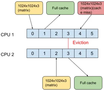
An example of cache contention is displayed in figure 4 explained as following: CPU no.1 loads data which partially or fully fills the 6MB cache and begins executing its task at time-stamp 0. Some point forward in time, CPU no. 2 loads also loads data which fills the cache, which according the the LRU policy evicts the data loaded by CPU no. 1. This happens at stamp 3. At time-stamp 4, CPU no. 1 tries and access data it previously loaded in, however this causes a cache miss. This leads to the data being loaded again for CPU no. 1.

(13)

Figure 4: Example of memory contention.

5 Research Questions

This study will investigate two research questions:

• Research Question 1: How can we use the knowledge of the execution characteristics of an algorithm to create adequately sized cache partitions?

• Research Question 2: Cache thrashing is very dependent upon the workload size. How can we determine sweet spots where cache partitioning is worth using?

6 Environment setup

The upcoming sections detail the different components used in our development and testing envi-ronment. As complement to the textual description in the upcoming sections, see appendix B for expected output from commands, especially when configuring Palloc.

6.1 Custom Linux kernel

In order to support palloc, we used kernel version 4.4.128. Palloc supports as late as Linux kernel version 4.4.X, therefore we chose to use Linux Kernel version 4.4.128. In terms of what makes the kernel custom, an additional flag was set, CONFIG CGROUP PALLOC = y, which includes Palloc as a kernel feature when compiling a new kernel.

For benchmarking, we have used a test which executes a cache demanding feature-detection algorithm called Speeded Up Robust Features (SURF). The test uses a number of images, which all load the cache differently.

(14)

To collect performance data about running processes, we use the performance counter API, PAPI.

6.2 Palloc configuration

We have configured Palloc to partition 8 of the 12 set bits of the cache. This is done by specifying the cache set bits in a mask, shown in figure 6, which is forwarded to the Palloc module. In our test system 64-bit addressing is used and a memory address is divided as shown in figure 5.

Figure 5: Composition of 64-bit memory address in our test system.

Since Palloc does not support automated calculation of cache set indexing bits, these have to be calculated by hand. Bits needed to be set for the mask in order to partition cache, varies depending on the memory address composition associated with the relevant architecture. The mask forwarded to Palloc is shown in figure 6.

Figure 6: The cache set index bits forwarded to Palloc illustrated and the mask in hexadecimal representation.

These are the steps to configure Palloc to use cache partitioning: 1. Set the mask in Palloc.

2. Create a new partition in the Palloc and Cpuset folders. Creating directories at the specified location will generate new partition hierarchies.

3. Set the number of bins that the new partition will use.

4. Set the cores and memory nodes the partition will use in Cpuset.

5. Either set PIDs for the partition or set all tasks running from the current shell to use the partition.

(15)

6. Finally, enable palloc.

The above steps explains how to setup a partition with Palloc. If more partitions are desired, all steps except step 1 and 6 need to be repeated. More detailed instructions are included in appendix A.

7 Method

To answer RQ1 we have recorded performance characteristics of executing processes, by recording LLC cache misses of executing processes, which are measured by the performance API (PAPI) [18]. We use PAPI in our controller to monitor LLC cache misses associated with priority processes. The recorded cache misses are used to determine cache partition sizes dynamically. A detailed description of the controller is specified in the next subsection.

The tool we have chosen to use for partitioning cache memory is a kernel level memory allocator, Palloc [14]. While Palloc originally is intended for DRAM bank partitioning, it has documented ability to partition cache memory combined with DRAM bank partitioning.

To answer research question 2 we intend analyze generated results from all our test, in order to try find sweet-spots for when cache partitioning is beneficial.

7.1 Prioritized cache partitioner

In our effort of answering research question 1 we have implemented a cache partition controller based on Palloc. Our implementation relies on Palloc in order to generate partitions of shared cache memory, assign generated partitions to different processes and cores and finally, repartition existing partitions dynamically during runtime. The cache partition controller is split into two different components, an initialization script and a C++ program.

7.1.1 Initialization Script

Before the controller can be used, Palloc needs to be configured. The initialization script edits the cpuset.cpus and cpuset.mems files in each generated partition directory under the /sys/fs/c-group/cpuset hierarchy. This enables partitions to use and be restricted to select CPUs/Cores and memory nodes. In other words, the values set in the cpuset.cpus and cpuset.mems files corresponds to allowed cores and memory nodes, e.g. 0 in cpuset.cpus assigns core 0 to that partition. Assign-ing these values are required parameters for Palloc, since Palloc relies on CGROUP for resource partitioning. While the script is treated as an separate entity in relation to the controller, it is invoked by the cache partition controller.

7.1.2 Cache partition controller

Our proposed cache partition sizing controller is mainly implemented in form of an user-space program. Once the controller has been executed, it continues to run until aborted by the user or the system. The main features of the controller is its ability to distribute processes to one of two segments based of their niceness priority. The segments are made up out of bins, where one bin corresponds to a partition of cache memory of 4KB.

Segment 1 is composed of 192 bins and is the prioritized segment. The segment controls tasks which has a niceness priority of 0 or less. All processes allocated to the prioritized segment will posses their own partition. The size of a partition is proportional to the percentage of L3 cache misses caused by an assigned process. The percentage corresponds to the fraction of the total L3 cache misses caused by all processes assigned to the priority segment.

Segment 2 is the un-prioritized segment, processes with a niceness priority higher than 0 will be allocated to this segment. Processes assigned to the un-prioritized segment competes for the 192-255 bin range.

(16)

Figure 7: Flowchart of partition controller for processing parsed process information. Given the flowchart in figure 7 of the controller, upon start-up the controller will fetch process information using the Linux command ”top”. The upper 10 processes are picked and their Process-ID(pid); Niceness(NI) and command(cmd) are parsed. Parsed information is stored in a data structure which programmatically represents a process in the controller.

After the controller has parsed collected process information, it will check the niceness value of each stored process. Based of the heuristics detailed earlier, processes are assigned to the prioritized and un-prioritized segments.

To calculate the bin ranges for prioritized processes, the controller uses cache misses. For each stored process the controller dispatches a thread running a monitoring program, which records the number of L3 cache misses associated with a relevant process through the PAPI interface.

We have used a sampling frequency of 2 seconds, after which all monitoring threads are syn-chronized and all recorded cache misses are summarized. The sum of all L3 cache misses is used to determine what percentage(P) of all cache misses each monitored process has caused in relation to the sum(CacheSum). The idea behind finding out the percentage of caused cache misses is that a process will be given a partition size proportional to the number of L3 cache misses it is associated with. The percentage of cache misses is the determining factor, which can be seen in equation (1), regarding what bin range size(RangeSize) a process will be assigned. For example, the total number bins is 128, if a process has contribution-percentage of 10 percent in relation to the cache miss sum. This would give the process a bin range size equivalent to 10 percent of 128 bins, rounded downwards to nearest integer.

RangeSize = CacheSum × P (2)

(17)

8 Limitations

We have done measurements on Linux kernel version 4.4.123, and implementations, investigations and measurements have been on a single specified architecture, detailed in table 2. More limitations concerning measurements is that we have used the feature detection algorithms from OpenCV version 2.4.13.6.

CPU Model Intel core i5 2540M Bit support 64-bit

L1 Cache size 32KB L1 Cache set assoc. 8-way L2 Cache size 256KB L2 Cache set assoc. 8-way

L3 Cache size 3MB L3 cache set assoc. 12-way

Cache line size 64B Executing CPUS 2 Number of Threads 4

Main memory size 8GB

Table 2: Hardware specifications of our test system.

9 Experiments

To answer our research questions we have created two experiments. The first experiment serves two purposes. Experiment 1 verifies if process isolation occur and if static partitioning increases execution time stability. Experiment 2 investigate if static partitioning can increase process stabil-ity. Experiment 2 also evaluates our cache partition controller, to investigate if it provides better process stability compared to static fair cache partitioning.

The experiments use an OpenCV test and a Leech. The OpenCV test runs all OpenCV SURF[19] on differently sized images displayed in table 3. Due to the different image sizes, the cache is loaded differently with each image. The Leech is a program which generates an artificial workload targeting the cache memory only at high speeds.

Image nr. Image Size Mem. Req. 1 103x103 32KB 2 209x209 131KB 3 295x295 262KB 4 591x591 1MB 5 1431x1431 6.1MB 6 2862x2862 24.6MB

(18)

9.1 Isolation experiment

The first experiment consists of 5 test cases and the purpose of the experiment is to investigate if process isolation can be increased with static cache partition sizes. Each test case uses static cache partition sizes in different setups. The first test case runs an OpenCV instance and a Leech in two different partitions with equal partition sizes. The second test case runs an OpenCV instance in a partition of 256 bins, and a Leech unpartitioned. Third test case runs an OpenCV instance in a partition of 255 bins, while a Leech runs in another partition using 1 bin. Fourth test case runs both an OpenCV instance and a Leech unpartitioned. Finally, in the fifth test case an OpenCV instance and a Leech are running in the same partition of 256 bins. More detailed instructions related to experiment 1 are included in appendix B.

Test case 1

Test case 1 runs an instance of the OpenCV test alongside a Leech instance. Both in equally sized partitions, each partition possesses half of the maximum number of bins. The OpenCV instance and the Leech will be running on different cores. Since we want to investigate if equally sized static partitions increase process isolation.

Steps for setting up and running test case 1 are as follows: 1. Create two partitions, call these part1 and part2. 2. Set memory node 0 to both partitions.

3. Set core 0 to part1 and core 1 to part2.

4. Set part1 bin range to first half of bins, and set the other half to part2. 5. Enable Palloc.

6. Start the OpenCV instance and assign its PID to part1.

7. Start the Leech instance after 100 iterations and assign its PID to part2.

8. Wait until the OpenCV test has done 500 iterations(is counted during runtime), after that kill both the OpenCV test and the Leech.

Test case 2

In test case number 2, an instance of the OpenCV test executes alone in a partition alongside an unpartitioned instance of the Leech. The aim of this test case is to further gather evidence that process isolation occurs, even if the Leech is running unpartitioned.

Steps on setting up and running test case 2 are as follows: 1. Create one partition and call it part1.

2. Assign memory node 0 and core 0 to part1. 3. Set number of bins for part1 to 256 bins. 4. Enable Palloc.

6. Start the Leech instance after 100 iterations of the OpenCV test has been performed. 7. Wait until the OpenCV test has done 500 iterations(is counted during runtime), after that

(19)

Test case 3

In test case number 3, an instance of the OpenCV test is run in a partition of 255 bins. Alongside it a Leech is inserted, which runs in another partition of 1 bin. The purpose of test case 3 is to investigate if process isolation is still increased when a second partition has 1 bin.

Steps on setting up and running test case 3 are as follows: 1. Create two partitions, part1 and part2.

2. Assign memory node 0 to both partitions. 3. Set 255 bins to part1 and 1 bin to part2. 4. Enable Palloc.

5. Start the OpenCV instance and assign its PID part1.

6. Start the Leech instance after 100 iterations and assign its PID part2.

Test case 4

Test case 4 involves running an instance of the OpenCV test and a Leech. Both the OpenCV test and the Leech executes unpartitioned. The purpose of this test case is to gather data that can be used to compare unpartitioned with partitioned performance.

Steps on setting up and running test case 4 are as follows: 1. Start the OpenCV instance.

2. Start the Leech instance after 100 iterations of OpenCV test has been done.

Test case 5

Test case number 5 is done to investigate how process execution time is affected when two processes compete in the same partition. The main difference between this test and test case 4 is the size of the memory. Test case 4 uses the entire cache while the size of the partition in test case 5 is equal to 256 bins. The purpose of this test is to collect fair data for the comparison while as mentioned before, test case 4 uses the entire L3 cache. This test involves running an instance of the OpenCV test alongside a Leech which is inserted at iteration 100, both are assigned to same partition.

Steps for setting up test case 5 as follows: 1. Create one partition and call it part1.

2. Assign memory node 0 and cores 0 and 1 to part1. 3. Assign 256 bins to part1.

4. Enable Palloc.

6. Start the Leech instance after 100 iterations and assign its PID to part1.

(20)

9.2 Prioritized controller experiment

The second experiment consists of two test cases and both test cases uses two identical OpenCV instances. In test case 1 two statically sized partitions are used, both using half of the maximum number of bins. Each partition is assigned an OpenCV instance. Test case 2 involves our controller, which dynamically resizes two partitions based of cache misses caused by respective OpenCV instance. More detail experiment instructions are included in appendix C.

Test case no. 1

Test case 1 uses two static partitions with equal amount of bins. Two identical OpenCV instances are used, each assigned to their own partition. Both OpenCV instances are executed at same time. The maximum number of bins in this test case is 192 bins, as this is the number of bins used by our controller for prioritized tasks.

Steps included in setup and performing this test case: 1. Create 2 partitions, part1 and part2.

2. Assign memory node 0 and core 0 to part1. 3. Assign memory node 0 and core 1 to part2. 4. Assign 96 bins to part1 and 96 bins to part2.

5. Start the OpenCV instances, assign PID of instance 1 to part1 and PID of instance 2 to part2.

6. Enable Palloc.

7. Wait until the OpenCV tests has done 500 iterations(is counted during runtime), after that kill both the OpenCV instances.

Test case no. 2

Test case 2 focuses on our cache partitioning controller. The cache partitioning controller sets the cache partition sizes of the two OpenCV instances.

Steps for running two process using the controller are as follow: 1. Execute the controller.

2. Start the two OpenCV instances simultaneous.

10 Results

Results presented in this section are data gathered when experiment 1 and 2 were performed. This chapter is structured as following: 10.1 presents the execution times recorded during experiment 1. 10.2 presents execution times recorded during experiment 2.

10.1 Experiment 1: Process isolation

Experiment 1 consists of 5 test cases. Each test case runs an instance of OpenCV SURF and a Leech that targets cache memory. The data we gathered is the execution times achieved by the OpenCV instance when it is provided different sized images. Test case 1 runs OpenCV SURF and a Leech in two different equally sized partitions. Test case 2 runs OpenCV SURF in a partition of 256 bins and a Leech unpartitioned. Test case 3 runs OpenCV SURF in a partition of 255 bins and Leech in a partition of 1 bin. Test case 4 runs OpenCV SURF and a Leech unpartitioned. Finally, test case 5 runs OpenCV SURF and a Leech in the same partition of 256 bins.

(21)

Test case 1

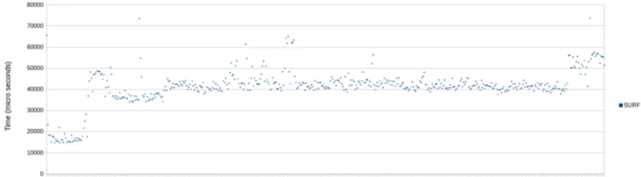
Test case 1 runs an OpenCV instance with a Leech, which inserted at iteration 100. Each program is assigned to two different equally sized (128 bins each) partitions. The test case is repeated 4 times, each time with a different sized image provided to the OpenCV instance. Gathered results are presented in figures 8 to 11.

Figure 8: Recorded execution times of OpenCV surface detection algorithFm using 262KB image. Running in a partition with half of max bins, with leech inserted at iteration 100 in a partition of other half of max bins.

Figure 9: Recorded execution times of OpenCV surface detection algorithm using 1MB image. Running in a partition with half of max bins, with leech inserted at iteration 100 in a partition of other half of max bins.

(22)

Figure 10: Recorded execution times of OpenCV surface detection algorithm using 6.1MB image. Running in a partition with half of max bins, with leech inserted at iteration 100 in a partition of other half of max bins.

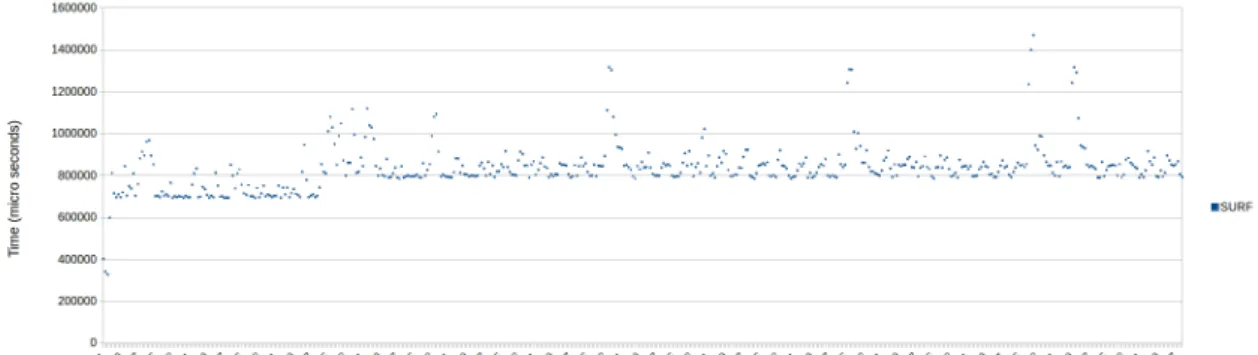
Figure 11: Recorded execution times of OpenCV surface detection algorithm using 24.6MB image. Running in a partition with half of max bins, with leech inserted at iteration 100 in a partition of other half of max bins.

We observe that stability in the OpenCV instance varies between the different images sizes. Figure 8 shows instability at the beginning of test, but becomes stable towards the end of test. Figure 9 has more even stability compared to figure 8, since execution times are not as sporadic during the first 100 iterations compared to figure 8. In figure 10 we see spikes in the execution time, starting from around iteration 240. Similar spikes also occur in figure 11, but at a more dense frequency compared to what is seen in figure 10. Another shared pattern seen in figures 10 and 11 is that both are stable before the Leech insertion point. Finally, a shared effect seen in all figures, is the jump in execution time starting from the Leech insertion point.

Test case 2

Test case 2 runs an OpenCV instance in a partition of 256 bins and a Leech unpartitioned, which is inserted at iteration 100. Test case 2 is repeated 4 times with different sized images provided to the OpenCV instance each time. Results are presented in figures 12 to 15.

(23)

Figure 12: Recorded execution times of OpenCV surface detection algorithm using 262KB image. Running in a partition with max bins, With leech inserted at iteration 100 unpartitioned.

Figure 13: Recorded execution times of OpenCV surface detection algorithm using 1MB image. Running in a partition with max bins, With leech inserted at iteration 100 unpartitioned.

Figure 14: Recorded execution times of OpenCV surface detection algorithm using 6.1MB image. Running in a partition with max bins, With leech inserted at iteration 100 unpartitioned.

(24)

Figure 15: Recorded execution times of OpenCV surface detection algorithm using 24.6MB image. Running in a partition with max bins, With leech inserted at iteration 100 unpartitioned.

Figure 12 shows instability in the beginning of the test, but becomes gradually more stable towards the end of test. Figure 9 shows more stability compared to figure 12, also the pattern here is that stability increases over time. While figure 10 shows that execution time is stable even after the Leech insertion point, we observe reoccurring spikes in the execution time, similarly to figure 10. The same is seen in figure 15 where spikes occur at a more dense frequency, stability is also worse in figure 15 compared to figures 13 and 14.

Test case 3

Test case 3 uses two partitions, one partition with 255 bins and another with 1 bin. An OpenCV instance is assigned to the partition with 255 bins and a Leech to the partition with 1 bin. The leech is inserted at iteration 100 and the test case is repeated 4 times. Each time a different sized image is provided to the OpenCV instance. Results are presented in figures 16 to 19.

Figure 16: Recorded execution times of OpenCV surface detection algorithm using 262KB image. Running in a partition with 255 bins, With leech inserted at iteration 100 in a partition of 1 bin

(25)

Figure 17: Recorded execution times of OpenCV surface detection algorithm using 1MB image. Running in a partition with 255 bins, With leech inserted at iteration 100 in a partition of 1 bin

Figure 18: Recorded execution times of OpenCV surface detection algorithm using 6.1MB image. Running in a partition with 255 bins, With leech inserted at iteration 100 in a partition of 1 bin

Figure 19: Recorded execution times of OpenCV surface detection algorithm using 24.6MB image. Running in a partition with 255 bins, With leech inserted at iteration 100 in a partition of 1 bin

(26)

The results presented in figure 16 shows that execution time stability is lacking. Since execution times are sporadic and differ substantially from iteration to iteration. Figure 17 on the contrary shows more stability than what is seen in figure 16. Similarly to what we saw in test cases 1 and 2 when the 1MB and the 6.1MB images are used, spikes in execution occurs which can be observed in figures 17 and 18. Similar to test case 1 and 2, spikes occur more at a more dense frequency when the 6.1MB is used, presented in figure 18. Finally, in figure 19 stability is affected by the Leech more compared to 8, 17 and 18. We can also see spikes in the execution time pattern in 19 at even more dense frequency compared to figure 18.

Test case 4

Compared to test cases 1 to 3, test number 4 is different. The main difference is that OpenCV instances and Leech runs unpartitioned. The same as the other tests, Leech insertions is at iteration 100 and it is noticeable in the presented graphs.

Figure 20: Recorded execution times of OpenCV surface detection algorithm using 262KB image unpartitioned, with leech inserted at iteration 100 unpartitioned.

Figure 21: Recorded execution times of OpenCV surface detection algorithm using 1MB image unpartitioned, with leech inserted at iteration 100 unpartitioned.

(27)

Figure 22: Recorded execution times of OpenCV surface detection algorithm using 6.1MB image unpartitioned, with leech inserted at iteration 100 unpartitioned.

Figure 23: Recorded execution times of OpenCV surface detection algorithm using 24.6MB image unpartitioned, with leech inserted at iteration 100 unpartitioned.

Results from test 4 are presented in figures 20 to 23. Since in test 4, both OpenCV instance and Leech executes unpartitioned, the spike of the Leech insertion is noticeable in all graphs at iteration 100. Before starting Leech, the execution time of the OpenCV instance remains stable. However, at iteration 100 after Leech insertion, the execution time becomes less stable.

Test case 5

Test case 5 uses a partition of 256 bins. Both an instance of the OpenCV test and a Leech inserted at iteration 100 are assigned to the same partition. The test case is repeated 4 times, each time with a different sized image provided to the OpenCV instance. Results are presented in figures 24 to 27.

(28)

Figure 24: Recorded execution times of OpenCV surface detection algorithm using 262KB image with leech inserted at iteration 100, both assigned to same partition of 256 bins.

Figure 25: Recorded execution times of OpenCV surface detection algorithm using 1MB image with leech inserted at iteration 100, both assigned to same partition of 256 bins.

Figure 26: Recorded execution times of OpenCV surface detection algorithm using 6.1MB image with leech inserted at iteration 100, both assigned to same partition of 256 bins.

(29)

Figure 27: Recorded execution times of OpenCV surface detection algorithm using 24.6MB image with leech inserted at iteration 100, both assigned to same partition of 256 bins.

We can see in figures 24 to 27 that execution time is unstable, which is similar to what we saw in figures 20 to 23. Spikes in execution is also seen at iteration 100, when the Leech is inserted. However, we see that figures 24 to 27 presents worse stability compared to figures 20 to 23. Summary experiment 1

From the results gathered in experiment 1 we can see that images of 262KB and larger cause spikes in execution time across all test cases. Test cases 4 and 5 presented similar results, while test case 5 showing worse stability than test case 4.

10.2 Experiment 2: Prioritized partition controller

Following data are gathered from test cases where fair static cache partition sizing and our con-troller are used. The layout of the graphs is the following: a graph associated with a given image size related to fair static partition sizing, is always followed by a graph related to our controller using same image size. This layout provides an observable contrast between the two different par-tition sizing approaches.

Test case 1 runs two instances of OpenCV SURF in parallel on different cores with the same image size each time. Each OpenCV test is assigned to a separate partition of 92 bins respectively. Test case 2 runs two instances of OpenCV in parallel on different cores using the same image size each time. Each instance is assigned to a separate partition, which sizes are adjusted by our controller, that determines sizes based on caused cache misses of respective instance.

Figure 28: Execution times of two OpenCV test processes using 32KB image, running in static equally sized partitions. Each partition is 96 bins.

(30)

Figure 29: Execution times of two OpenCV test processes using 32KB image, running in dynami-cally sized partitions, proportional to caused cache misses.

Figure 31: Execution times of two OpenCV test processes using 131KB image, running in dynam-ically sized partitions, proportional to caused cache misses.

(31)

Figure 33: Execution times of two OpenCV test processes using 262KB image, running in dynam-ically sized partitions, proportional to caused cache misses.

Figure 34: Execution times of two OpenCV test processes using 1MB image, running in static equally sized partitions. Each partition is 96 bins.

(32)

Figure 35: Execution times of two OpenCV test processes using 1MB image, running in dynamically sized partitions, proportional to caused cache misses.

Figure 36: Execution times of two OpenCV test processes using 6.1MB image, running in static equally sized partitions. Each partition is 96 bins.

Figure 37: Execution times of two OpenCV test processes using 6.1MB image, running in dynam-ically sized partitions, proportional to caused cache misses.

(33)

From the presented results of experiment 2 we can see when the 32KB, 131KB, 1MB and 6.1MB images are used, fair static partition sizing does not have the upper hand on our controller. When these three images are used, our controller provides better stability compared to fair static partition sizing, which can be seen when comparing figure 28 with 29; figure 30 with 31; figure 34 with 35 and figure 36 with 37. The exception is when the 262KB image, figure 32 and 33, is used. In this case, fair static partition sizing outperforms our controller. However, in figures 34, 35, 36 and 37 we can see deviations in the execution pattern, recognizable as spikes in respective figures. The spikes are recorded both when fair static partition sizing and when our controller is used. Another pattern breaking occurrence can be observed in figures 29 and 31, where SURF process 2 shows better stability than the other. Both these instances are observed when our controller is used.

(34)

11 Discussion

The execution times presented in figures 24-27 are unstable, we think this is most likely due to inter-process interference. Since the OpenCV instance and the Leech are unpartitioned, we conclude they are not isolated from each other. However, an important aspect of results presented in figures 20-23 is results have been gathered when the entire L3 cache has been used. Since the entire L3 cache has been used, figures 20-23 alone are not sufficient enough to draw a solid conclusion from. For this reason we performed test case 5, results are presented in figures 24-27. Test case 5 is formulated almost identically to test case 4. The difference is the partition configuration, in test case 5 the OpenCV instance and the Leech are assigned to the same partition of 256 bins. Given the partition size, results in figures 24-27 becomes more relevant and comparable to results from test cases 1, 2 and 3. The conclusion we can draw from figures 20-23 and 24-27 is that they show similar behaviors. Despite the fact they are using different amounts of cache memory. We interpret this as an indication of process interference and is good to use as a comparative base.

Taken into account figures 20-23 and 24-27 we have a basis which shows how execution time behaves in a non-isolated system. To investigate if process isolation increases with static cache partition sizes, we conducted test cases 1, 2 and 3. We start comparing figures 24-27 with 24-27 and we see a difference in execution time stability between them. Figures 24-27 show more stable execution time and from this we can draw a conclusion about fair and equal partition sizes. It in fact increases stability thanks to the additional isolation which occurs as result of static cache partition sizes. Had this not been the case, the opposite would be more logical where figures 8-11 did not show an increase in reliability.

We can see unexplained anomalies regarding stability in figure 10. The same anomalies occurs in figures 18, 22 and 26. We assume these anomalies are not associated with the partition sizes or process isolation. Instead we speculate, the cause is likely related to image 3 in some manner. We also speculate it could be kernel interrupts which might be the cause, but since the common denominator is image 3, we think it is far-fetched.

Another anomaly can be observed in figure 16. When we compare figure 16 to figures 8, 20 and 24, the result in figure 16 is different. The stability is considerably lower compared to what can be seen in figures 8, 20 and 24, which all where conducted using the same sized image as figure 16. However, figure 16 seems to be similar to figure 24, where the OpenCV instance and a Leech shares the same partition. The cause of this anomaly is difficult to determine and we speculate it could be the human factor which is responsible. However, we do not accept this cause entirely since the system could also be responsible as well.

Conclusively regarding results from experiment 1, we find a general conclusion can be drawn that process isolation has been increased with static cache partition sizes. Despite observed anoma-lies, we still find the evidence is enough in favor of increased process isolation and reliability. Finally, from experiment 1 we also find fair static cache partition sizes to be useful regardless of what image size we used. With exception for image number 3 which is not benefiting from static fair cache partition sizes, for an unknown reason.

The results from experiment 2, where we compared the stability of fair static partition sizing with our controller. Starting with the static approach, we see results presented in figures 28, 30, 32, 34 and 36 has good stability. However, figures 30 compared to 30, 32, 34 and 36 shows lower stability. We argue the cause could be related to the image sizes, since the same is recorded when our controller is used in figure 31. Another oddity we find is one process in figures 28, 29, 30, 31, 32 and 33 outperform the other process in terms of stability. This behavior can be explained as kernel related, since the system is still running processes in the background and could be using the same core as the more unfortunate process. This reason could be what is happening and it would explain why only one process is affected since each process runs on a separate core. However, the execution time stability is more equal between the processes when our controller is used.

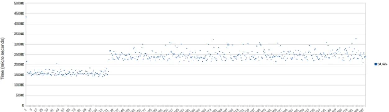
We compare the results on an image-by-image basis, starting with image 1. In this case our controller has the upper hand on the static approach. Our controller yields a better stability at the cost of longer execution time, which is to be expected given the fewer cache resources available.

Moving on to image 2, here our controller gains the upper hand, but with smaller marginal compared to image 1. We find our controller delivers higher stability but also suffers from uneven

(35)

core stability. There is also an anomaly where the execution time jumps significantly, this is most likely due to bad repartitioning, e.g. 0 cache misses might have been recorded. Since red process is more stable compared to blue process in figure 31, red process might have been given a larger amount of bins.

Image 3 is the case where our controller does not perform better than the static approach. Figures 32 and 33 compared, shows the static partition sizes deliver a better stability. We try to find a logical cause to this behavior, but we can not formulate an explanation for it. We speculate the cause is not related to the partition sizing approaches, as the behavior is observed in both static partition sizes and with our controller. However, more detailed investigation is needed to fully determine the cause and we leave it for future work.

With image 4 our controller is performing better than static partition sizes, but not with a big marginal. An oddity we find with image 4 is sudden spikes in execution times occurs. Since spikes occurs both with static partition sizes and our controller. We speculate the cause for these spikes is related to the image size.

Similarly to image 4, we find image 5 shows better stability with our controller which we can see when comparing figures 36 and 37. However, also with image 5 we can see spikes in the execution time. Spikes occurs in both approaches, which in our opinion is a sign the cause is not related to the partition sizing approaches. Instead we speculate the cause is associated with the image size, same as with image 4. The difference being the spikes occur in a more frequent pattern, compared to the spikes in figures 34 and 35.

Conclusively, regarding results gathered in experiment 2, we find our controller provides better stability during almost all of the OpenCV image tests. However, there are anomalies in the execution time, but we argue these anomalies are insignificant as the results are in majority in favor of our controller.

Given the interpretation on we have done on the results from experiment 1 and 2. We find our research questions to have been answered. Our first research question put focus on how adequate partition sizes can be determined using execution characteristics. Our interpretation of gathered results shows both unfair and fair static partition sizes can be used to size partitions and provide a better stability. Our interpretation also shows dynamically sizing partitions proves to be more beneficial then static in most cases.

Since we conducted tests with different sized input data to the OpenCV test, and we also used different partition sizing approaches. Collectively, results from experiment 1 and 2 shows dynamic cache partition sizing is worth using regardless to the input size used in our tests. Since dynamic cache partition sizing is worth using regardless to the input size, we find our second research question can not be answered. The main reason as we speculate is the limited amount of used test data. The reason behind our speculation is that we can not predict how the result would be effected if we used other sized test data.

However, the benefits of dynamic cache partition sizing are differing, we leave it up to situational determination whether cache partitioning is worth using for increased process reliability. Since cache partitioning leads to longer execution time so in the cases where execution time can be sacrificed for reliability, cache partitioning is a feasible option.

In relation to previous related work, we find our work is alone focusing on increasing process reliability. Other works have tried to increase system utilization and lower energy consumption. Other previous work have employed a mixture of static and dynamic cache partitioning on different cache levels. However, our work is alone focusing on shared LLC partitioning with special focus on the L3 cache. We also put heavy focus on the partition sizes, which other related works do not. Finally, we argue that we have not taken a general approach with our controller, since we have only taken into account a specific program/algorithm. The measurements are also specific to certain load sizes so we cannot say our results are generalizable. Finally, we find the anomalies in the results suggests there could be a need for complementing methods, if a higher process reliability is wanted.

(36)

12 Conclusions

In this work we investigated different cache partition sizes to try and find sweet spots for when cache partitioning is worth using. We also investigated if we can size cache partitions using execution characteristics of an algorithm. To fulfill these purposes we investigated unfair and fair static cache-coloring based cache partition sizes. We also investigated effects of dynamic cache-coloring based cache partitioning with cache misses as partitioning sizing heuristic.

Our results shows fair and unfair static cache partition sizes increases process reliability at the cost of execution time. We find that if the sacrifice of higher execution time can be made, static partition sizing is an option to be considered if higher reliability is wanted. Our results also shows dynamic cache partition sizing outperforms fair static partition sizing in all expect one of our test cases. This suggests cache misses are a feasible execution characteristic that can be used to determine cache partition sizes dynamically. The downside of both the static and the dynamic approaches is their cost in execution time due to lesser available resources. We also found our controller might be too resource demanding to be used in older architectures as frequent memory crashes occurred, when we ran memory heavy tests.

Our test results includes anomalies in execution time stability, which suggests cache partitioning alone might not be enough to ensure high process reliability. But we concluded that most of these anomalies to be of external sort, and not directly associated with partition sizing methods. We also could not explain certain anomalies as they required more in-depth investigation. Suggestively, cache partitioning needs to be complemented with other process reliability increasing methods. This would guarantee higher process reliability.

While our test results show cache partitioning is beneficial in many cases, the results are no way a general conclusion. Since our measurements were conducted on very specific data loads.

13 Future Work

For the future we think our work can be extended in multiple ways. Since our experiment include a limited data span, more input data could be added to give more metrics. The additional metrical data could contribute to a more generalizable and more detailed result.

We also think future work can be done to investigate the unanswered anomalies recorded in our results. Since we could not give concrete answers to why certain anomalies occurred, these can be further analyzed and answered.

A possible extension to our work could be to involve a different partition sizing heuristic. An example is to sample how much cache memory processes use, then size partitions proportional to cache memory usage. This example could also be combined with cache misses for more fine-tuned and specific partition sizes.

Another future extension can be usage of a more powerful test system. A more powerful test system would allow more intensive experiments. This could show how our controller behaves in a different system which may have more cores and/or larger caches. Finally, the same extension can be used to investigate behavior in a heavily loaded system.

(37)

References

[1] D. A. Patterson and J. L. Hennessy, Computer organization and design, T. Green and N. Mc-Fadden, Eds. Morgan Kaufmann Publishers, 2012.

[2] R. Karedla, J. S. Love, and B. G. Wherry, “Caching strategies to improve disk system perfor-mance,” Computer, vol. 27, no. 3, pp. 38–46, March 1994.

[3] T. King, “Managing cache partitioning in multicore processors for certifiable, safety-critical avionics software applications,” in 2014 IEEE/AIAA 33rd Digital Avionics Systems Confer-ence (DASC), Oct 2014, pp. 8C3–1–8C3–7.

[4] C. Xu, X. Chen, R. P. Dick, and Z. M. Mao, “Cache contention and application performance prediction for multi-core systems,” in 2010 IEEE International Symposium on Performance Analysis of Systems Software (ISPASS), March 2010, pp. 76–86.

[5] H. Al-Zoubi, A. Milenkovic, and M. Milenkovic, “Performance evaluation of cache replacement policies for the spec cpu2000 benchmark suite,” in Proceedings of the 42Nd Annual Southeast Regional Conference, ser. ACM-SE 42. New York, NY, USA: ACM, 2004, pp. 267–272. [Online]. Available: http://doi.acm.org/10.1145/986537.986601

[6] T. King, “Managing cache partitioning in multicore processors for certifiable, safety-critical avionics software applications,” in 2014 IEEE/AIAA 33rd Digital Avionics Systems Confer-ence (DASC), Oct 2014, pp. 8C3–1–8C3–7.

[7] M. Shekhar, A. Sarkar, H. Ramaprasad, and F. Mueller, “Semi-partitioned hard-real-time scheduling under locked cache migration in multicore systems,” in 2012 24th Euromicro Con-ference on Real-Time Systems, July 2012, pp. 331–340.

[8] K. Nikas, M. Horsnell, and J. Garside, “An adaptive bloom filter cache partitioning scheme for multicore architectures,” in 2008 International Conference on Embedded Computer Systems: Architectures, Modeling, and Simulation, July 2008, pp. 25–32.

[9] J. Lin, Q. Lu, X. Ding, Z. Zhang, X. Zhang, and P. Sadayappan, “Gaining insights into multicore cache partitioning: Bridging the gap between simulation and real systems,” in 2008 IEEE 14th International Symposium on High Performance Computer Architecture, Feb 2008, pp. 367–378.

[10] N. Suzuki, H. Kim, D. d. Niz, B. Andersson, L. Wrage, M. Klein, and R. Rajkumar, “Coordi-nated bank and cache coloring for temporal protection of memory accesses,” in 2013 IEEE 16th International Conference on Computational Science and Engineering, Dec 2013, pp. 685–692. [11] Y. Ye, R. West, Z. Cheng, and Y. Li, “Coloris: A dynamic cache partitioning system using page coloring,” in Proceedings of the 23rd International Conference on Parallel Architectures and Compilation, ser. PACT ’14. New York, NY, USA: ACM, 2014, pp. 381–392. [Online]. Available: http://doi.acm.org/10.1145/2628071.2628104

[12] (2018) cgroups - linux control groups. [Online]. Available:http://man7.org/linux/man-pages/ man7/cgroups.7.html

[13] (2012) numa - overview of non-uniform memory architecture. [Online]. Available: http://man7.org/linux/man-pages/man7/numa.7.html

[14] H. Yun, R. Mancuso, Z. P. Wu, and R. Pellizzoni, “Palloc: Dram bank-aware memory allo-cator for performance isolation on multicore platforms,” in 2014 IEEE 19th Real-Time and Embedded Technology and Applications Symposium (RTAS), April 2014, pp. 155–166. [15] X. Zhang, S. Dwarkadas, and K. Shen, “Towards practical page coloring-based multicore

cache management,” in Proceedings of the 4th ACM European Conference on Computer Systems, ser. EuroSys ’09. New York, NY, USA: ACM, 2009, pp. 89–102. [Online]. Available: http://doi.acm.org/10.1145/1519065.1519076

CONTROLLING CACHE PARTITIONSIZES TO INCREASE APPLICATIONRELIABILITY

V¨

aster˚

as, Sweden

Undergraduate Thesis

CONTROLLING CACHE PARTITION

SIZES TO INCREASE APPLICATION

RELIABILITY

Janne Suuronen

jsn15011@student.mdh.se

Jawid Nasiri

jni15001@student.mdh.se

Examiner: Masoud Daneshtalab

Supervisor: Jakob Danielsson

Contents

1

Introduction

2

Background

2.1

Symmetrical Multi-processors

2.2

Cache hierarchies in SMP

2.3

Cache misses and cache contention

2.4

Least Recently Used Policy

2.5

Cache-Partitioning

2.6

Cache-Coloring

2.7

Cgroups - Linux control groups

3

Related Work

3.1

COLORIS

3.2

PALLOC: DRAM Bank-Aware Memory Allocator for Performance

Isolation on Multicore Platforms

3.3

Towards Practical Page Coloring-based Multi-core Cache

Manage-ment

3.4

Dynamic Cache Reconfiguration and Partitioning for Energy

Opti-mization in Real-Time Multi-Core Systems

3.5

Time-predictable multicore cache architectures

3.6

Semi-Partitioned Hard-Real-Time Scheduling Under Locked Cache

Migration in Multicore Systems

4

Problem Formulation

5

Research Questions

6

Environment setup

6.1

Custom Linux kernel

6.2

Palloc configuration

7

Method

7.1

Prioritized cache partitioner

8

Limitations

9

Experiments

9.1

Isolation experiment

9.2

Prioritized controller experiment

10

Results

10.1

Experiment 1: Process isolation

10.2

Experiment 2: Prioritized partition controller

11