Income Growth and Income Inequality in Danish Municipalities

0 BACHELOR THESIS

THESIS WITHIN: Economics NUMBER OF CREDITS: 15hp

PROGRAMME OF STUDY: International Economics and Policy AUTHOR: Mattias Lindell

SUPERVISOR: Michael Olsson JÖNKÖPING December, 2017

Income Growth and Income Inequality in

Danish Municipalities

BACHELOR THESIS WITHIN: Economics NUMBER OF CREDITS: 15 ECTS

PROGRAMME OF STUDY: International Economics and Policy

AUTHOR: Mattias Lindell JÖNKÖPING December 2017

i

Bachelor Thesis in Economics

Title: Income Growth and Inequality in Danish Municipalities

Authors: Mattias Lindell Tutor: Michael Olsson Date: 2018-01-01

Income inequality, Gini coefficient, income growth, regional economics, Denmark

Abstract

Income growth and income inequality is an important theme in Economic research. It has been debated for decades whether income inequality hinders or enhances income growth. One of the classic models of this relationship was the Kuzenets curve which shows inequality against income per capita can be defined by an inverted U-shaped curve, over a period of time. The purpose of the paper is to see to see the relationship between income growth and inequality on a municipality level. To do this, four econometric panel data models were constructed with data gathered from Statbank Denmark. Log of income was used as the dependent variable and different measures of inequality were used as independent variables among other variables (public expenditure, education, population density, demographic composition, taxation). Results from these models show how income growth is positively related to income inequality, with vastly higher growth at the top end of the income distribution in Denmark. The

implications of these findings can show that a trade-off between income inequality and income growth is not true, and it is possible that both variables work in tandem. Other factors such as education and demographic composition were also positively correlated with income growth, while other factors, such as taxation, were statistically insignificant. Comprehensive research on inequality and income growth at a municipality level is sparse, especially in the case of

ii

Contents

I. Introduction ... 1

II. Previous Studies ... 3

A. Kuznets’s curve and Gini in Denmark ... 3

B. Income Inequality Insignificant or Hindrance to Growth ... 5

C. Income Inequality Insignificant or Benefit to Growth ... 6

D. Similar Regional Studies ... 7

III.

Data and Framework ... 9

A. Sample and remarks ... 9

B. Variables ... 10

C. Descriptive statistics ... 14

IV.

Methodology ... 17

A. Econometric Model ... 17

B. Endogeneity Issue ... 18

C. Tests for Model ... 19

V. Conclusions ... 22

A. Empirical Findings ... 22

B. Limitations and Possibilities for Further Research ... 30

VI.

References ... 32

VII. Appendix ... 34

A. Tables ... 34

1

I.

Introduction

In economics, the question whether income inequality hinders or enhances economic growth has been discussed in great detail for many decades. Income inequality refers to the disparity in income within a group or across a society; usually characterized by the aphorism ‘the rich get richer while the poor get poorer’. Income inequality in society has been said to be closely correlated with an increase in crime, where marginalized members of society are more likely to feel resentment due to their economic position or competition over sparse jobs increasing the propensity to commit crimes (Birdsong, 2015). There have also been links where poorer individuals often have limited access to healthy foods and healthcare facilities, rendering these groups more prone to disease, higher mortality rates, and being a less effective workforce. Education is also hampered in unequal economies where there is little incentive or little money viable to invest into garnering a proper education (Pickett and Wilkinson, 2017). Time is also better spent for lower income individuals working rather than studying.

As a result, income growth is of great importance since many of the challenges facing individuals with lower income could be alleviated with increases in income growth. Furthermore, it is important to assess which factors and variables are significant to better understand what forces may be behind a rise or fall in income inequality and/or whether this has a positive or negative impact on the economy.

There also exists detrimental effects to having a society where income inequality does not exist, i.e. there is perfect income distribution. In a society where all are making equal amounts no matter what occupation, effort or expertise there exists no incentive to work harder, obtain higher education since everyone would make the same income no matter what.

2

I intend to study and analyze the relationship between income growth and income inequality at the municipality level through (and inclusive of) the years 2008-2016, using several different measures of income inequality. This will be accomplished through the use of a growth-inequality model which tests if and how income growth-inequality affects income growth, depending on a set of control variables. The aim is to see whether Danish municipalities’ income growth is affected positively or negatively by income inequality and if this changes with different

measurements of income inequality. Following Voitchovksy (2005) and Cialani (2013) a growth model will be constructed that tests the relationship between income growth and the upper and lower ends of Denmark’s income distribution. Hopefully, this paper helps to improve knowledge of possible links and correlations between income inequality and income growth with the multiple explanatory variables used, on a smaller municipality scale, as plenty of research have already been done on national levels.

3

II. Previous Studies

A.

Kuznets’s curve and Gini in Denmark

One of the founding and most important works of literature Economic Growth and Income

Growth (Kuznets, 1955) concludes that inequality against income per capita can be defined by

an inverted U-shaped curve (Figure 1). As income per capita is initially starting to increase so does inequality up until a turning point, whereas income per capita is rising so inequality begins to fall. In other words, income inequality first rises in nations but begins to fall the more

developed said country becomes. Barro (2000) argued that income inequality where countries were already developed did lead to growth, but in poorer countries tended to deter growth. His data empirically shows the Kuznets growth did exist with regularity across his panel of countries which included Denmark. Historically many studies Paukert (1973), Papanek and Kyn (1986), Ram (1995), Tsakoglou (1988), to name a few, have all corroborated what Kuznets stated in research regarding development and growth. Yet during the past decade or so developed nations have seen the possible end of Kuznets curve as many developed nations are being to rise in income inequality, this next stage of development not foreseen by Kuznets. Gallup (2012) suggests that although evidence of the Kuznets curve may have existed for previous decades, current data shows a trend of developed nations rising in income inequality, thus leading to a U-shaped curve.

4

Figure 1: Kuznets’s Curve

A study conducted by OCED in 2011, states that from mid-1980 to the late 2000s only Turkey, Greece, France, Hungary, and Belgium out of all the OCED countries (Denmark being an OCED member nation) have experienced no increase or slight decreases in their Gini coefficients1_.

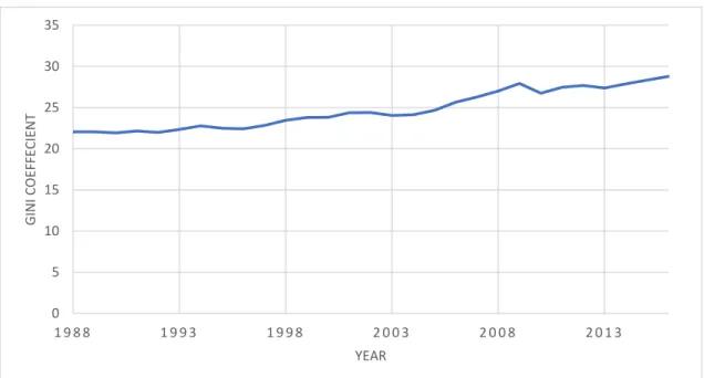
According to Cevea, a Danish thinktank, since 2002 the top one percent of Danish earners have seen their income rise by 30 percent while the poorest Danish have seen ten percent less income than they did in 2002. Figure 2 shows the steady Gini coefficient increase Denmark has seen from 1988 to 2016.

1 _{The Gini Coefficient is statistical measurement of income distribution. The coefficient ranges from 0 to 1, with 0}

meaning perfect equality and 1 being perfect inequality. For the purpose of this paper, the Danish Statbank decided to multiply the Gini coefficient by 100, meaning the new the range is 0 to 100.

5

Figure 2: Denmark Gini coefficient 1988-2016

B.

Income Inequality Insignificant or Hindrance to Growth

Research throughout the decades has been dedicated to studying whether or not income inequality hinders or stimulates economic growth. Regarding the case that low level of income inequality may have a positive effect on a country’s economic growth; this was shown in the case in East Asia (Birdsall, et al., 1995). Birdsall et al, found that during the last three decades East Asia has managed to keep relatively low levels of income inequality with unprecedented economic growth, as was the case with China, South Korea, Japan etc. A conclusion was that policies that promoted and expanded education also promoted economic growth.

Alesina and Rodrik (1994) found that high income inequality was a hindrance to economic growth. In a panel data sample of over 100 countries, Alesina and Rodrik concluded that with the greater the inequality of wealth and income the higher rate of taxation would be present, which led to slower economic growth. Aghion et al (1999) also find a negative relationship

0 5 10 15 20 25 30 35 1 9 8 8 1 9 9 3 1 9 9 8 2 0 0 3 2 0 0 8 2 0 1 3 G IN I CO EF FE CIE N T YEAR

6

between economic growth and income inequality in particular, when capital markets are imperfect and/or when agents suffer from institutional limitations in access to investment.

On the other side, research exists to show that wealth and income inequality may be unrelated to or have a positive effect on economic growth. Li and Zhou (1998), in a direct response to Alesina and Rodrik (1994) argued that income inequality has at most an ambiguous effect on economic growth and could theoretically have a positive effect. Li and Zhou found that in their panel data set covering 112 developed and developing nations over the years 1947-1994 had a positive relationship with economic growth with Gini as the inequality measure. Venture capitalist, entrepreneur Paul Graham (2016) argues that income inequality is a necessary evil and a positive influence on economic growth. Graham argues that some causes of income inequality are not a hindrance to the economy; for example, people who are creating

companies, jobs, and innovation, are increasing their income disproportionally to those who work for them but the benefits they are providing are too good to turn down.

C.

Income Inequality Insignificant or Benefit to Growth

Several arguments have been made to suggest a positive relationship between income growth and income inequality. One of these arguments is that inequality enriches growth through more expansive investment opportunities. This happens under the assumption that there are investments with large setup costs, and imperfections in the credit-market exist. With these parameters, a high amount of wealth would be needed to invest in these projects. With unequal wage distribution there are more people of high wealth available and ready to invest into these projects, as opposed when there are more equal wages (Aghion et al., 1999) (Barro, 2000). A secondary argument suggests that the individual’s savings rates increase with their personal wealth level. In this vein, if there is a redistribution of wealth from rich to poor the overall saving levels could decrease. This is especially the case for closed economies when savings rates are equal to domestic investments (Aghion et al., 1999). A final argument is that

7

equal wages would discourage workers from working to their fullest potential. Instead, a society where unequal wages exists would incentivize workers to exert more effort to achieve higher wages (Aghion et al., 1999). On the other hand, arguments exist to suggest that a negative relationship between income growth and inequality exists. A commonly presented argument is that more equalized wages reduce crime, corruption, and social unrest by

diminishing credit restraints, which allows for investment in human and physical capital (Alesina and Rodrik 1994; Aghion et al., 1999; Barro, 2000).

Other research papers argue that income inequality and economic growth can be positively and negatively related depending on the measure of inequality. Barro (2000) using a broad panel of countries shows that a negligible to a nonexistent relationship between income inequality, and rates of growth/ investments exist. In the case of poor countries though, there is evidence to show that inequality hinders growth while in richer regions inequality promotes growth. Growth tends to decline when GDP per capita is below $2000 and tend to increase when GDP per capita is above $2000. Another research paper in the same vein of Barro (2000) is that of Voitchovsky (2005). Voitchovsky uses panel data of 25 countries over a five-year period. Results from the paper suggest that the top end of income inequality is associated with an increase in growth, while bottom end income inequality is associated with a decrease in growth.

D.

Similar Regional Studies

To my knowledge, there exists no previous study on the relationship between income inequality and average income growth for Danish municipalities. Ioana Neamtu and Niels Westergaard-Nielsen (2013) in their report Sources and Impact of Rising Inequality in Denmark analyse the reasons and impacts for a nation with a growing income and income equality on a national level. Similar papers have been done on Swedish municipalities (Cialani, 2013), Swedish counties (Nahum, 2005), Swedish labour markets (Rooth and Stenberg, 2012) and Norwegian municipalities (Fjære, 2014).

8

The most similar report to this research paper is Cialani (2013) who conducted research on the relationship between income growth and inequality in Swedish municipalities. Conclusions from this report would be interesting to contrast with this paper’s results as Sweden and Denmark are quite similar in various aspects, ranging from economic policies, culture, income levels and economic growth. Cialani covered data for 283 Swedish municipalities over 1992-2007, taking five-year averages of all data. A fixed effects model was estimated and income inequality was measured by using the Gini coefficient and the top income shares. When using Gini coefficient and the top income shares, Cialani found a positive relationship between income inequality and income wage growth. Furthermore Cialani concludes that inequality at the upper end of the wealth distribution is positively related to income growth while wealth distribution at the lower end is negatively related to income growth. This corroborates the two previous studies of Voitchovsky (2005) and Barro (2000).

In the study conducted by Rooth and Stenberg (2012) they sampled 72 Swedish labour markets throughout the years of 1990 to 2006, and studied the relationship between growth and income inequality. Rooth and Stenberg estimated several different cross-sectional and panel data models for their study. One of their main conclusions was that income growth rate was positively affected by overall inequality (measured by Gini coefficient). Another was that income growth rate was positively correlated with upper end growth (measured by income ratio of 90th _{and 50}th _{percentile). Finally, they found little evidence to suggest income growth}

was related to growth in the lower end of the wage distribution (measured by income ratio of 50th _{and 10}th _{percentile). These conclusions are in line with the previous studies of Voitchovsky}

9

III. Data and Framework

A.

Sample and remarks

The chosen sample was 98 of 98 Danish municipalities in mainland Denmark. The reason Danish municipalities was chosen is due to the large availability of accurate public statistical data and as a member of a Nordic country could be interesting to compare to previous studies on the Nordic region. In 2007, Denmark went through political reforms regarding municipalities which decreased the number of municipalities from 270 to the current 98. More than 98 percent of the Danish population is considered, with the missing two percent containing data from the Faroe Island, Greenland, Ertholomene as this data was omitted from the Danish municipality data records. Due to this the earliest reliable and accurate municipality data starts from 2007. That being said, the chosen years for the study was 2008-2016, making a nine-year period. The rest of the data set comes out to be strongly balanced (no data is missing throughout all time period) for the 98 municipalities over the nine-year span 2008-2016.

The spatial unit of municipality was chosen among other spatial units such as regions or labour markets. Labour markets can be argued to be a much more comprehensive study of the

working population of an area as opposed to municipalities. A person who lives in a certain municipality could be working and earning their income in a different municipality and would therefore not be concerned whether income growth is increasing/decreasing in the

municipality where they live; rather the municipality they work in. A good example would be Rooth and Stenberg (2012), who, used Statistic Sweden’s data of Swedish labour markets, who reduced 290 Swedish municipalities into 72 labour markets. The advantage of using labour markets is that each allocated region is similar in terms of demographic functions, public transfer systems, educational systems, labour market institutions and access to health care, while municipalities are more divided and allocated for administrative purposes rather than economic (Rooth and Stenberg, 2012). This being said, the reason labour markets have not been choose as the spatial unit for this report is due to the laborious method in which they

10

divided the municipalities into regions. Rooth and Stenberg used commuting patterns of workers to determine their labour markets; such data was not available for Denmark. It is also unclear how Rooth and Stenberg went about dividing the labour markets after the commuting patterns data was obtained. Secondly, in Sweden there exist 298 municipalities which vary from a population of 2,400 in Bjurholm to 900,000 in Stockholm, with more than 100 of these

municipalities are under 20,000 in population. Whereas in Denmark, the number of

municipalities in much more condensed into 98, where only seven of the municipalities have under 20,000 inhabitants. In this case, although the municipalities are administratively divided it gives a more comprehensive economic layout than what it initially seems.

B.

Variables

All data retrieved from Danish statistics bureau: StatBank Denmark

Table 1: List of Dependent and Independent Variables

Variable Name Description

y (DKK) Pretax annual average income (thousands DKK) among those aged 14+

Gini Gini coefficient

Top Income - 90/80 income ratio The income of the 90th percentile divided by the income of the 80th percentile

Bottom Income - 50/10 income ratio The income of the 50th percentile divided by the income of the 10th percentile

Tax (%) Local municipality income tax rate

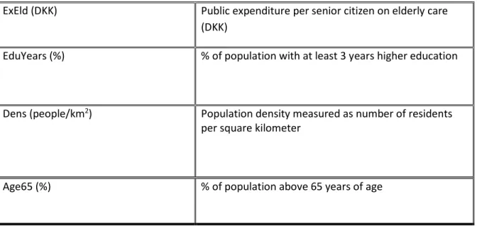
11 ExEld (DKK) Public expenditure per senior citizen on elderly care

(DKK)

EduYears (%) % of population with at least 3 years higher education

Dens (people/km2_{) Population density measured as number of residents}

per square kilometer

Age65 (%) % of population above 65 years of age

The log of annual income per municipality, log(𝑦), was chosen for this paper since the purpose to see how inequality and which factors of inequality could potentially affect economic growth. The average income growth rate of a municipality is a good indicator to show economic

wellbeing of said municipality. The income that was taken was the pre-tax income for the working population aged 14+ in Denmark.

Figure 3 demonstrates that there exists a positive correlation between average income growth and Gini coefficient for the Danish municipalities between 2008-2016. Most municipalities group around the 1.56 percent income growth rate, and a Gini coefficient of 25.7. One of the major outliers in this figure is the municipality of Gentofte, who in 2015 reported an income growth of 15.33 percent and a Gini coefficient of 43.97. Gentofte is again an outlier posting a -5.23 percent decrease in 2016 and Gini coefficient of 47.77. The last outlier is the municipality of Hørsholm who reported a -8.10 percent decrease in income in 2008 with a Gini coefficient of 37.51, but picked up two years later with 15 percent increase in income in 2010. Similar figures showing positive relationships between the 90/80 income ratio and the 50/10 income ratio versus annual income growth can be found in the appendix under Figure 7 and Figure 8.

12

Figure 3: Gini Coefficient vs Annual Income Growth in Danish

Municipalities 2008-2016

For measure of inequality, the Gini coefficient Gini, which is a measure of statistical dispersion made to measure the income distribution on a national or regional scale, is used. The Gini coefficient lies on a scale between 0 and 1, where 0 signifies perfect equality while 1 signifies perfect inequality although for the purpose of this paper StatBank Denmark has multipled the coefficient by 100, leading to 0 signifying perfect equality while 100 signifies perfect inequality. Furthermore, as has been done in Rooth and Stenberg (2008) and Cialani (2014) the income share ratios of the 50th _{and 10}th _{income deciles help us see the effect of income inequality at}

the lower end of the income distribution. Similarly, the 90th _{and 80}th _{income ratio will be used}

13

Earlier studies on similar fields suggest that local policy making has an effect on growth rate of average income (Gleaser et al., 1995; Helms, 1995; Aronsson et al., 2001). The effects of local spending are encapsulated with the variables of Exedu, Exchild, Exeld, and Tax. The variables

Exedu, Exchild, and Exeld, to a certain extent, cover local public expenditure of overall Danish

national policy in terms of local municipality spending. The variable Tax is given by the municipality income tax rate. Helms (1985) finds that taxes have a negative effect on the income growth rate on 48 of 50 states in the USA. William Gale (2014) also did a study on the impact of income taxes on economic growth in the USA and like Helms, found that taxes have either negative or negligible effect on economic growth.

Public expenditure is controlled for with the variables of ExEdu, the amount of public expenditure spent per pupil, ExEld, the amount of public expenditure spent per elderly, and

ExChild, the amount of public expenditure spent per child; all done per municipality. Aronsson

et al. (2001) found that public expenditure per capita does not have a significant impact on income growth on a county level, as did Barro (1991) on a national level.

Human capital in the form of education would also be expected to increase the average income of an area. The variables which control these parameters are EduYears, the share of population with at least a bachelor’s degree. Papers by Jamison et al. (2007) and Krueger and Lindahl (2000) both corroborate that more years in higher education positives correlates to higher levels of income growth.

The variables of Dens and Age65 are used, in line with papers such as Nahum (2005) and Cialani (2014), in order to control for the degree of urbanization and the age structure of the

14

C.

Descriptive statistics

Table 2 provides descriptive statistics of all the dependent and independent variables. Table 2.1 is a condensed version of Table 2 showing more vital descriptive statistics. As can be seen from the table the mean value of the Gini coefficient across all municipalities from the 2008-2016 is 25.70. The values across municipalities and over time, range from 20.40 to 47.77. The Gini coefficient of 47.77 belongs to Denmark’s wealthiest municipality Gentofte in the year 2016. Gentofte throughout the years of 2008-2016 consistently reported the highest Gini coefficient out of all other municipalities, while also reported the highest average income for the years of 2008-2016 implying a correlation between the two. To compare extremes, the lowest Gini coefficient of 20.40 belongs to the municipality of Egedal. Egedal was consistently near the bottom reported Gini coefficient throughout 2008-2016, and was placed into the top 15 average highest incomes for the years 2008-2016. This shows a contrasting relationship with that of Gentofte since Egedal’s Gini coefficient is less than 27 than that of Gentofte’s despite that both of them rank in the top 15 municipalities with highest income in Denmark. The lowest earning municipality was Langeland which was on average the bottom earning Danish

municipality across 2008-2016. Langeland also placed consistently near the bottom of the Gini coefficient distribution with all their Gini coefficients landing in the bottom 100 out of all 882 observations of all Gini coefficients. A reason for this could be that Langeland is an isolated small island, and so is not connected to the large main islands of Denmark.

Table 2.1: Condensed Descriptive Statistics of Danish Municipalities

2008-2016

Variable Mean Std. Dev. Min Max Observations

Income (DKK) Overall 290550.3 48412.32 2117424 611952 882

15 BotIncome Overall 2.870707 7.269899 -140.8272 62.97438 882

Tax (%) Overall 25.21497 0.9085934 22.5 27.8 882

EduYears (%) Overall 13.99683 5.051552 7.822643 34.9789 882

Gini Overall 25.70474 3.53131 20.4 47.77 882

There also exists seems to exist a relationship between geographic location and income as can be seen in Table 3 (appendix). Thirteen of the top fifteen highest earning municipalities are all located in the Danish Capital Region, while the Southern Danish region holds three of the five lowest earning municipalities in Denmark. It is also worth noting that the municipalities with the top ten highest Gini coefficients are all located in the Danish Capital Region, indicating a geographical bias when it comes to income equality.

Turning to the other indicators of income inequality in Table 2.1 we can see that for the top income ratios, that of 90/80, the mean is 1.53 with a max value of 3.04 and a min value of 1.29. Following the trend of Gini coefficient and average income, the highest 90/80 ratio belongs to the municipality of Gentofte, which was also the highest earning municipality throughout the study. The lowest 90/80 ratio of 1.29 belongs to the municipality of Tårnby. Briefly looking at the bottom inequality ratio of 50/10, it shows the mean to be around 2.78, with a max of 62.97 and a min of -140. The reason for a negative number is because the StatBank Denmark

recorded some of the bottom decile incomes as negative. Ignoring these anomalous negative numbers, we see the highest bottom inequality ratio of 62.97 belongs to the municipality of Hjørring, while the minimum lower income ratio of 1.91 belongs to Læsø, which ranks at 3rd

16

Looking at tax rates, we see that the mean tax rate is 25.21 percent throughout the years of 2008-2016. The range of tax rates is from 22.50 to 27.80, with the lowest belonging to Rudersdal for the years 2014, 2015 and 2016, which is also one of the highest earning

municipalities throughout the studies. The highest tax rate of 27.80 belongs to Langeland, the lowest earning municipality throughout the years 2008-2016.

For the share of the population with at least a bachelor’s degree, the mean share of the population was 14 percent, with a minimum percent of 7.82 percent and the highest share of 35 percent. The lowest share belongs to Lolland in 2008, a sparsely populated island in Denmark’s southern region who rank among the bottom of the income distribution. The highest of 35 percent Frederiksberg in 2016, a municipality located in the heart of Copenhagen with a high density of educational institutions.

17

IV. Methodology

A.

Econometric Model

For this paper panel data analysis was the chosen method asses the data. Panel data allows for the use of cross-sectional and time-series dimensions, meaning that data can provide

information across individuals and over time.

The regression equation, with Gini coefficient as the measure of income inequality is

Equation 1: Regression Model Using Gini as Show of Inequality

𝑙𝑜𝑔(𝑦

) = 𝛼 + 𝛿

𝐺

+ 𝛿

𝑇𝑎𝑥

+ 𝛿

𝐸𝑥𝐸𝑑𝑢

+ 𝛿

𝐸𝑥𝐶ℎ𝑖𝑙𝑑

+ 𝛿

𝐸𝑥𝐸𝑙𝑑

+ 𝛿

𝐸𝑑𝑢𝑌𝑒𝑎𝑟𝑠

+ 𝛿

𝐴𝑔𝑒65

+ 𝛿

𝐷𝑒𝑛𝑠

+ 𝜀

In this study Gini coefficient, as well as top and bottom inequality ratios, those of 90/80 and 50/10, be used as indicators of income inequality, as was done in Nahum (2005) and Cialani (2013). As these variables are measures of income inequality, they are set to be switched with the Gini coefficient as shown in Equation 2 and Equation 3.

Equation 2: Regression Model Using TopIncome as Show of Inequality

𝑙𝑜𝑔(𝑦

) = 𝛼 + 𝛿

𝑇𝑜𝑝𝐼𝑛𝑐𝑜𝑚𝑒

+ 𝛿

𝑇𝑎𝑥

+ 𝛿

𝐸𝑥𝐸𝑑𝑢

+ 𝛿

𝐸𝑥𝐶ℎ𝑖𝑙𝑑

+ 𝛿

𝐸𝑥𝐸𝑙𝑑

+ 𝛿

𝐸𝑑𝑢𝑌𝑒𝑎𝑟𝑠

+ 𝛿

𝐴𝑔𝑒65

+ 𝛿

𝐷𝑒𝑛𝑠

+ 𝜀

Equation 3: Regression Model Using BotIncome as Show of Inequality

𝑙𝑜𝑔(𝑦

) = 𝛼 + 𝛿

𝐵𝑜𝑡𝐼𝑛𝑐𝑜𝑚𝑒

+ 𝛿

𝑇𝑎𝑥

+ 𝛿

𝐸𝑥𝐸𝑑𝑢

+ 𝛿

𝐸𝑥𝐶ℎ𝑖𝑙𝑑

+ 𝛿

𝐸𝑥𝐸𝑙𝑑

+ 𝛿

𝐸𝑑𝑢𝑌𝑒𝑎𝑟𝑠

+ 𝛿

𝐴𝑔𝑒65

+ 𝛿

𝐷𝑒𝑛𝑠

+ 𝜀

18

A final model that will be used will incorporate both TopIncome and BotIncome to see how income affects simultaneously at the top and bottom end of the income distribution.

Equation 4: Regression Model Using BotIncome and TopIncome as

Show of Inequality

𝑙𝑜𝑔(𝑦

) = 𝛼 + 𝛿

𝐵𝑜𝑡𝐼𝑛𝑐𝑜𝑚𝑒

+ 𝛽

𝑇𝑜𝑝𝐼𝑛𝑐𝑜𝑚𝑒

+ 𝛿

𝑇𝑎𝑥

+ 𝛿

𝐸𝑥𝐸𝑑𝑢

+ 𝛿

𝐸𝑥𝐶ℎ𝑖𝑙𝑑

+ 𝛿

𝐸𝑥𝐸𝑙𝑑

+ 𝛿

𝐸𝑑𝑢𝑌𝑒𝑎𝑟𝑠

+ 𝛿

𝐴𝑔𝑒65

+ 𝛿

𝐷𝑒𝑛𝑠

+ 𝜀

The dependent variable of 𝑦 (annual income DKK) will be logged in order to more easily

interpret its coefficient when the panel regressions are run. As the all the independent variables are not transformed, the relationship between the dependent and independent is logarithmic-linear. This allows for the dependent variable to be interpreted as a percent increase (or decrease) rather than units of Danish Kronor. Therefore, the interpretation of the coefficients of my four models would be

%∆𝑦 = 100 ∗ (𝑒𝛿𝑥_{− 1) or %∆𝑦 = 100 ∗ 𝛿}

𝑥∗ ∆𝑥 for simplicity.

B.

Endogeneity Issue

The effects of income inequality on income growth could raise problems of endogeneity. Endogeneity is an issue where an explanatory variable could be correlated with the error term. Potential endogeneity issues arise from the inequality indicators; the estimated effect of income inequality on income growth could be biased via correlation between the income inequality indicators and the error term. If independent variables are endogenous and correlated with the error term, then it is possible that our OLS (ordinary least squares)/ FE (fixed effects) results could are biased and inconsistent.

19

There are multiple ways in dealing with endogeneity such as 2/3 SLS (step least square)

regressions or System-GMM. This being said, no procedures to rectify the issue of endogeneity in my sample; simply stating that such bias could be present in my results, although not likely.

C.

Tests for Model

Firstly, as this will be a panel data model due to having both cross-sectional and time-series components, the next question that arises is to which type of panel data model best fits the econometric analysis. When dealing with panel data multiple analysis models exist for regression analysis; the two most prominent being fixed effects models and random effects model. Several tests will be performed on previously stated models to see which is optimal for this study.

The Hausman test is a statistical hypothesis test, which tests to see if there exists a correlation between the errors and regressors in the model. Thus, the two hypotheses are:

𝐻0: 𝑅𝑎𝑛𝑑𝑜𝑚 𝐸𝑓𝑓𝑒𝑐𝑡𝑠 𝑀𝑜𝑑𝑒𝑙 𝑖𝑠 𝑆𝑢𝑖𝑡𝑎𝑏𝑙𝑒

𝐻1: 𝐹𝑖𝑥𝑒𝑑 𝐸𝑓𝑓𝑒𝑐𝑡𝑠 𝑀𝑜𝑑𝑒𝑙 𝑖𝑠 𝑆𝑢𝑖𝑡𝑎𝑏𝑙𝑒

Running the hausman test on Stata using Equation 1, leads us to the result shown in Figure 4 (appendix); using 𝛼 = 0.01 we can reject the null hypothesis at the 1% significance level and conclude that the fixed effects model is suitable for this data since 𝑝 < 0.01.

The fixed effects model is an econometric model which allows for the control of omitted variables/ unobserved heterogeneity that could otherwise influence results. Dummy variables for space and time (Danish municipalities and years in my case) are fixed to deal with omitted

20

variable bias that could occur in standard regressions. The left over ‘within’ variations could help identify casual relationships.

Next, multicollinearity was tested for in the model. A correlation table, Table 4 (appendix), was made to see if any of the explanatory variables related to one another. As can be seen, since no variable exceeds the value of ±0.8 (excluding constant term) we can conclude there is no multicollinearity in Equation 1.

A further test for multicollinearity was done in the form of VIF (Variance Inflation Factor). As can be seen from Table 5 (appendix), none of the variables exceed VIF of ten, therefore we can conclude again that no multicollinearity is present.

To test for autocorrelation a Wooldridge test was used. The two hypotheses for this test are: 𝐻₀: 𝐴𝑢𝑡𝑜𝑐𝑜𝑟𝑟𝑒𝑙𝑎𝑡𝑖𝑜𝑛 𝑖𝑠 𝑛𝑜𝑡 𝑝𝑟𝑒𝑠𝑒𝑛𝑡

𝐻₁: 𝐴𝑢𝑡𝑜𝑐𝑜𝑟𝑟𝑒𝑙𝑎𝑡𝑖𝑜𝑛 𝑖𝑠 𝑝𝑟𝑒𝑠𝑒𝑛𝑡

As seen in Figure 5 (appendix), using 𝛼 = 0.01 we can reject the null hypothesis at the 1% significance level and conclude that autocorrelation is present in this model since 𝑝 < 0.01.

To test for heteroscedasticity a Breusch-Pagan test was used. The two hypotheses for this test are:

𝐻0: 𝐻𝑒𝑡𝑒𝑟𝑜𝑠𝑐𝑒𝑑𝑎𝑠𝑡𝑖𝑐𝑖𝑡𝑦 𝑖𝑠 𝑛𝑜𝑡 𝑝𝑟𝑒𝑠𝑒𝑛𝑡

𝐻1: 𝐻𝑒𝑡𝑒𝑟𝑜𝑠𝑐𝑒𝑑𝑎𝑠𝑡𝑖𝑐𝑖𝑡𝑦 𝑖𝑠 𝑝𝑟𝑒𝑠𝑒𝑛𝑡

As seen in Figure 6 (appendix), using 𝛼 = 0.01 we can reject the null hypothesis at the 1% significance level and conclude that heteroscedasticity is present in this model since 𝑝 < 0.01.

21

Since heteroscedasticity and autocorrelation were both detected in the model for Equation2 _1,

an appropriate solution to counteract these deficiencies is using robust estimators. Luckily, there exists a function on Stata that can automatically run robust fixed effects regression.

22 _{The same tests were ran for when the income ratios of 90/80 and 50/10 were used as a measure of inequality}

22

V. Conclusions

A.

Empirical Findings

Firstly, a robust fixed effects regression is run on Equation 1 where Gini coefficient is the indicator of income inequality; shown in Table 6

Table 6: Coefficient Table of Panel Regressions

with Log(Income) as Dependent Variable

Variable Model 1 (Gini) Model 2 (90/80 Income Ratio) Model 3 (50/10 Income Ratio) Model 4 (50/10 and 90/80 Income Ratio) Gini 0.0013575 - - - TopIncome (90/80) - 0.2199983*** - 0.2185644*** BotIncome (50/10) - - 0.0003424** 0.000255** Tax (%) 0.002556 0.0039316 0.0015467 0.0042149 Age65 (%) 0.0153455*** 0.0139974*** 0.0151835*** 0.0140897*** EduYears (%) 0.0337278*** 0.0276174*** 0.034326*** 0.027665*** ExChild (DKK) -6.40e-07 -1.83e-07 -7.85e-07* -1.65e-07

ExEld (DKK) 2.45e-07 6.54e-07** 1.84e-07 6.86e-07**

ExEdu (DKK) 1.34e-07 4.17e-07** 1.49e-07 4.19e-07**

Dens (people/km2_{) -2.48e-06 -7.19e-06** -1.75e-06 -7.02e-06**}

Constant 11.70814*** 11.43111*** 11.76925*** 11.42043*** R2 F value Prob > F Observations 0.5714 211.70 0.0000*** 882 0.5995 314.13 0.0000*** 882 0.5712 226.32 0.0000*** 882 0.5974 281.82 0.0000*** 882

Note: * signifies significance at the 0.1 level, ** at the 0.05 level, and *** at the 0.01 level

From what is seen in Table 6, overall Model 1 has an R2 _{of 0.57 indicating a moderate}

23

growth, thus a one-unit increase in Gini coefficient would lead to a 0.136 percent increase in income. This would be in line with the findings of and Rooth and Stenberg (2010) who also found in his models that Gini was insignificant and positive, but unlike the results of Cialani (2014) who found Gini to be significant and positive in her models.

One of the more striking results of these regressions is that Gini is insignificant. This could be for several reasons, first and foremost the way in which the Gini was calculated by the StatBank Denmark. Since StatBank Denmark do not provide data in order to calculate Gini what was used instead was their listed data for Gini coefficient, which is just a value from 0-100 for each municipality for each year. It is not revealed how this number is obtained, what their metric for income was (pre-tax vs post-tax, 14+ or 14-64, subsidies, welfare and pensions included?) and could be skewed in this way. Another reason could be that I have made an error in calculations and processing of the data, although this is unlikely since the rest of my results are sound. Finally, it could be that my results are indeed correct and that Gini in this case is not statistically significant for Danish municipalities in the selected time span and a correlation does not exist, although the other measures of income inequality contrast this notion.

The variable Tax, is seen to be positively correlated with income growth, although again it is not significant in this regression. This differs from the findings of Helms (1985) who found a

negative relationship between taxation and economic growth in 48 of 50 states in the United States. My results, however, are more in line with those of Gale (2014) who found that either negligible or negative insignificant relationships exist for taxes and growth in the United States.

Next, the variable Age65 shares a positive relationship and significant relationship with income. For a one percent increase in the share of the population over the age of 65 we can predict that annual income would grow at about 1.5 percent. This differs from the findings of Cialani who found a negative relationship between Age65 and income growth although it was insignificant

24

in her case. However, this corroborates with the findings of Nahum (2005) who finds a positive and significant correlation between income and share of the population above 65 for Swedish counties.

The variable to encompass human capital, EduYears, unsurprising was positively correlated with income growth and is statistically significant. A one percent increase in the share of the

population with at least a bachelor’s degree would increase annual income by about 3.3 percent. This is in line with most literature (Cialani 2012; Jaimson et al. 2007; Kruegar and Lindahl 2000) that finds a strong positive correlation between education and income growth.

Local public expenditure in the forms ExChild, ExEdu, and ExEld all turn out to be insignificant in this particular model, with only ExChild exhibiting a negative correlation with income. These results are in line with the findings of Barro (2000) and Aronsson et al. (2001), both of whom found that public expenditure had an insignificant impact on income growth, on a county and national level.

The last variable Dens, shares a negative but insignificant relationship with income growth. This result is similar to Cialani (2014) who found density and income growth to be negatively

related, although in her case, the variable was statistically significant.

Subsequently, a robust fixed effects regression is run again but with Model 2 (90/80 income ratio). The robust regression for Top Income (90/80 income ratio) varies quite a bit from that of when the Gini coefficient was used as the measure of inequality. The R2 _{has slightly increased to}

0.60 from 0.57 in the previous regression, again indicating a moderately strong correlation. The first major difference is that TopIncome is highly significant and positively correlated with income growth. In this case, a one-unit increase in the 90/80 income ratio would increase

25

annual income by 21.9 percent. This result is very interesting but not surprising seeing as many papers (Roothe and Stenberg 2010; Cialani 2014) also corroborate how income growth for top earners is much more than that of the average and bottom earners.

Tax again is statistically insignificant for this regression although the coefficient now

experiences a negative relationship with income growth. As with the previous regression both

EduYears and Age65 have a positive and significant relationship with income growth.

Interestingly, both coefficients in this case are lower than that of when Gini was used as a measure of income inequality.

Looking at the variables for public expenditure, we see that ExChild is negative but

insignificantly correlated to income, while ExEld and ExEdu are both positively correlated to income and significant at the 0.1 and 0.05 level of significance. Although this contradicts that findings of Barro (2000) and Aronsson et al. (2001), it does fall in line with the findings of Cialani (2014) who found all three of the public expenditure variables to be positive and significant for the TopIncome in Swedish municipalities.

Dens is negatively correlated with income growth and significant at the 0.1 and 0.05 level. This

suggests that a one-unit increase in population density, leads to a 0.000719 percent decrease in income growth. This is a similar finding to Cialani (2014) who found a negative and significant relationship between income and density, across all models.

Next, a robust fixed effects regression is run again for Model 3 (50/10 income ratio) with

TopIncome as the indicator of income inequality. The robust regression for Model 3 (the 50/10

income ratio) has an R2 _{of 0.57, same as the regression for Gini and lower than that of}

TopIncome, although all are very similar and imply a moderate relationship exists. As with TopIncome, the coefficient for BotIncome is positive and statistically significant at the 0.1 and

26

0.05 level. In this case, a one-unit increase in BotIncome leads to a 0.034 percent increase in income growth. This is much less than that of TopIncome and shows a bias towards income growth for those at the top of the income distribution.

Once again Tax is shown to be positive but insignificantly correlated with income. Both Age65 and EduYears are positively correlated and significant with income and both the coefficients are higher than that of TopIncome.

For the variables of public expenditure, ExChild is negative correlated and statistically significantly at the 0.1 and 0.05 level, while the other ExEld and ExEdu are both positively correlated to income but statistically insignificant. Interestingly, this is the opposite of the regression results of TopIncome where ExChild was statistically insignificant, but ExEld and

ExEdu were both statistically significant. Dens is once again negatively correlated with income

growth, but in this case it is not statistically significant.

Finally a robust regression is run for Model 4, which combines TopIncome and BotIncome as measures of inequality, this way both ends of the income distribution curve are shown simultaneously. Both TopIncome and BotIncome are significant for the regression, although

BotIncome is not significant at the 0.01 level. The coefficients again show a bias towards TopIncome, whose coefficient is much larger than that of BotIncome’s.

Both EduYears and Age65 are again significant with positive coefficients. Interestingly for public expenditure, it can be seen that both ExEld and ExEdu are significant. Again, ExChild is negative and not significant for this model. The coefficients are also the highest for Model 4, than in all other models. Dens is shown be significant for the 2nd _{time again with a negative coefficient.}

27

From analyses of all three of the robust regressions presented we can draw conclusions on income growth in Danish municipalities. From TopIncome and BotIncome regression results we can see how income growth is biased towards the rich, where the coefficient for Topincome indicated a 21.9 percent increase in income with a one-unit increase in the 90/80 income ratio, compared to the 0.034 percent increase in income with a one-unit increase in the 50/10 income ratio. This is also the case when combining both TopIncome and BotIncome in Model 4.

Another interesting note is that in Model 3 and Model 4, the BotIncome ratio is positive but miniscule, suggesting a positive but small relationship between income growth and income equality. This is however not the case for Cialani (2014) and Voichovksy (2005) who found that bottom end income earners shared a small but negative relationship with income inequality. In the case of Rooth and Stenberg (2005), for Swedish labour market, it was found that the

bottom end inequality and income equality shared a positive relationship although it was insignificant for them. A theory for these results could be that for the case of Cialani (2014) and Voichovsky (2005), the segregation of those with low income, who are isolated in their ‘ghetto’ neighborhoods where the level of education is low, access to health facilities is scarce, and infrastructure could be underdeveloped. This is not so much the case for Denmark where those with low income are not as segregated and are more acclimated with Danish society as a whole and enjoy the benefits of rich education, and strong economic policies for lower end earners.

Another reason for the discrepancy of income growth for TopIncome and BotIncome could be migration of educated individuals to another municipality. For example, it could be possible that a highly educated individual from a certain region decides to move to a municipality with greater opportunity or work such as Copenhagen, and the destination municipality then see the increase of their income growth while the municipality the individual departed from does not reap these benefits or show up in the data.

28

As expected, EduYears was positively correlated and significant in all four models, with the highest coefficient found in the BotIncome model. The coeffcieint suggests a one percent increase in population share with at least bachelor’s degree increases income by 3.4 percent, while for TopIncome it increases only by 2.7 percent. This shows how the vital role education can have in alleviating poverty and increasing income in lower income areas in Denmark. This can also show how at the higher end of the income distribution education is as vital to further increase income.

Age65 (the share of the population above the age of 65) was the only other variable to be

positively correlated and significant in all four models. This could be explained by Denmark’s generous pension system which could pay up to elderlies up to 850,000 DKK annually and could greatly skew results as on the StatBank website it is not clear if pensions are included in

disposable income, although this should not affect income growth it remains static.

The variable Tax showed to have no statistical impact on income growth which has been found in other studies (Helms 1985; Gale 2014), although their study was conducted in the United States. This is different from the findings of Cialani (2014) who found a significant and negative relationship between income growth and taxes in Swedish municipalities. It could be possible that Denmark, unlike Sweden, has been laxer in their taxation of high earning individuals, leading to this trend.

Public expenditure, captured by ExEdu, ExEld and ExChild were also expected to be insignificant, but only the model with Gini showed this to be the case. Surprisingly, ExEld and ExEdu were both statistically significant for the TopIncome regressions and for Model 4. For ExChild was only significant for BotIncome and was negatively correlated.

29

As for population density, it was significant for TopIncome and for Model 4 were it was negatively correlated. This is in line with Cialani (2014) and shows that working and living in highly densely populated, such as Copenhagen or Fredriksberg, doesn’t necessarily correlate to an increase in income, but instead leads to a decrease in income.

Another conclusion that can be drawn from these results is that Gini on its own is not sufficient to capture the effects of income inequality on income growth and the full complexity of the relationship.

On a holistic note, it can be seen that a tradeoff does not exist for income growth and income inequality. In this sense, a high-income equality could be beneficial for income growth while a low-income inequality could be detrimental for income growth, at least in the case for Danish municipalities. High income inequality in municipalities with individuals at the high end of the income distribution see a much higher increase in income growth than municipalities with high income inequality and individuals at the lower end of the income distribution.

Since Denmark is a very developed nation, these results coincide with the papers of Barro (2000) and Voitchovsky (2005) who find that in more developed nations, income inequality leads to income while in poorer nations income inequality leads to a decrease in income growth. Their samples included countries with a wide range of Gini coefficients such as 63.4 (South Africa) and Mexico (48.2). In comparison, Denmark’s average Gini coefficient through the study was 25.7 with a standard deviation of 3.53. It could be possible that if a similar study was done on municipalities is another less developed nation such as Mexico or South Africa it could be found that even the top earning municipalities could be negatively affected by income inequality.

30

These results also show that redistributive policies, such as welfare and progressive taxation, will likely hinder growth in Danish municipalities, with higher impediment of economic growth for those at top end of the income distribution, and lower impediment for those at the lower end of the income distribution.

B.

Limitations and Possibilities for Further Research

As stated in the Data and Framework section of the paper, one of the limitations of this study is that not all of Denmark’s population was accounted for. Although only about 2% of Denmark’s population is missing in this study, the missing regions of Faroe Island, Greenland, and

Ertholomene are historically poorer regions of the Kingdom of Denmark and therefore, even if just slightly, could have skewed the results of the study.

Another limitation was the lack of data available. Although StatBank Denmark has a

comprehensive amount of data already, most data for municipalities started to be recorded in 2007, because that was when the new municipality reform occurred in Denmark. This greatly restricted the years in which this study could be conducted in.

In the previous studies, such as those of Cialani (2014), Rooth and Stenberg (2012), and Nahum (2005) all use top one, five, ten, 15, and 20 percent earner as a measure of income inequality, as it a good measure of the high end of the income distribution. Unfortunately, such data was unavailable to me, as when I emailed StatBank Denmark about the availability of such data, their response was the data is available to students with an association to a Danish university or made through a payment.

31

The chosen spatial unit of municipality could also be a limitation of the study. As mentioned previously, an individual who commutes to a different municipality would not care about the income growth in the municipality where he lives rather where he works. The Swedish statistics bureau has managed to account for these labor commuting routes and arranged all Swedish municipalities into labor markets which are more economically encompassing than

administratively divided municipalities. Unfortunately, StatBank Denmark does not do the same with Danish municipalities. An interesting variable that could account for the shortcomings of the municipality spatial unit in a future study, could be a variable that encompasses the effects of the neighborhood effect. A dummy variable, for example, that equals 1 when a neighboring municipality has an annual two percent growth rate or above, and a 0 when a neighboring municipality has less than an annual two percent income growth rate.

32

VI. References

Aghion, Philippe, Eve Caroli, and Cecilia García-Peñalosa . “Inequality and Economic Growth: The

Perspective of the New Growth Theories.” Journal of Economic Literature 37, no. 4, December 1999, pp.

1615–1660

Alan B. Krueger & Mikael Lindahl. "Education for Growth: Why and for Whom?," Journal of Economic

Literature, American Economic Association, vol. 39, no.2 Dec. 2001 , pp. 1101-1136.

Alesina, Alberto, and Dani Rodrik. “Distributive Politics and Economic Growth.”Quarterly Journal of

Economics, vol. 109, no. 2, May 1994, pp. 465–490.

Aronsson, Thomas, et al. “Union Wage Setting and Capital Income Taxation in Dynamic General Equilibrium.” German Economic Review, vol. 2, no.2, May 2001, pp. 141-175.

Atkinson, A. B.; Søgaard, J.E. The long-run history of income inequality in Denmark: Top incomes from 1870 to 2010, EPRU Working Paper Series, No. 2013-01.

Barro, Robert J. “Inequality and Growth in a Panel of Countries.” Journal of Economic Growth, vol. 5, no. 1, 2000, pp. 5–32.

Birdsong, Nicholas. “The Consequences of Economic Inequality.”Sevenpillarsinstitute.org (website), 5 Feb. 2015, sevenpillarsinstitute.org/case-studies/consequences-economic-inequality#_ftnref33.

Causa, Orsetta, Mikkel Hermansen, Nicolas Ruiz, Caroline Klein, Zuzana Smidova. “Inequality In Denmark Through The Looking Glass.” Economics Department Working Papers, no. 1341, 2016.

Cialani, Catia. “Growth and Inequality: A Study of Swedish Municipalities. Thesis. Dalarna University, 2013.

Fi, Hongyi, and Heng-fu Zou. “Income Inequality Is Not Harmful for Growth: Theory and Evidence.” Review of Development Economics, vol. 2, no. 3, Oct. 1998, pp. 318–334.

33 Glaeser, Edward L, Jose A Scheinkman, and Andrei Shleifer. “Economic Growth in a Cross-Section of

Cities.” Journal of Monetary Economics 36, no. 1, 1995, pp. 117-143.

Graham, Paul. “Economic Inequality: The Short Version.” Economic Inequality: The Short Version, Jan. 2016, pualgraham.com/sim.html.

Jamison, Eliot A., et al. “The Effects of Education Quality on Income Growth and Mortality Decline.” Economics of Education Review, vol. 26, no. 6, Dec. 2007, pp. 771–788.

Local, The. “Denmark's One Percent Problem.” The Local, The Local, 1 Sept. 2014,

www.thelocal.dk/20140901/denmarks-one-percent-problem.

Papanek, Gustav F, and Oldrich Kyn. “The Effect On Income Distribution of Development, the Growth Rate and Economic Strategy.” Journal of Development Economics, vol. 23, no. 1, 1986, pp. 55–65.

Paukert F. ”Income distribution at different levels of development: a survey of evidence”. tnt. Lab. Rev. 108, 1973, pp. 97-125.

Ram, Rati. “‘NOMINAL’ AND ‘REAL’ INTERSTATE INCOME INEQUALITY IN THE UNITED STATES: SOME ADDITIONAL EVIDENCE.” The Review of Income and Wealth, vol. 41, no. 4, Dec. 1995, pp. 399–404.

Rooth, Dan-Olof, and Anders Stenberg. “The Shape of the Income Distribution and Economic Growth- Evidence from Swedish Labor Market Regions.” Scottish Journal of Political Journal, no. 59, ser. 2, May 2012, pp. 196-223. 2.

Tsakloglou, Panos. “ASPECTS OF POVERTY IN GREECE.” Review of Income and Wealth, vol. 36, no. 4, Dec. 1990.

Voitchovsky, Sarah. “Does the Profile of Income Inequality Matter for Economic Growth?” Journal of

Economic Growth, vol. 10, 2005, pp. 273–296.

Wilkinson, Richard G, and Kate Pickett. “The Spirit Level: Why Greater Equality Makes Societies Stronger”. New York: Bloomsbury Press, 2010. Print.

34

VII. Appendix

A.

Tables

Table 2:

Descriptive Statistics of Danish Municipalities 2008-2016

Variable Mean Std. Dev. Min Max Observations

Log (Income) (variable used in models) Overall 12.56819 0.1440811 12.2896 13.32441 882 Income (DKK) Overall 290550.3 48412.32 2117424 611952 882 IncomeGrowth (%) (variable not used in models) Overall 1.561378 2.062082 -8.100158 15.33142 882 Gini Overall 25.70474 3.53131 20.4 47.77 882 TopIncome Overall 1.529793 0.1703462 1.29409 3.040685 882 BotIncome Overall 2.870707 7.269899 -140.8272 62.97438 882 Tax (%) Overall 25.21497 0.9085934 22.5 27.8 882 EduYears (%) Overall 13.99683 5.051552 7.822643 34.9789 882 Age65 (%) Overall 19.03176 3.703162 10.14269 35.98001 882 ExChild (DKK) Overall 35691.00 6884.336 23518 63955 882 ExEld (DKK) Overall 52318.13 7542.184 34271 88491 882

35

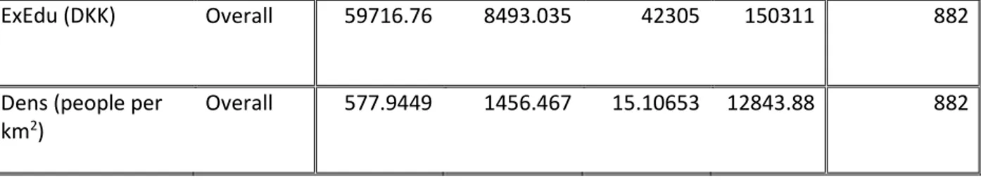
ExEdu (DKK) Overall 59716.76 8493.035 42305 150311 882

Dens (people per km2₎

Overall 577.9449 1456.467 15.10653 12843.88 882

Table 3: Danish Municipality Regions Sorted by Average Income

2008-2016

36 Rebild 287700 No No Odder 287302 No No Ringsted 287211 No No Høje-Taastrup 286592 Yes No Hvidovre 286376 Yes No Rødovre 286320 Yes No Hedensted 286018 No No Stevns 285422 No No Holbæk 284762 No No Sorø 284521 No No Copenhagen 284277 Yes No Billund 283029 No Yes Fredericia 281934 No Yes Aarhus 280976 No No Syddjurs 280477 No No Esbjerg 279569 No Yes Viborg 279342 No No Halsnæs 279151 No No Faxe 278518 No No Herning 277749 No No Horsens 277694 No No Holstebro 275927 No No Næstved 275451 No No Kerteminde 274092 No Yes Ringkøbing-Skjern 273581 No No Kalundborg 273559 No No Ikast-Brande 272343 No No Varde 272046 No Yes Lemvig 271464 No No Aalborg 270797 No Yes Vejen 268671 No No Sønderborg 268443 No Yes Svendborg 268145 No Yes Randers 267807 No No Haderslev 267533 No No Nyborg 267110 No No Mariagerfjord 266499 No No Struer 266269 No No Assens 266202 No Yes Slagelse 265716 No No Aabenraa 265683 No Yes Albertslund 265366 Yes No Frederikshavn 265150 No No Brøndby 265001 Yes No Jammerbugt 264449 No No Brønderslev 264241 No No Nordfyns 263813 No Yes Hjørring 263215 No No

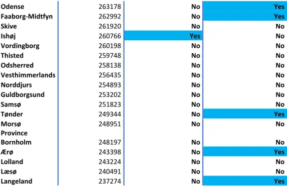
37 Odense 263178 No Yes Faaborg-Midtfyn 262992 No Yes Skive 261920 No No Ishøj 260766 Yes No Vordingborg 260198 No No Thisted 259748 No No Odsherred 258138 No No Vesthimmerlands 256435 No No Norddjurs 254893 No No Guldborgsund 253202 No No Samsø 251823 No No Tønder 249344 No Yes Morsø 248951 No No Province Bornholm 248197 No No Ærø 243398 No Yes Lolland 243224 No No Læsø 240491 No No Langeland 237274 No Yes

Table 4: Correlation Table Using Equation 1

Variable Gini Tax Age65 EduYears ExChild ExEld ExEdu Cons

Gini 1.0000 - - - - Tax 0.1737 1.0000 Age65 0.2053 -0.2025 1.0000 EduYears -0.2151 -0.0683 -0.4666 1.0000 ExChild 0.2517 -0.1922 -0.0198 0.0917 1.0000 ExEld 0.2167 0.0072 0.4416 0.0438 -0.0714 1.0000 ExEdu -0.0277 0.0180 -0.3246 -0.2409 0.0400 -0.2060 1.0000 Dens -0.0371 0.0322 0.2073 -0.3809 -0.0591 0.0688 0.0553 1.0000 Constant -0.3734 -0.9482 0.0976 -0.0016 0.0203 -0.2036 -0.0075 -0.0284

38

Table 5: VIF Table Using Equation 1

Variable VIF 1/VIF

EduYears 2.98 0.336094 Gini 2.36 0.424521 Dens 1.89 0.528749 ExChild 1.79 0.558353 Age65 1.65 0.606686 ExEdu 1.46 0.684443 ExEld -1.35 0.739521 Mean VIF 1.92

B.

Figures

Figure 4: Hausman Test Using Equation 1

Variable Coefficients

RE (b) FE (B) Difference (b-B) S.E. Sqrt (diag(V_b-V_B)

Gini 0.000884 0.0013575 -0.0004735 0.0002144

Tax -0.004841 0.002556 -0.00304 -

Age65 0.0146702 0.0153455 -0.0006753 0.000077

39

ExChild -7.00e-07 -6.40e-07 -6.02e-08 7.21e-08

ExEld -2.75e-07 2.45e-07 -5.20e-07 6.92e-08

ExEdu 2.67e-07 1.34e-07 1.32e-07 5.35e-08

Dens -0.0000168 -2.48e-06 -0.0000143 -

𝑇𝑒𝑠𝑡: 𝐻0: 𝐷𝑖𝑓𝑓𝑒𝑟𝑒𝑛𝑐𝑒 𝑖𝑛 𝑐𝑜𝑒𝑓𝑓𝑖𝑐𝑖𝑒𝑛𝑡𝑠 𝑖𝑠 𝑛𝑜𝑡 𝑠𝑦𝑠𝑡𝑒𝑚𝑎𝑡𝑖𝑐

𝑐ℎ𝑖2 (6) = (𝑏 − 𝐵) [(𝑉′ 𝑏− 𝑉𝐵)−1](𝑏 − 𝐵)

= 176.58

𝑃𝑟𝑜𝑏 > 𝑐ℎ𝑖2 = 0.0000

Figure 5: Wooldridge Test for Autocorrelation Using Equation 1

𝑊𝑜𝑜𝑙𝑑𝑟𝑖𝑑𝑔𝑒 𝑡𝑒𝑠𝑡 𝑓𝑜𝑟 𝑎𝑢𝑡𝑜𝑐𝑜𝑟𝑟𝑒𝑙𝑎𝑡𝑖𝑜𝑛 𝑖𝑛 𝑝𝑎𝑛𝑑𝑒𝑙 𝑑𝑎𝑡𝑎 𝐻0: 𝑛𝑜 𝑓𝑖𝑟𝑠𝑡 − 𝑜𝑟𝑑𝑒𝑟 𝑎𝑢𝑡𝑜𝑐𝑜𝑟𝑟𝑒𝑙𝑎𝑡𝑜𝑛

𝐹(1, 97) = 16.554 𝑃𝑟𝑜𝑏 > 𝐹 = 0.0001

Figure 6: Breusch-Pagan Test for Heteroscedasticity Using Equation 1

𝐵𝑟𝑒𝑢𝑠𝑐ℎ − 𝑃𝑎𝑔𝑎𝑛 𝑡𝑒𝑠𝑡 𝑓𝑜𝑟 ℎ𝑒𝑡𝑒𝑟𝑜𝑠𝑐𝑒𝑑𝑎𝑠𝑡𝑖𝑐𝑖𝑡𝑦 𝐻0: 𝑐𝑜𝑛𝑠𝑡𝑎𝑛𝑡 𝑣𝑎𝑟𝑖𝑎𝑛𝑐𝑒

𝑐ℎ𝑖2(1) = 130.05 𝑃𝑟𝑜𝑏 > 𝑐ℎ𝑖2= 0.0000

40

Figure 7: Top Income Ratio vs Annual Income Growth in Danish

Municipalities 2008-2016

41

Figure 8: Bot Income Ratio vs Annual Income Growth in Danish

Municipalities 2008-2016