Analysis of deep water single point moorings: technical report

ANALYSIS OF DEEP WATER SINGLE POINT MOORINGS

August 1970

by John H. Nath

Associate Professor of Civil Engineering Colorado State University

for

Office of Naval Research Grant No. N00014-67-A-0299-0009

11111111111111111

Analytical and numerical studies were made of single point moorings of a large disc buoy in deep water. Waves of different

frequencies and winds of different magnitudes were imposed on moorings of different scopes for nylon ropes. The numerical model results compared favorably with analytical solutions for a straight vibrating string and the buoy motion was validated with the results from a

hydraulic model study. Approximate calculations, based on the straight vibrating string solution, were compared to the numerical results of curved mooring lines of various scopes. The analytical prediction of line tension was from fair to poor but the prediction of the position of the nodes of tension and the natural frequencies of the modes was good. A new method of presenting mooring line tension data in dimen-sionless form is presented that reduces moorings of different frequen-cies and line diameters to a common scale. The versatility of the numerical program was illustrated with two runs for moorings in shallow water with large waves in addition to a computation of line tension, position and velocity for the condition of a wind shift of 180 degrees on the buoy_ The usefulness of the numerical program as a design tool was established.

With gratitude the author acknowledges the support of this research by the Ocean Science and Technology Division of the Office of Naval Research.

The computer work was accomplished at the computer center at Colorado State University. Mr. W. W. Burt provided very able

assistance on programming, particularly the plotting subroutines. Mr. Hin Fatt Cheong provided valuable assistance.

ABSTRACT · · · ii

ACKNOWLEDGEMENTS · · .iii

TABLE OF CONTENTS _{· · iv}

INTRODUCTION · · · 1

Background Information · · · • · · • · 1

Scope of This Study . · · . 3

Review of Recent Literature 4

THEORETICAL CONSIDERATIONS · _{• • • • 8}

Governing Equations for Line MOtion · . 8

Governing Equations for Buoy MOtion · 11

Boundary Conditions . · · · · • . · · • · · • 13

PHYSICAL CHARACTERISTICS OF THE SYSTEM · 15

NUMERICAL RESULTS _{• • 19}

Longitudinal and Transverse Motion of the Line _{• · 19} Buoy t.btion · · · · • · . . · · · . 27

Water Sheave ~

.

· · · . · · 29 Effects From the Environment at Sea • · · · . _{• · • 31} SUMMARY AND CONCLUSIONS · · · · . · · • • . · · · · . · · 37

REFERENCES · · • • 39

TABLES · . 41

FIGURES _{· · · • • · · · 53}

Background Information

This report will present the current status of research into the numerical analysis of the motion of the mooring line and buoy of a single point mooring in the deep ocean for an oceanographic buoy. The work originally started in the summer of 1967 for the Convair Division of General Dynamics and was continued in the summer of 1968. During the academic year 1968-1969 the work was continued by the author on a part time basis at Oregon State University under the auspies of the Office of Naval Research. Such a part time arrangement was continued during the past academic year, also for the Office of Naval Research. The objective of this study has been to develop a flexible numerical program that can be used for design work and for engineering research on the mooring of an oceanographic buoy in deep water with a single line. It was desired that the program be able to handle situations with relatively large scopes as well as taut moorings. The effects from waves, or problems on transients, such as the anchor last

deployment procedure, can be studied. An alternative, or supplemental, approach would have been to consider a solution based on small

perturbations about the equilibrium position of the line. However, such a procedure considers only sinusoidal input functions and the program that was developed was much more flexible in being able to compute results for a wide variety of problems which included certain non-linear effects. For design purposes it would be useful to have both types of solutions.

The numerical program can be considered to exist in two parts -one that determines the static or equilibrium position and tension in the line due to the action of wind, current and gravity and the second part that determines the dynamic tension and motion of the line due to waves or other forcing functions. The first part generates. the initial

conditions for the second part. All loads and system responses are considered to be acting in one plane.

The static part of the work has been described in Refs. 10 and 11 and the dynamic portion of the program has been described in Refs. 11 and 12.

The work has been successful to the point of developing and debugging a program which predicts the position, velocity and tension in all parts of the line and the buoy motion. The forcing function can be a wave of any form, providing the water particle velocities and accelerations are known as functions of water surface elevation. In addition, other transient problems can be studied, such as an anchor last deployment in still water, or a transient horizontal motion of the buoy due to a directional change in the wind. In many cases the internal or structural damping in the line has been con-sidered as well as the hydrodynamic damping.

The differential equations of motion of the line have been derived in Ref. 12. The method of characteristics was used to set up the computational scheme for the numerical solution. Schram and Reyle (15) stated it well that the method of characteristics does not limit one to the consideration of small perturbations about .. the

equilibrium. It was also shown in Ref. 12 how transfer functions can be developed and a general agreement was illustrated between a

computed transfer function and one developed from experimental work on a mooring in 13,000 feet of water near Bermuda.

Scope of This Study

This study continues to consider the co-planar or two-dimensional problem only. The buoy considered was the large discus buoy (forty feet in diameter) developed by General Dynamics for the Office of Naval Research. The mooring line characteristics are typical for man-made fibers, being non-linear in the stress-strain relationship. An approximation to line damping was included. Some time was required for additional debugging of the program from the 1969 results. It is felt that the program is highly developed now and can accomodate most, if not all, configurations of interest.

Favorable comparisons were made between the closed mathematical solutions for a relatively straight, vibrating string and the

numerical model. Both longitudinal and transverse vibrations were considered.

Some recent laboratory experimentation with models by General Dynamics has resulted in data that enabled the author to validate the portion of the numerical model that predicts the prototype buoy

motion due to different excitations. In addition, recent wind tunnel studies at Colorado State University have enabled a more accurate assessment of the wind drag forces on the buoy.

Of some interest of late has been the question of how the mooring line tension, and particularly that at the anchor, changes when a sudden 180 degree wind shift occurs at the buoy, holding all other variables constant. This problem was successfully studied and

it was determined that no unusual forces were exerted at the anchor that were not also distributed down the mooring line.

The primary interest in this research was to obtain some deter-mination as to the influence on dynamic line tension due to line scope and the magnitude of the wind as well as the frequency of the waves. In addition, some minor runs were made at shallow depths to see how the mooring line behaved when a fairly large wave was

subjected to the system.

It is felt that much more needs to be done in order to gain a complete view of the entire range of problems associated with the type of moorings that were studied. However, due to a real limitation in time and other resources it was necessary to leave the very

interesting additional work to future studies. Review of Recent Literature

Reference 12 presents a complete derivation of the equations of motion of the mooring line and buoy_ The numerical solution of the equations indicated that the relationship between wave height and mooring line tension was somewhat linear for a wave period of 7.15 seconds. Hence, transfer functions, which relate the wave spectrum to the tension spectrum at a position on the line were developed for a simulated mooring representing real prototype conditions near Bermuda in 13,000 feet of water. General agreement was obtained between numerical predictions and field measured values of the

trans-fer function. In addition, frequency response curves for the large disc buoy in the heave and pitch modes of motion were generated and it was estimated that the buoy was a nearly perfect surface follower for all wave frequencies up to 0.28 cps, where the response dropped

off sharply. Waves of higher frequencies provided very little stimulation to the buoy motion.

It is interesting to note that Devereux, et.al., (2) reported that line tension at the buoy was quite linearly related to wave height for waves of mixed frequencies for measurements taken at a prototype moor-ing in the Gulf Stream where the water depth was about 1040 feet and the length of nylon line plus chain was 1830 feet. The measurements were taken during Hurricane Betsy when the wave heights were as large as 30 to 50 feet and the predominant wave period was ten seconds.

The problem of predicting the static position of a buoy and mooring due to steady current has received considerable interest. Nath and Felix (10) presented basic equations and developed a numeri-cal solution based on equal increments of tangency angle. Berteaux (1) also presents the basic equations and typical current profiles to be used off the East Coast of the United States and he presents some comparative results of calculations which study the influence of line diameter and scope on mooring design. Martin (7) describes a numerical program based on equal line segments and gives information on experi-mental drag forces on some buoy shapes. The report is mainly concerned with mooring lines that have steel rope for the upper portion to

resist fish bite and nylon rope for the lower portion.

Treatments of the problem of solving for the dynamic tensions in different types of moorings have been developing in recent years. Nath (12) describes the foundations for the present study. Fofonoff and Garrett (4) developed approximate theoretical computations based on drag forces acting on the upper portion only of taut moorings. They were also concerned with the transient forces due to the anchor

last launching technique. Millard (9) presents static tension variations and particularly dynamic tension variations wherein the dynamic tension variations were very roughly proportional to the wind speed. He attributed that behavior to the increased sea state for higher winds but this report will show that it is also reasonable to attribute at least a large portion of the increased dynamic tension to the increased mean line tension.

Goeller and Laura (6) present equations of motion for closed

solutions in complex form for straight compound lines where the central interest is in salvage, or raising loads from the ocean floor. They included concepts of internal damping in the line, comparing the results of a simple distributed mass having the usual two parameter model of damping with a lumped mass three parameter model. Experiment and theory showed that the simple treatment yielded good results in the region of resonance; where the effects of damping are most important.

Schram and Reyle (15) used the method of characteristics

transformation to the partial differential equations for a flexible line to develop a three-dimensional numerical solution for the

dynamic response of cable towed systems at sea. They considered the cable to be inextensible and they did not consider hydrodynamic added mass. Since the modulus of elasticity of the material was not

considered, the slope of all characteristic curves were equal to the velocity of a displacement wave on the line. Nath (12) showed that the slope of two of the four characteristic curves were equal to the celerity of a longitudinal elastic wave in the line. The cable

towed systems illustrated that the transverse motion was damped to a much greater degree than the longitudinal motion.

The anchor last deployment procedure for buoy moorings was investigated by Froidevaux and Scholten (5). The analysis for

numerical solution utilized a lumped mass representation of the line. The analysis was done for a short system and the results were extrap-olated for a larger one. When the elasticity of the line was intro-duced into the solution a prohibitive amount of computer time was encountered.

A major unknown in the analysis of buoy mooring systems has been the hydrodynamic drag and added mass characteristics of the buoys. Mercier (8) describes an experimental model study on various buoy shapes in a wave basin and Felix (3) describes a model study for the large disc buoy.

THEORETICAL CONSIDERATIONS

This section will present a summary of the final developments of the scheme for the numerical modeling for a single point mooring of the large ONR disc buoy_ The assumed line is a typical nylon plaited rope with a non-linear stress-strain diagram and simple two parameter damping, which is inversely proportional to the frequency, will be used.

Governing Equations for Line Motion

The derivations for the governing equations for the line motion are given in Ref. (12). The method of characteristics was utilized to transform the partial differential equations to total differential equations. The four dependent variables involved are the velocity of the line taken in the axial direction, which is tangent to the

curvature of the line, v _a , the velocity of the line taken in the radial direction, which is perpendicular to the line tangent, v ,

r the angle the line tangent makes with the horizontal,

e

and the line tension, T The two independent variables are the distance, s , measured along the line from the coordinate axes as shown in Fig. 1, and the time, t The solution proceeds numerically on an imaginary s-t grid composed of equal time increments, 6t , and distance increments, 6s , (except at the upper boundary condition, which is described later). Illustrations and a description of the procedures are given in Ref. 12.

The finite difference form of the total differential equations can be expressed with the following matrix equation.

On the characteristic curve I ds

=

I 1 dt I

,

(~J~

!

1 0 -v (1) 1 (2) _fl I r _C(l) va a lJ.

,

I

,

(1) 1 (2)

,

(

AIl)~

I

1 0 -v + C(l) vr f2 1 - - f r _{I l} lJ. , a lJ. f

,

₍₁₎

,

,

0 1 ( (1) _ C (1» _va 0 e(2)

=

_fS

,

(~

)

~i

r

,

I

,

1 I 0 1 (va (1) +

c

(1» 0 T(2) _f4

'

_-

(~

r!

r

,

,

Wherein the f terms represent the forcing functions on the line. The superscript 2 stands for the values at t+At and the superscript 1 stands for the values at time t That is, the coefficient matrix contains the values of v , etc., at time t In Eq. 1,

(2) and

where A is the cross-sectional area of the line, E is the modulus of elasticity, or the slope of the tangent to the stress-strain

diagram of the line, lJ. is the saturated mass density of the line in

actual mass plus the hydrodynamic added mass). For completeness, the forcing functions will be listed below.

I T CaQ

a

2£ f

= -

6t g (1 - -) sine + v - v e - - - - 6t - (4) 1 G a r CalJ E

at

2 1 T CaQ

a

2_£ f2 • - 6t g (1 - G) sine + v - v e + - + - 6t - (5) a r CalJ E

at

2 ( G G -+ CI

1)

g cose

J

1

+ v r + (v - C ) e a r (6) (7)

In the above equations, g is the acceleration of gravity, G is the specific gravity of the saturated line, Q is the damping coefficient which will be described later, £ is the strain in the

line, CD is the drag coefficient perpendicular to the line, D is the line diameter, C

I is the added mass coefficient (which is equal to 1.0 for a smooth circular cylinder), V is the relative velocity between the line and the water in the radial direction and A _z and A are the accelerations of the water particles in the z and x

x

directions. The values of the variables in Eqs. 4 through 7 are determined at time t by an interpolation procedure from the s-t grid intersection points as described in Ref. 12. The second

difference approximation,

£3 - 2£2 + £1

=---

(8)

(At)2

where the subscripts represent the preceding values of strain. Governing Equations for Buoy Motion

The motion of the buoy was simply treated in terms of rigid body motion. All the forces acting on the buoy were considered in the x2 and z2 directions which are shown in Fig. 1. The acceleration of the buoy was determined at each time station with Newton's second

law of motion and the displacement and velocity for the next time station was determined by means of recurrence formulae. The forces on the buoy were those due to pressure, or buoyancy, wind and current drag, added mass, line tension and gravity. The forces were summed in the x2 and z2 directions and moments were summed about the center of gravity. To approximate the true distribution of forces on the buoy the buoy was divided into a number of pie-shaped pieces. It was assumed that drag and added mass forces were concentrated near the lower chine of the buoy. By taking summation of forces in the x2 direction equal to the mass of the buoy times the acceler~

ation of the center of gravity in the x2 direction and by subsequent re-arrangment the following equation can be derived.

(9)

13z2 - 1;+

= -

Wt cos. + Wz2 - Tz2 + IPz2 +

l!

z2

+ CIAPIyAz2 (10)

Likewise, by taking summation of moments about the center of gravity equal to the moment of inertia about the center of gravity times the angular accelation,

Ksx2 - 14%2 + 16~

=

_{Wx2 Z2} + Fx2 Zl + Tx2 Z3 + Ip(mom.arms)

-~FZ2

Xl

+

_{CIRP Zl Ax2 Ey - CIAPE yAz2 Xl}

+,q.

(11)

•

In the above equations • represents the derivative of • with

..

respect to time and • is the second derivative. The coefficients on the left of the equations are,

11

=

!!!

_g + CIRPIy (12) K2

=

CIRP Zl Iy (13) 13

=

g

wt + ClAP Iy (14) 14

=

_{ClAP IyXl} (15) (16) (17) The definitions of the various terms in Eqs. 9 through 17 are:

Wt is the total buoy weight, W_x2 is the wind force component in the x2 direction, likewise for W

z2 TX2 and Tz2 are the line force components, p is a pressure force on a pie-shaped piece of the buoy, the details of which will not be presented here, Fx2 is the total wave and current drag force acting on the buoy in the x2 direction

and it was assumed that it acted at a point mid-way between the attachment point and where the water surface profile intersects the z2 axis, which was designated the distance Zl from the center of gravity, Fz2 is the wave and current drag force acting on a pie-piece in the z2 direction based on the relative velocity at the

lower chine and acting at a distance Xl from the center of gravity, parallel to the x2 axis, C

IR is the inertia or added mass

coefficient for the buoy in the radial, or x2 direction, CIA is the inertia coefficient in the axial or z2 direction, p is the

mass density of sea water, Ax2 is the component of the acceleration of the water particles at Zl in the x2 direction, Az2 is the acceleration of the water particles at the chine of a pie-piece, y is the displacement volume of a pie-piece, Z2 is the distance from the center of gravity to where the wind force is assumed to be

concentrated, Z3 is the distance from the center of gravity to the attachment point, (mom.arms) refers to the various moment arms from the center of gravity to the pressure forces on the pie-piece and q is a damping coefficient that was used in conjunction with ~ to provide the proper damping and period of the buoy as predicted by the numerical model in order that the pitch mode match the results of a hydraulic model study.

Boundary Conditions

At the anchor end of the line the velocities and displacements are set equal to zero for all time. Then the set of four equations and four unknowns as expressed in Eq. 19 reduce to two equations and two unknowns for determing the values of

e

and T at the anchor.

The line is divided into a number of equal segments, As long, at time

=

O. The segment lengths remain fixed in time except for the end segment which attaches to the buoy, the length of which is

determined at each time increment. The number of segments can be increased or decreased according to whether the line is lengthening or shortening. The procedure is to use the method of characteristics to determine va v_r '

e

and T for all segments except the one next to the buoy_ Knowing As and

e

for each segment, the coordinates at the ends of each segment are determined. Since the coordinates of the attachment point at the buoy are known from the buoy motion subroutine, the length of the last segment can be deter-mined, which also determines

e

for the last segment. Knowing the distribution of tension in the line, the strain in each equal segment can be determined and since the total length of the line is known the strain in the end segment can be calculated, thence the end tension from the stress-strain diagram. The velocities of the end segment are determined from the buoy subroutine. More details on the above procedures are presented in Ref. 12.

PHYSICAL CHARACTERISTICS OF THE SYSTEM

This study considered mooring lines which are characterized by plaited nylon. Deep water depths were mostly considered because several harmonics of the resonant frequencies for such mooring con-ditions can exist. Line diameters of 2.0, 2.5 and 3.5 inches were used with scopes of 0.80, 0.87 and 1.18, where scope is the original unstreteched length of the line divided by the water depth. Two conditions of wind and current were investigated. The winds were 50 knots and 150 knots and the corresponding current profiles that were assumed are shown in Fig. 2.

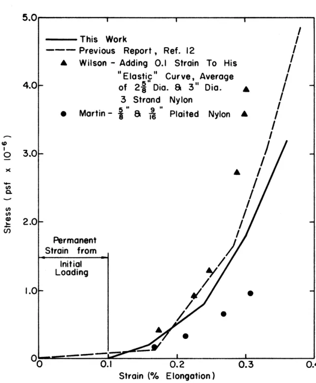
It is very difficult to determine the elongation characteristics for ropes made of synthetic fibers for a general study. Generally, polyester materials have less elongation than nylon for the same stress condition. However, the type of rope, twist-lay, plaited, etc., and the tightness of the strand will influence the load-elongation curves to a great degree, so that it is possible and it has occurred that certain types of nylon ropes will display less elongation than certain types of polyester ropes. Generally, of course, the reverse is true. In addition, the stress-strain charac-teristics are considerably influenced by submersion of the rope, yet practically no information exists on this topic. Thus, a designer has little information to work with unless tests can be performed, under water, on the very rope he plans to use. For this study is was assumed that the mooring rope was subject to an initial and permanent strain of 0.1 from the initial, or some subsequent, loading. The stress-strain diagram is presented in Fig. 3. Also on Fig. 3 are the results of some testing that are reported on in Martin (7) and Wilson

(15) and the stress-strain diagram used in Ref. 12. The final

selection of the stress-strain diagram was somewhat influenced by test information provided by the Columbian Rope Company.

The internal hysteretic damping characteristics for the line were estimated from information given in Refs. 15 and 16. The procedure was to measure the area (thus the energy dissipated ) of several hysteresis loops, approximate them as elipses and utilize the follow-ing equations. For an eliptical hysteresis loop, the amplitude of the loading function Po ' is related to the amplitude of the displacement, Xo ' and the phase shift, B , with:

sin B

=

Area within the elipse

11' P X

o 0

(18)

Thus, B can be determined. Simple linear damping in a continuous system is characterized by

a(s,t)

=

E E(S,t) + Q -

aE

_at

or in a non-linear system (as considered in this report) by a(s,t)

=

aCE) + Q

~

_at

(19)

(20) where a is the stress (calculated as the line tension divided by the original cross-sectional area of the line). E is the modulus of elasticity of the material, E is the strain and Q is the damping coefficient. The damping coefficient, Q , can be estimated by considering the linear system, wherein

(21)

mean, or dynamic modulus of elasticity. Thus 1 . -1 (EliPse area)

Q

= ;;

Ed tan Sln 'If p X

o 0

Thus from Refs. 15 and 16, Q was estimated to be Q

=

4 . 106 w lb - sec ft2 (22) (23)

For the solution of the numerical program the drag forces in the longitudinal direction on the line were ignored. It has been shown in several studies that they have negligible influence when scope is less than 2. The drag coefficient in the radial direction was taken equal to 1.4 and the added mass coefficient was given the theoretical value of 1.0 for a smooth circular cylinder. The saturated mass density of the line was developed as

lJ

=

1.71 02 (24)

where lJ is the mass per foot and D is the line diameter in feet.

Equation 24 was based on a saturated mass density of the line of 2.17 slugs per cubic foot.

A physical description of the buoy is presented in Ref. 12. Several coefficients were derived for the buoy from experimental

information. The drag coefficient in the x2 direction is a function of Froude number, but for the relative velocities considered here it was felt it could be assumed to be constant at 0.035. The added mass

coefficient, CIR ' was 0.4.

In order to obtain similarity between the numerical model and the results of the hydraulic model study reported in Ref. 3 with respect to response decay curves, it was necessary to arbitrarily modify the

usual expression for drag force in the z2 direction of the buoy by making the force proportional to the velocity instead of the velocity squared. In Eq. 10, Fz2 was established for one pie-piece as

Fz2

=

C n(40)2

l-~

V

DA 4 12 2 z2 (25)

Thus the drag coefficient is no longer dimensionless. For this work the value of C_DA was 12.0. The value when the relative acceleration in the z2 direction at the chine was positive of CIA was taken as 3.0, and 0.8 when that relative acceleration was negative. The

auxiliary damping coefficient, q , in Eq. 11 was given the value

200,000 ft-lb-sec. The distance X J was determined to be 9.0. The

dimensional wind drag coefficient, , where W

=

C p . V2/2 Ow a1r w

was determined experimentally in Hath (13) to be 140. The resulting buoy motion due to the above selection of coefficients is given in the next section.

NUMERICAL RESULTS

Longitudinal and Transverse Motion of the Line

One way to check a numerical model such as the one presented here is to compare the results from it to those from a closed solution of a simplified problem. This was done for the case of a taut vibrating string, the solutions of which are well known. The development of the analytical solution will be presented first, followed by compar-isons of analytical results with those from the numerical model.

Consider a straight, weightless line held vertically as shown in Fig. 4. The line has a cross-sectional area of A and a modulus of elasticity of E The initial tension in the line is T

o At

z

=

L the line is forced with a longitudinal excitation, Zo sin wt ,

where w is the radian frequency of the excitation, and it is

assumed that the initial tension is adequate to preserve the condition of positive tension in the line at all locations and times. It is assumed that the effects of damping are negligible. The vertical displacement of a particle of the line will be designated as ~ and the strain in the line is then ~z ' where the subscript indicates the partial derivative with respect to z Only the steady state vibration solution to the problem is desired. It is well known that the governing equation is the wave equation, which is:

(26)

where ~tt is the second derivative of the displacement with respect to time and a turns out to be the celerity of an elastic wave along the line also given by Eq. 2.

The displacement is then a function of the coordinate, z ,and the time, t ,and the boundary conditions are:

z;(o,t)

=

0 (27)

Z;(L,t)

=

Zo sin wt (28)

It should be noted that L »Z and that the problem has been o

linearized by imposing the boundary condition at z

=

L instead of the true condition, z

=

L + Z sin wt

o The solution is obtained by assuming that it is a product in the form:

z;(z,t)

=

(A cos ~ z + B sin ~ z) sin wt

a a (30)

By imposing the first boundary condition it is seen that A

=

0

By imposing the second boundary condition it is seen that B

=

Z / wL o a The solution for the displacement due to dynamic motion is then

z;(z,t)

=

Z

I

.

wz . t L S1n - S1n w o • w a S1n -(31) a and for the strain:

w 1 wz

z;z(z,t)

=

Zo

a .

wL cos

a

sin wt

S1n--(32)

a

MOst ropes do not have linear elastic characteristics, but if they are stressed to at least 20% of their ultimate strength the stress strain diagram becomes approximately linear. The linear condition was assumed for this section of the work.

For a linear elastic material the strain is directly proportional to the stress through the modulus of elasticity, so that the solution for the dynamic line tension, T ,is

T(z, t)

=

_{AE Zo -}w _{a .} 1 _{wL cos -- S1n} wz. _a wt

S1n

-(33) a

For the total tension the steady tension, To ' must be added to Eq. (33). By substituting Eq. 33 into Eqs. 26 through 28 it is seen that it is the solution desired for the steady state vibration

condition.

Equation 33 shows that the line tension has infinite values where . wL 0

S1n -

=

This will occur when a

wL

- =

_a 11 11' n

=

1,2,3, . . •

(The case for n

=

0 is a trivial case where either L

=

0 or

w

=

0)

The numerical model was tested by modifying it to consider a

(34)

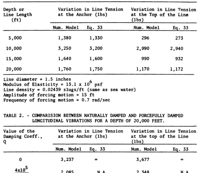
linear elastic material with no damping and with longitudinal motion only. A frequency of 0.7 radians per second was used to represent ocean wave frequencies that can occur as strong swell. Several water depths, or lengths of line, were checked and Table 1 shows the results.

The line tensions were plotted by the computer for the anchor and the buoy end as functions of time. Examples of such plots are shown as Figs. 5 and 6. It was also seen by inspection of the

printed output that nodes of zero tension fluctuation occurred at the positions on the line which are predicted by Eq. 33.

It was attempted to create a resonant condition by selecting a frequency such that wL/A

=

211' The purpose was to investigate the effects of internal damping on preventing infinite response as

predicted by Eq. 33. However, even by setting the damping coefficient,

indicated that the numerical solution as presented was naturally damped. At this writing it has not been determined why the numerical solution as presented here is naturally damped.

It was also discovered that the full amount of damping, as

predicted by Eq. 23, produced a numerical instability in the program. However, when one-tenth of the theoretical value of damping was used, the solution was stable for most conditions and it is felt that this degree of damping in conjunction with the natural damping will produce results that will approximate the action of a real nylon line. The results of testing the solution for a 20,000 feet long line are given in Table 2.

The results show that for the conditions assumed the oscillations in tension were reduced by one-third. For frequencies that were not near the resonant frequencies the damping had little influence on the oscillations, as expected.

The numerical model was also checked in the transverse, or x direction. In this case the steady state transverse vibration was determined for all positions, z , and time, t The analysis assumed that displacements were very small and that the tension in the line was constant in time and position.

The assumed conditions were that both ends of the line remain fixed and at time equal to zero the transverse velocity of the line was sinusoidally distributed along the line. As time progressed the horizontal displacement of the line was also longitudinally distributed and the following development will show the closed solution for the horizontal displacement, n(z,t) The boundary conditions for this problem are,

n(o,t)

=

n(L,t)

=

0 The initial condition is

( ) V . wz

n

_t Z,o

=

0 S1n

b

where Vo is any convenient velocity amplitude and b is the longitudinal celerity of a displacement wave along the line given also by Eq. 3.

The governing equation is again the wave equation,

A product solution is assumed and the general form is

( ) (C w D· w ) . n z,t

=

cos b Z + S1n b Z S1n wt (35) (36) (37) (38)

After applying the boundary conditions and the initial condition, the solution is found to be,

v

w

( t ) o . z . t

n z,

= -

Sl.n 0 S1n w

w (39)

Equation 39 shows that there are nodes on the line of zero displace-ment for all time. In the numerical program the tensions were set to be constant with time and position and all drag and added mass

coefficients were set equal to zero.

For the numerical work, an initial tension of 3905.2 pounds was assumed in addition to a frequency, w , of 0.251 rad/sec and a line length of 20,000 feet. It is seen, then, from Eq. 39 that nodes should occur in the line at z

=

5,000, 10,000, l5,OOO,and 20,000 feet. The results of the numerical work showed that the nodes

occurred at about z equal to 5400, 10,000, 15,400 and, of course, 20,000 feet.

The maximum magnitudes of the displacements should be 18.3 feet, as predicted by Eq. 39. Figure 7 shows that the displacements were not perfectly symmetrical, mostly due to the fact that the nodes did not occur exactly where they were supposed to occur. However, the average maximum displacement as determined from Fig. 7 is 18.3 feet.

The conclusion from the above tests was that the rating of the numerical model can be described as from good to excellent, the first rating applied to the transverse motion and the second referring to the longitudinal motion.

Many buoy moorings are established with a very taut line running almost vertically from the anchor to the buoy. It will be shown below that the resonant length or frequency of the mooring line will depend a great deal on the type of buoy that is used at the water surface.

One condition for consideration is that shown by Fig. 4 where the longitudinal displacement at the top of the line is imposed as the boundary condition. The equation of motion in terms of displace-ment is given by Eq. 31 and the line tension is given by Eq. 33. These equations show that resonant conditions exist when wL/a

=

nn

Consider next equal conditions except that the boundary condition at the top of the line is a force given by

f L _z=

=

F sin wt ₀ (40)

The new boundary conditions, for a material with a linear stress-strain relationship, are given by Eq. 40 and

~

(L,t)

= 1-

F sin wt

z AE 0

On substitution of the boundary conditions into Eq. 30, one again finds that A

=

0 and that

thus,

B - cos -w _a (&)L. _a S1n (&)t

= -

1 F S1n (&) . t

AE 0 F B - 0 a __ l~~ - AE

w

wL cos -a

and the solution for displacements is, F ( ) 0 a 1 . (&)Z . t ~ Z, t

= - -

L S1n - S1n (&) AE w w a cos -_a (41) (42) (43) (44)

The curious difference between Eqs. 44 and 32, is that infinite responses occur for Eq. 32 at (&)L/a

=

nw but for Eq. 44 they occur at

w

wL/a

=

n

'2 •

For design purposes the resonant conditions should be avoided. For very taut moorings that approximate the configuration shown in Fig. 4 the most serious mode of motion will probably be the longitudi-nal one. Damping may be relatively low. The resonant length of line, given a particular wave frequency, will then depend on the boundary condition at the top of the line.

Consider two types of buoys that may conceivably be moored to nearly vertical mooring lines at the air-water interface. One buoy is a surface following large disc and the other is a non surface, or relatively stable, spar. For a flexible mooring line the large disc will impose a displacement at the upper end of the line as it closely

follows the undulations of the water surface whereas the spar buoy will impose a time varying force on the line as the waves pass the spar. For a particular wave frequency the resonant length of line for the disc mooring will be

L=n.!!.

00 n

=

1, 2, 2, • • •

For the spar buoy, the resonant length of mooring line will be 1I'a

L

=

n 200 n

=

1, 3, 5,

(45)

(46)

For other buoy types, such as the aid to navigation buoys used by the U. S. Coast Guard, some condition between Eqs. 45 and 46 will exist. In addition, several wave frequencies exist at sea and all resonant conditions with respect to the entire wave frequency spectrum should be investigated.

To illustrate with numbers the foregoing concepts, consider a common ocean wave period of seven seconds. The frequency will be 0.90 radians per second. Assume that a one-inch diameter nylon line

(that is nearly neutrally buoyant) is used and that it is pre-stressed to 2200 pounds. The modulus of elasticity will be about 7.5 x 106 psf according to Fig. 3. The saturated density of the line will be about 0.0118 slugs per foot. Thus the celerity of a longitudinal elastic wave in the line will be about,

or, a

=

.00547 x 7.5 x 10 6 0.0118 a

=

1860 fps (47) (48)

For the disc buoy, the resonant lengths of mooring line will be 6,500 feet, 13,000 feet, etc. For the spar buoy, the resonant lengths of line will be 3,250 feet, 9,750 feet, etc. It should be stated again for emphasis that all wave frequencies should be examined for the resonant lengths of the line and the type of buoy must be given careful consideration.

Now consider the equations for line tension for both the above conditions. For the disc buoy the tension is given by Eq. 33. For the spar buoy the tension will be,

T(z,t)

=

F 0 1 wL cos -- S1n wz. wt

cos __ a (49)

a

For both conditions the dynamic line tension is a maximum at the

anchor! For the disc buoy the dynamic tension at the buoy may be zero if wL/a

=

nn/2 with n

=

1,3,5,

line tension at the buoy will be

For the spar buoy the dynamic F sin wt

o and the displacement will be zero if wL/a

=

nn n

=

1,2, •.•

Buoy Motion

A necessary part of this study was to select the proper values of the coefficients in Eqs. 9 through 17. The procedure was to rely heavily on the 1:10 scale model study in Ref. 3. In particular some response decay curves for the pitch and heave motions were generated that implicitly display the effects of all the coefficients. By trial and error the coefficients were evaluated for the numerical model until the predicted response curves nearly matched the best estimate for the response curves of the prototype. The response curves for the prototype were estimated from the response curves from the scale

model study by considering the Froude modeling relationships and the shift in natural periods due to different degrees of damping.

Hydrodynamic damping in the model studies should be greater than in the prototype because of the Reynolds number scale effect. The

natural period in heave for the prototype predicted by the model study was about 3.6 seconds. After accounting for the Reynolds number

effect, the period was reduced to 3.2 seconds. The period in heave from the numerical model was 3.1 seconds, which was considered to be close enough. Peaks in tension spectra from prototype measurements occur at periods of from 3.1 to 3.4 seconds and it is predicted here that they were due to the heaving motion of the buoy. The model study also showed a ratio of 1.128 between the heave period and the pitch period. The ratio for the numerical work is 1.148.

Figure 8 presents the normalized pitch response decay curve for the numerical work and the results from the hydraulic model study where the normalizing pitch is the pitch at time equal to zero and the normalizing time is the natural period. A similar curve is presented in Fig. 9 for the heave motion; however, the beginning portion of the data from the hydraulic study appeared to be influenced by the release of the buoy model at the start of testing. Thus the curve for the hydraulic model was arbitrarily shifted to the left so that the subsequent vibration would be in phase with those from the numerical work.

One minor but interesting phase of this work was to observe the predicted motion of the buoy on the surface of a wave. For this part of the work it was assumed that the buoy was moored in 200 feet of water with an elastic material that produced an equivalent spring

constant at the buoy of 10 lbs/ft, always directed toward the anchor,

with an initial tension of 50,000 lbs. As in all the work involving

waves, the wave height was built up linearly with respect to time over

one wave period. Thus Fig. 10 shows how the wave height was increased

over the first wave period and how the buoy and mooring behaved for a

wave 260 feet long and 36 feet high. For this case the mass-spring

system in conjunction with the water particle acceleration was such

that the attachment point was exposed to the air shortly after 14

seconds and the program was written to stop for such an occurrence.

Figure 11 shows the buoy successfully negotiating the same wave for

the free-floating condition and Fig. 12 shows a successful transit

of the moored condition when the wave height was reduced to 30 feet.

A much longer and higher wave is presented in Fig. 13. Figure 13

clearly shows the buoy heaving on the wave at the natural damped

period of 3.1 seconds, as well as at the period of the wave.

Water Sheave

Another minor but very interesting investigation made during this

study was that which is sometimes referred to as the "water sheave"

effect. An illustration of the problem is, say, a mooring in 20,000

feet of water subjected to a ISO kt. wind. At some time the wind

suddenly shifts 1800 and blows the buoy back along the alignment of

the mooring line until it and the line reach new equilibrium positions.

How the line tension varies during the transient motion has been in

question. It is felt that the form of the line tension solution

presented here, based on the method of characteristics, is particularly

A similar problem as that posed above was investigated. However, in order to save computer time the top of the line was translated at a higher velocity than would be the case if the wind drag only on the buoy were reversed. First it was determined that if the buoy broke

free from the mooring, alSO kt. wind would push it through the water with a speed of 13 ips. It was decided to translate the line at the

conservatively much higher velocity of 25 ips, increasing it linearly from 0 ips in the period of 20 seconds.

An

initial "in place" or tensioned scope of about 1.3 was assumed and the initial

non-equilibrium tension of 7000 lbs. was established with a line diameter of 1.5 inches for a material with characteristics as shown in Fig. 3. The first computation consisted of fixing the top of the line in place and allowing it to reach an equilibrium position. Both positions are shown at time equal to zero on Fig. 14. Then the line was moved to the left with the velocity function presented above. The sequential positions of the line as determined by the numerical computations are shown in Fig. 14.

The tension in the line dropped during the first 150 seconds and then gradually increased until nearly rupturing the line, at which time the computations were stopped. During the increase in tension phase the maximum tension occurred at about 0.067 the distance down the line. The line length changed in accordance with the state of tension along the line. The tension contours on the s-t plane are shown in Fig. 15. It should be noted when examining Fig. 15 that station 1 represents the anchor and subsequent station numbers are spaced 866.7 feet apart. It can be seen that the tension at the anchor decreased for about the first 150 seconds and then steadily

increased. Toward the end of the computations the tension in the line was nearly constant with respect to line position, which is reasonable by inspection of Fig. 14.

If the top boundary condition had been the actual buoy with the wind only driving it, the tensions would have been lower because of the

lower buoy velocity and because of the differences in the initial loading condition. When the horizontal component of the line tension at the buoy had equaled the wind drag of 10,800 pounds the buoy-motion would stop. Thus it can be seen that the conditions imposed were much more severe than what would have been experienced at sea. If the submerged weight of the anchor were less than about 10,000 pounds it would have been lifted from the bottom (assuming no adhesion to the bottom) at around 1000 seconds or more. If the real boundary condition had been imposed at the buoy end, the motion would have been quite slow and the computer time necessary to complete the problem would have been prohibitive within the budget for this study.

Effects From the Environment at Sea

The main purpose of this research was two-fold; 1.) to complete the debugging of the numerical program and to test it against closed mathematical solutions, as already discussed, and 2.) to gain some insight into the influence on dynamic line tensions from different wind and current loads and different line scopes. The work related to the first item has been presented. For the second purpose it was decided to design a few moorings in 20,000 feet of water for certain scopes for a maximum wind condition of 150 kts., subjecting each mooring to waves of various frequencies. Then the same moorings were tested with the same waves but with a moderate wind velocity of 50 kts.

The current velocity profiles corresponding to the two wind velocities are presented in Fig. 2.

As presented previously, the computer program first determined the steady state, or equilibrium, position of the lines. The five different conditions are shown in Fig. 16. In all cases the equilib-rium tension in the line was kept below 47% of the breaking strength as predicted by Fig. 3. Thus three diameters were selected, as shown in Fig. 16. A summary of the load and scope conditions is given in Table 3.

Two short runs were made in shallow water in order to obtain a brief view of the influence of fairly large waves on line tension. The steady load conditions for these two runs are summarized in Table 3. The profile equilibrium positions have not been included in a Figure because they were practically straight lines.

The dynamic program based on the method of characteristics was compared to the steady state program in terms of the static loads. The procedure was to assume a water depth of 10,100 feet, a scope of

2.02, diameter of 3 inches, a 100 kt. wind, no wave and a surface current of 6 kts. As before, the steady state program determined the equilibrium conditions, which established the initial conditions for the dynamic program The dynamic program was then allowed to run to a real time of 6S seconds during which no environmental conditions were changed. The configuration of the line changed somewhat, but not beyond what was felt were acceptable limits. It was found that the angle at the top of the line decreased (which was anticipated because of the change from equal angle increments to equal distance increments along the line) as well as the angle at the bottom of the line. The

program ran until the angle at the top decreased to a mimimum value, and then was increasing to when the computations were stopped. The line tensions were re-distributed somewhat but the total line length and the buoy coordinates changed very little. A summary of the computations is given in Table S.

It was next desired to subject the five mooring conditions to waves of various frequencies, or lengths. In each case the wave

height to length ratio was kept constant at 1:15. Thus the waves were not nearly breaking but also they could not be classified as small amplitude waves. The dynamic tensions at various stations along the line were determined and plotted by the computer. Generally, the maximum dynamic tensions occurred at the buoy or at the anchor. Examples of tensions at the buoy and at the anchor are presented as Figs. 17 through 32. Point 31A refers to the attachment point at the buoy_ It will be noticed that other frequencies, in addition to the

frequency of the imposed wave, are present. All periods of frequencies in evidence will be accounted for later.

The computer outpup included tension contours in the s-t plane. Examples are shown for conditions I through V for the 500 feet long wave as Figs. 33 through 37. The value of each contour line has not been indicated but can be determined by the reader by referring to Figs. 17 through 32. The important thing in Figs. 33 through 37 is to notice the pattern of line tensions. The nodes of zero or small tension fluctuations are clearly visible, as are the regions of

maximum tension fluctuations. Equations 33 or 49 can also be used to approximate the locations of the nodes if the z is replaced with s That is, the nodes occur where cos ws/a

=

o.

A comparison of the

results obtained from the numerical model with those from Eqs. 33 and 49 is presented in Table 6. The comparison is fairly good except at the highest wave frequencies. Thus the position of the nodes can be estimated from Eq. 33, regardless of the line curvature. This introduces the possibility of determining the best position for locat-ing sensitive instrumentation, at least with respect to line position. That is, the positions of minimum displacement variation can be

determined from Eqs. 31 and 44 by setting S1n -. (Us

=

0 a

minimum tension variation can be determined by setting

, or the (Us

cos - = 0 or a

the minimum line velocities can be determined from a contour map of velocities or by taking the total time derivatives of Eq. 31 or 44.

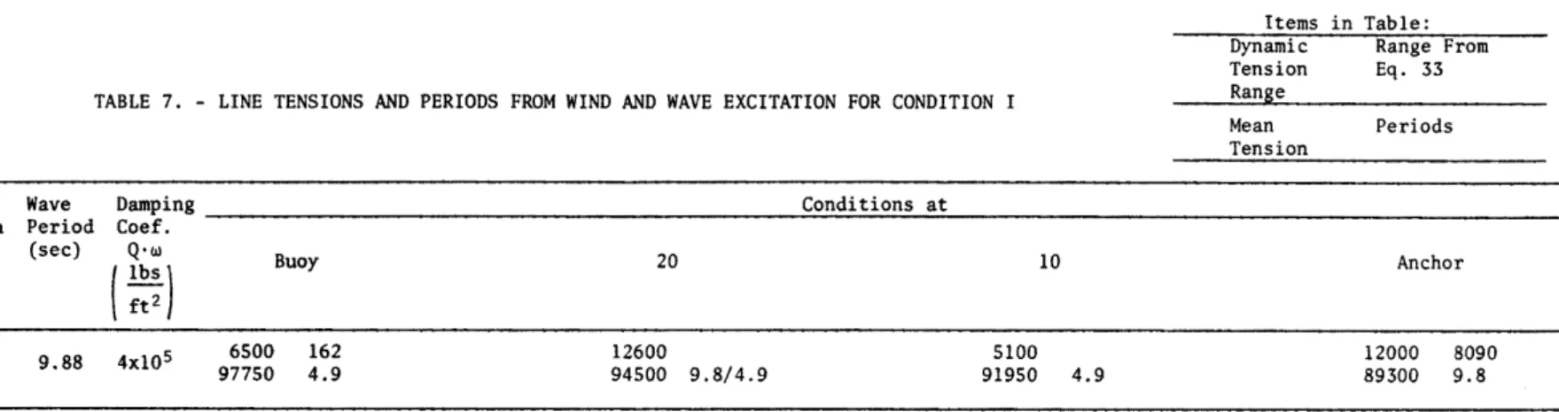
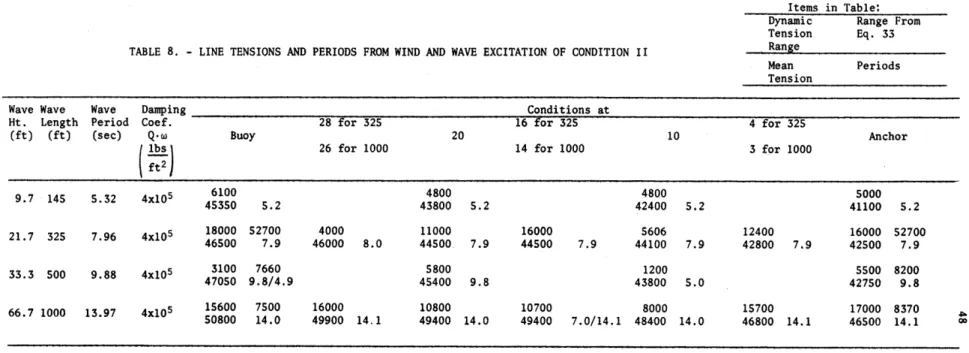
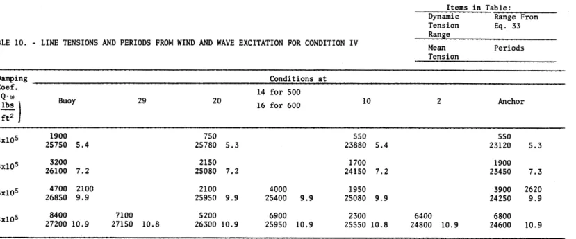
A complete summary of the runs made with waves for conditions I through V is given in Tables 7 through 11. Included in the Tables is the value of the damping coefficient, Q , used, the range, or double amplitude, of dynamic tension, the mean value of line tensions at the end of the run, the periods of the frequencies evident in the output records and a calculated line tension based on Eq. 33 for which the length of the line was taken as the "stretched" or "in-place" length at time equal to zero, and the modulus of elasticity was taken as that corresponding to the tension in the top of the line at time equal to zero.

It is desirable to be able to display and compare mooring line tensions in a way that takes into account the difference in line diameter and length, the differences in wave height and frequency and the resonant frequencies. Thus it is desirable to normalize the tensions and corresponding frequencies to compare the results of different types of moorings. The normalizing factor for tensions for

this study was based on the total saturated mass of the line

(excluding the added mass) and a characteristic wave acceleration. Thus

Normalizing force

=

p L H W2

Since eq. 33 can predict the nodes in the line fairly well for the moorings presented here, it was felt that Eq. 34 may suffice for predicting, at least approximately, the resonant frequencies with

(SO)

regard to line tensions despite the presence of considerable curvature in the line. Thus the first modal frequency predicted by Eq. 34 was used as the normalizing frequency. Conveniently, the first resonant condition should occur at flfl

=

1.0 and the subsequent higher mode resonant conditions occur at f/fl

=

2.0, 3.0, 4.0, etc. The resonant frequencies of interest for the five conditions are presented in

Table 12. The resulting normalized frequency response curves for conditions I through V are presented as Fig. 38 for mooring line

tension at the buoy and Fig. 39 for mooring line tension at the anchor. Admittedly, the data is sparse, but the trend for moorings considered here is clear. That is, the greatest dynamic response, especially at the resonant conditions, occurs for the higher wind conditions. The next most influential parameter is the line scope. It has already been seen, and is common knowledge, that scope is a most important parameter for steady state loads. The responses at higher frequencies tend to be damped out due to hydrodynamic action. No data was

obtained for flf _n

=

1.0 because such a condition would be due to waves considerably longer than 1000 feet and such long waves were uneconomical to consider. However, little energy exists for waves longer than 1500 to 2000 feet in most wave spectra.

With several curves like Figs. 38 and 39 for a complete range of water depths, scopes, line diameters and types, it may be possible to generate a non-dimensional empirical solution for dynamic line tensions for any homogeneous one point mooring. Or perhaps analytical transfer functions based on linear systems, which are being developed by others, can be compared to results like Figs. 38 and 39, which consider most of the non-linearities in the problem. This subject has been left for future study.

In order to test the program for quite shallow water conditions and to gain whatever information possible with just two runs, condition VI for a depth of 150 feet and condition VII for a depth of 1000 feet were investigated for a wave 600 feet long and 40 feet high.

For the depth of ISO feet the sequential positions of the line are shown in Fig. 40 from time zero to 13 seconds. At about time equal to 14 seconds the line tension became negative and the program stopped because a square root of the negative tension occurs. The line tension, which was nearly constant along the line at any time is shown in Fig. 41.

For the depth of 1000 feet the line remained nearly straight for all motion. The line tensions again were nearly constant along the line at any time. The fluctuations in the tension at the buoy and at the anchor are shown in Fig. 42. It should be recalled for both conditions VI and VII that the wind velocity was SO kts.

SUMMARY AND CONSLUSIONS

A review of the basic equations for the numerical modeling of the mooring line motion based on the method of characteristics and the motion of the buoy has been made. Solutions for a homogeneous mooring line have been presented which include hysteretic damping and hydro-dynamic damping. In addition, a summary of analytical solutions for a straight, taut mooring line has been presented and it was attempted to apply the procedures developed to the single point curved, or less taut, moorings. It was found that this approximate procedure did poorly for estimating mooring line tension but did quite well in

estimating the positions of the nodes of tension and in predicting the natural resonant frequencies of the line.

A new way of presenting frequency response curves for taut or slack mooring lines subjected to waves was suggested. The normalizing procedure makes it possible to show the frequency response for lines of different lengths, diameters and materials on the same scale. Thus the influence of scope and wind magnitude on dynamic mooring line

tension was presented while normalizing the influence of line diameter. It was found that smaller scope and/or higher wind increased the

dynamic tensions drastically, as well as the steady state, or mean line tension.

Two runs were presented for shallow water. It was seen that a large wave in ISO feet of water would have been disastrous to a 2 inch diameter line. However, the same wave in 1000 feet of water with the same line and scope produced reasonable dynamic tensions. It was seen that the tension was nearly constant along the line at any time.

Probably a static solution approach would be adequate wherein the line tension would be determined based on the sequential positions of the buoy on the wave and the subsequent change in scope without regard to accelerations. However, this procedure would be very inade-quate for deep water moorings.

A presentation of the water sheave problem was made which illustrated an additional application for the numerical program.

REFERENCES

1. Berteaux, H. 0., "Design of Deep Sea Mooring Lines," Marine Technology Society Journal, Vol. 4, NO.3, May-June, 1970. 2. Devereux, R., et.al., "Development of An Ocean Data Station

Telemetering Buoy," Progress Report GDC-66-093, Convair Division of General Dynamics, December, 1966.

3. Felix, M. P., "Hydrodynamic Drag and Frequency Response Characteristics of a Model of a Large Oceanographic Buoy," Internal Report GDC-ERR-139l, Convair Division of General Dynamics, December, 1969.

4. Fofonoff, N. P., and Garrett, J., "Morring Motion." Technical Report Reference No. 68-31, Woods Hole Oceanographic Institute, May, 1968.

s.

Froidevaux, M. R., and Scholten, R. A., "Calculation of the Gravity Fall Motion of a Mooring System," Report E-23l9,

Instrumentation Laboratory, Massachusetts Institute of Technology, August, 1968.

6. Goeller, J. E., and Laura, P. A., "Analytical and Experimental Study of the Dynamic Response of Cable Systems," Report 70-3

Institute of Ocean Science and Engineering, The Catholic University of America, April, 1970.

7. Martin, W. D., "Tension and Geometry of Single Point Moored Surface Buoy Systems. A Computer Program Study," Technical Report Reference No. 68-79, Woods Hole Oceanographic Institute, December, 1968.

8. Mercier, J. A., "Hydrodynami c Forces on Some Float Forms,"

Report SIT-DL-69-l407, Davidson Laboratory, Stevens Institute of Technology, October, 1969.

9. Millard, R. C., "Observations of Static and Dynamic Tension Variations from Surface Moorings,tt Technical Report Reference No. 69-29, Woods Hole Oceanographic Institution, May, 1969. 10. Nath, J. H., and Felix, M. P., MA Report on a Study of the Hull

and Mooring Line Dynamics for the Convair Ocean Data Station Telemetering Buoy," Internal Report GDC-ERR-AN-ll08, Convair Division of General Dynamics, December 1, 1967.

11. Nath, J. H., and Felix, M. P., "A Nwnerical Model to Simulate Buoy and Mooring Line Motion in the Ocean Environment," Internal Report GDC-AAX68-007, Convair Division of General Dynamics, August 22, 1968.

12. Nath, J. H., "Dynamics of Single Point Ocean Moorings of a Buoy-A Numerical Model for Solution by Computer," Progress Report Reference 69-10, Department of Oceanography, Oregon State University, July, 1969.

13. Nath, J. H., "An Experimental Study of Wind Forces on Offshore Structures," Technical Report CER70-71JHN3, Department of Civil Engineering, Colorado State University, August, 1970.

14. Paquette. R. G., and Henderson, B. E., "The Dynamics of Simple Deep-Sea Buoy Moorings," Technical Report 65-79 Nonr-4558(00) to Office of Naval Research, General Motors Defense Research Laboratories, Santa Barbara. California, November, 1965. 15. Schram, J. W., and Reyle, S. P., "A Three-Dimensional Dynamic

Analysis of a Towed System," Journal of Hydronautics, Vol. 2, No.4, October, 1968.

16. Wilson, B. W., "Elastic Characteristics of Moorings," Journal of the Water Ways and Harbors Division, American Society of civil Engineers, Proceedings paper 5565, November, 1969.