Multi-Agent-Based Simulation for Analysis of Transport
Policy and Infrastructure Measures
Johan Holmgren1, Linda Ramstedt2, Paul Davidsson3, and Jan A. Persson3 1School of Computing, Blekinge Institute of Technology, SE-374 24 Karlshamn, Sweden
johan.holmgren@bth.se
2Vectura, Svetsarvägen 24, SE-171 11 Solna, Sweden linda.ramstedt@vectura.se
3School of Technology, Malmö University, SE-205 06 Malmö, Sweden {paul.davidsson,jan.a.persson}@mah.se
Abstract. In this paper we elaborate on the usage of multi-agent-based
simula-tion (MABS) for quantitative impact assessment of transport policy and infras-tructure measures. We provide a general discussion on how to use MABS for freight transport analysis, focusing on issues related to input data management, validation and verification, calibration, output data analysis, and generalization of results. The discussion is built around an agent-based transport chain simulation tool called TAPAS (Transportation And Production Agent-based Simulator) and a simulation study concerning a transport chain around the Southern Baltic Sea.
Keywords: Multi-agent-based simulation, MABS, Multi-agent systems, Supply chain
simulation, Freight transportation, Transport policy assessment.
1
Introduction
Freight transportation causes different types of positive and negative effects on the so-ciety. Positive effects typically relate to economy and social welfare, e.g., due to the possibility to consume products that have been produced far away. Negative effects mainly relate to the environment, and typical examples are emissions, congestion and energy use. Public authorities in the role of policy makers often have a wish to reach cer-tain governmental goals, such as obcer-taining suscer-tainable transport systems and meeting emission targets. A typical ambition of a public authority is to increase the internaliza-tion of external costs, e.g., by letting road users pay for the road wear they cause [1]. However, internalization of external costs may have effects that might be negative on other goals. For instance, it might lead to negative economic development in a region. For enterprises, the goal is typically to maximize profit, e.g., through optimization of their activities (either individually or in collaboration), by reducing lead-times, lowering transport costs, improving delivery accuracy, etc.
By applying different types of transport policy and infrastructure measures, here-after referred to as transport measures, it is often possible for public authorities and corporate decision makers to influence how transports are carried out. However, it is important to be able to accurately predict what the consequences will be when applying
This is an Author's Accepted Manuscript of a conference abstract in Lecture Notes in Computer Science, Vol. 7580, (2012) p. 1-15, http://dx.doi.org/10.1007/978-3-642-35612-4_1
Springer©, the final publication is available at: www.springerlink.com (Access to the published version may require subscription)
transport measures, so that undesired effects can be avoided and desired effects can be confirmed. Essentially, there are three types of transport measures that are relevant to apply to a transport system:
1. Control policies including different types of taxes and fees, such as kilometer and fuel taxes, and regulations, such as weight restrictions on vehicles.
2. Infrastructure investments in roads, railway tracks, intermodal freight terminals, industry tracks, etc.
3. Strategic business measures, such as improvement of timetables and adjustment of vehicle fleets to better meet the transport demand.
Multi-agent-based simulation (MABS) is able to model the actual complexity of a transport system, e.g., by explicitly modeling decisions of different actors (e.g., trans-port operators and transtrans-port buyers), their interaction, time aspects (including timeta-bles and time-differentiated taxes and fees), etc. This is necessary to get accurate results when assessing the impact of transport measures, and it makes MABS more powerful than traditional approaches to transport analysis, such as SAMGODS [19, 3], SMILE [20] and TRANS-TOOLS [15]. Whereas traditional approaches rely on assumed statis-tical correlation between different parameters, MABS relies on causality, i.e., decisions and negotiations determine how transport activities are performed. Since MABS is able to capture the interaction between actors, as well as their heterogeneity and decision making, it enables more explicit modeling of the complex multi-actor processes in-volved in finding and agreeing upon transport solutions. Typical questions that can be studied using MABS models for impact assessment of transport measures include:
– Which logistical effects (e.g., concerning transport route/mode choices, order sizes
and order frequencies) will appear in a particular transport network under the influ-ence of a set of transport measures.
– How will the costs and quality of service (e.g., possible delays) change as a
conse-quence of the introduction of a set of transport measures.
– What will the environmental impact (e.g., CO2 emissions) be when introducing a set of transport measures?
The purpose of this paper is to elaborate on the usage of MABS for impact assess-ment of transport policy and infrastructure measures (transport measures). We build our discussion around experiences that we have gained when developing and using an agent-based simulation tool called TAPAS (Transportation And Production Agent-based Simulator) [2]. We briefly describe TAPAS, as well as a simulation study that has been conducted with TAPAS. The simulation study concerns transportation in a transport corridor around the Southern Baltic Sea.
In our work we focus on the TAPAS simulation tool even though there exist several other MABS models that can be used for assessing the impact of different types of trans-port measures, e.g., provided by Gambardella et al. [6] and Liedtke [14]. We assume that they in most aspects concerning how to conduct simulation studies are similar, even though they are different in many other aspects.
By presenting and accounting for how to conduct a MABS study for impact assess-ment of transport measures, we contribute with respect to determining the purpose of
a study, designing simulation experiments, validating scenarios, and analyzing simu-lation results including the possibility of obtaining generalizable results. Particular as-pects that are addressed in the discussion are our experiences concerning participatory and collaborative modeling and simulation, how to select which entities and aspects to include in a simulation study, and how multi-criteria analysis with MABS can be used when analyzing the impact of transport measures, e.g., to assess whether measures are good enough from a sustainability perspective. We believe that our work may be valu-able when developing new MABS models for impact assessment of transport measures, and when designing and conducting simulation studies using existing models.
In the next section we give an overview of TAPAS, followed in Section 3 by a de-scription of a simulation study that has been conducted with TAPAS. Section 4 contains our main contribution, which is a discussion on how to design and conduct simulation studies with MABS models, and in Section 5 we provide some concluding remarks.
2
The TAPAS simulation tool
We here briefly describe the TAPAS simulation model, which is an agent-based tool for simulation of decision making and activities in transport chains. The main purpose of TAPAS is to function as a decision support system for different types of users and stakeholders by allowing them to study different types of transport measures. A detailed description of TAPAS, including technical details, is provided in [8].
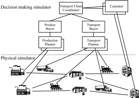
As illustrated in Fig. 1, TAPAS makes use of a 2-tier architecture including a physi-cal simulator and a decision making simulator. The physiphysi-cal simulator models all phys-ical entities (e.g., links, vehicles, and products) and their activities, and in the decision making simulator, six transport chain decision makers (or roles) are modeled as agents.
2.1 Decision makers and their interaction
To fulfill a customer demand, the agents participate in a process that includes ordering of products and a transport solution, selection of which resources and infrastructure to use, and planning of how to use resources and infrastructure. The process starts when a customer sends an order request to the transport chain coordinator, and it ends when products and a transport plan have been booked and confirmed.
The customer is responsible for ordering products in quantities that keep customer inventories at levels that minimize the costs for inventory holding and ordering (order cost includes costs for production and transportation) while reducing the risk of run-ning out of stock. The transport chain coordinator is responsible for fulfilling customer orders by requesting products from the product buyer and transport solutions from the transport buyer. For a number of candidate order quantities, it finds the best combi-nation of products and transportation and lets the customer determine which quantity should be delivered. The product buyer is responsible for finding products in order to satisfy product requests (from the transport chain coordinator), and it communicates with the production planners by sending product requests and receiving product pro-posals. A production planner is responsible for planning the production in a producer node, based on available production resources and costs. Production costs and times
Fig. 1. Architectural overview of the TAPAS simulation model.
when products can be picked-up are sent to the production buyer as a response to a product request, and production planners are also responsible for sending bookings to the factories. The transport buyer is responsible for combining transport proposals that are received from the transport planners into producer-to-customer transport solutions. Each transport planner controls a fleet of vehicles, which operates in some geograph-ical area. From transport requests that are received from the transport buyer it creates and returns transport proposals.
2.2 Input and physical entities
In addition to providing some general input, such as length and precision of simulated time, all modeled entities need to be specified in a sufficient level of detail. We will here describe the different types of entities that can be modeled in TAPAS.
Transportation. The transport network is defined as a set of nodes, i.e., customer nodes,
producer (factory) nodes, and connection points (terminals), and a set of directed links, representing connections between nodes. A link represents exactly one transport mode (e.g., road, rail, or sea), which means that more than one link may connect two nodes. A link has a length and an average traveling speed, which defines the traveling speed for vehicles that do not operate according to timetables. The traveling speed of a vehicle that operates according to a timetable is determined by the timetable. For each termi-nal, the analyst needs to specify vehicle-specific fixed costs for visiting the termitermi-nal, how much time it will take to prepare vehicles for loading and unloading, how much
time is required for loading and unloading one unit of each type of product, as well as time-based costs for loading and unloading. Vehicle types are used to specify the char-acteristics of vehicles, and a vehicle type is described by a vehicle weight, maximum allowed weight (including load), load capacity (i.e., a set of storages with capacities), fuel (or energy) type, distance-based fuel consumption, emissions (e.g., CO2and NOx) per unit of consumed fuel, and transport mode. A fuel type (e.g., diesel or electricity) is defined by a cost and a tax that is charged per unit (e.g., liter or kWh). Four types of transport cost components can be defined; time-based costs (e.g., driver and deteri-oration of products), distance-based costs (e.g., fuel, vehicle wear, and kilometer tax), link-based costs (e.g., road tolls), and fixed operator-based ordering costs (e.g., adminis-tration). TAPAS provides two approaches for determining the price for buying transport capacity. In one approach, the price depends linearly on the size of the order, based on assumed average load utilization for the particular type of transport. In the other approach, a risk cost is added to cover for uncertainties regarding future bookings.
Storage. Storages are defined for vehicles, and for customer and producer nodes. A
storage type is described by the types of products that can be stored, and whether or not multiple product types can be stored simultaneously. For example, it might be possible to store more than one type of liquid in the same tank, but not at the same time. A storage is described by a storage type, additional restrictions regarding which product types can be stored (other than specified for the particular storage type), as well as capacity (weight and volume). Moreover, it is possible to specify time-based costs for storing products, which are differentiated on product type and storage owner.
Production and consumption. A product type is described by mass and volume
at-tributes, and for each product type that can be produced in a producer node, the follow-ing parameters should be specified: cost for raw material (for the particular node), max-imum batch size, batch production time, batch setup time, and time-based production cost. The price for products is the cost for raw material plus the production cost, which is proportional to the production time. Even though batch production is assumed, the parameters that describe production can be adjusted to represent: (1) batch production, (2) continuous production, and (3) instant retrieval of products from storage (however without considering inventory costs for the products). Moreover, for each type of prod-uct that can be consumed in a customer node, the analyst needs to define several types of parameters describing the ordering behavior, e.g., maximum allowed inventory level, safety-stock level, and estimated (approximate) order-to-delivery lead time.
3
An EastWest Transport Corridor (EWTC) scenario
In a scenario around the Southern Baltic Sea we studied three types of transport mea-sures aimed at achieving a modal shift from road to rail and sea transportation, which is an explicit goal within the European Union [4]. We studied a kilometer tax for heavy trucks in Sweden, a CO2 tax for all transports in the studied area, and a new direct railway link between Karlshamn and Älmhult (the so-called SouthEast Link). Possible consequences are changes in mode and route choices, transport costs, emissions, etc.
The studied kilometer tax level is suggested by the Swedish Institute for Communica-tion Analysis (SIKA) [5] and it is differentiated based on the euro class and on the total weight of trucks. We investigated a range of CO2tax levels, which are in line with the levels discussed in another report by SIKA [18]. The SouthEast Link is an infrastruc-ture project that is currently discussed in Sweden, and in the study we investigated two different timetables for the considered link.
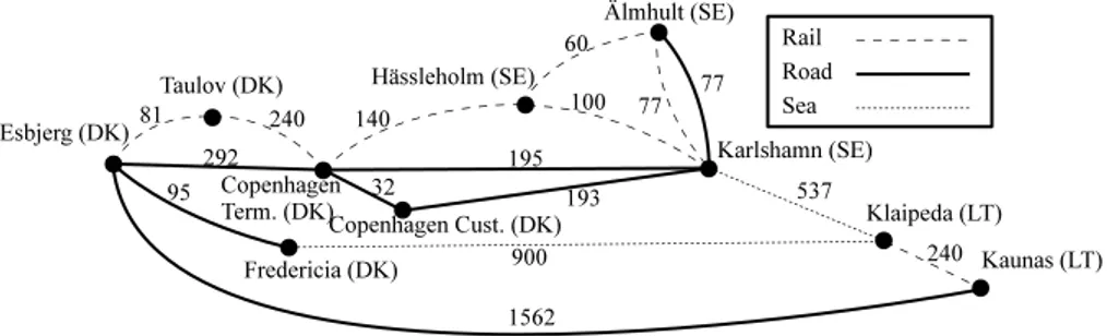
The presented scenario, which is illustrated in Fig. 2, is an extension of a scenario that has been studied earlier in collaboration with partners in a project financed by the EU (http://www.eastwesttc.org). It contains one logistical terminal in Kaunas (Lithua-nia), which provides two types of products, and three typical customers in the studied area; one in Sweden (Älmhult) and two in Denmark (Copenhagen and Esbjerg). In the scenario, transport by rail, road, and sea is offered by five transport providers, and there are several possible routes for transporting 20 ft ISO-containers (TEUs) from Kaunas to the three customers. In the scenario, transportation by sea and rail is assumed to follow timetables while transportation by road is demand driven. A detailed description of the scenario, including input parameters for all entities, timetables, etc., is provided in [7].
Fig. 2. Illustration of the transport network modeled in the studied scenario, where the numbers
on the links represent distances in kilometers.
The input data used in the scenario has been collected from different sources (e.g., http://www.ntm.a.se/). Since the aim was to mirror a real-world scenario, we have used data from existing companies in the studied region as much as possible. However, since the case study models future scenarios, it has not always been possible to make use of real data. Therefore, it was necessary to make certain assumptions, e.g., concerning train frequencies on the SouthEast Link, consumption, customer behavior, and average load utilization for different types of transports. The behaviors of the decision makers are restricted to how they are internally modeled, and they have to communicate with each other according to the interaction protocol in TAPAS. In particular, for the customer we made assumptions regarding order quantities, delivery time windows, safety-stock levels and inventory holding costs.
The scenario and its results have been validated through interviews with domain experts, and a visualization of the scenario helped us discover unrealistic assumptions
and to facilitate the communication of assumptions and simulation results. We have per-formed sensitivity analyses regarding different input parameters in order to understand how different parameters influence the results. In the sensitivity analysis we mainly analyzed load utilization factors of different vehicles and storage interest rates, for im-proved understanding and for calibration of the scenario. As part of the study we also studied different levels of a CO2 tax to analyze how different tax levels may influence the transport system. Moreover, the estimated transport cost structures, i.e., the relations between time-based and distance-based costs have been compared to the cost structures used in the SAMGODS model [19].
In the simulation study we considered the following experimental settings:
S0. The base case refers to the current situation without any of the studied measures. S1. S0 + a kilometer tax of 0.15 euro/km for trucks operating in Sweden, and between
Copenhagen Terminal and Copenhagen Customer.
S2. S0 + a CO2tax for all vehicles operating in the modeled region. Tax levels from 0.10 euro/kg up to 0.30 euro/kg in steps of 0.05 were considered. We let S2.x refer
to setting S2 with a CO2tax level of 0.x euro/kg.
S3. S0 + a new railway link between Karlshamn and Älmhult (i.e., the SouthEast Link).
Two timetables, which are synchronized in different ways with ferry arrivals in Karlshamn (from Klaipeda), were considered: a) worse synchronization and b) bet-ter synchronization (see [7] for timetables).
For each setting we simulated 420 days with a precision of 1 minute.
To be able to obtain results with statistical significance we made simulation runs with 10 sets of random generator seeds for variation of consumption (different seeds were used for different customers). Each set of seeds was used for all settings, which enabled us to make pair-wise comparisons of results for different settings.
From a larger set of available routes, we observed that only the following five routes were used, however in different proportions for different settings:
Route 1. Kaunas (Rail) Klaipeda (Sea) Karlshamn (Road) Älmhult Route 2. Kaunas (Rail) Klaipeda (Sea) Karlshamn (Rail) Älmhult
Route 3. Kaunas (Rail) Klaipeda (Sea) Karlshamn (Rail) Copenhagen Terminal (Road)
Copenhagen Customer
Route 4. Kaunas (Rail) Klaipeda (Sea) Karlshamn (Road) Copenhagen Customer Route 5. Kaunas (Rail) Klaipeda (Sea) Fredericia (Road) Esbjerg
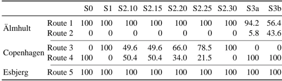
An important indicator of the impact of the studied transport measures is the route choice, which we illustrate with the percentage of TEUs transported using different routes. In Table 1 it can be seen that all of the studied measures caused a shift towards routes involving more rail transports and less road transports. However, for different measures the shift was observed in different parts of the network. For transportation to Älmhult, the only measure that showed an effect on the route choice is the South-East Link. In the settings without the SouthSouth-East Link, all TEUs were transported on road between Karlshamn and Älmhult (i.e., Route 1). In the settings with the South-East Link (S3a and S3b) we observed shifts toward Route 2 using the SouthSouth-East Link (i.e., railway). In S3a in average 5.8% and in S3b in average 43.6% of the TEUs were
transported using Route 2. Not surprisingly, in the setting with better timetable syn-chronization (S3b) we observed a higher shift than in the setting with slightly worse synchronization (S3a). In all settings, transportation of all TEUs to Esbjerg were made using Route 5, with sea transportation from Klaipeda to Fredericia followed by road transportation from Fredericia to Esbjerg. This is reasonable due to the fact that the long distance makes it economically tractable to use sea transportation instead of land transportation through Sweden and Denmark. For Copenhagen Customer, which can be reached only by truck, the results vary for the different settings. For settings S0 and S3, in which no measures were applied for transportation on the routes to Copenhagen Customer, all transports were made using road transportation from Karlshamn directly to Copenhagen Customer (i.e., Route 4). In setting S1 (kilometer tax), a 100 % shift towards Route 3 using rail between Karlshamn and Copenhagen Terminal followed by road transportation between Copenhagen Terminal and Copenhagen Customer was ob-served. For settings S2 (CO2 tax), a gradually increasing shift towards Route 3 was observed as the tax level was increased.
Table 1. For each setting and each customer, the average taken over 10 replications of the share
of TEUs (in percentage) transported using the different routes.
S0 S1 S2.10 S2.15 S2.20 S2.25 S2.30 S3a S3b Älmhult Route 1 100 100 100 100 100 100 100 94.2 56.4 Route 2 0 0 0 0 0 0 0 5.8 43.6 CopenhagenRoute 3 0 100 49.6 49.6 66.0 78.5 100 0 0 Route 4 100 0 50.4 50.4 34.0 21.5 0 100 100 Esbjerg Route 5 100 100 100 100 100 100 100 100 100
A positive consequence of achieving a shift from road to rail transportation is re-duced CO2emissions. All observed reductions of CO2emissions in the studied system is a consequence of a modal shift from road to rail in Sweden and Denmark. Therefore, in Fig. 3 we present the relative CO2reduction for (a) the whole system, and (b) land transports in Sweden and Denmark. The main reason for observing such a minor re-duction of CO2emissions when considering all simulated transports is that a significant share of the transports in all settings were made using sea and rail transportation be-tween Kaunas and Karlshamn and bebe-tween Klaipeda and Esbjerg. Further, the transport costs are affected in different ways by different measures and it may be important to analyze the positive effects (e.g., reduced CO2 emissions) in relation to the economic impact caused by applying measures. For the studied transport measures, we show in Table 2 the average costs for transporting one TEU to the different customers.
For transportation to Älmhult, we observed a very small change in transport cost when studying the effects of the SouthEast Link (S3a and S3b). The reason is that the costs for transportation by road and rail between Karlshamn and Älmhult in the studied scenario are rather similar. The cost for transportation to the customer in Copenhagen
Fig. 3. For each studied measure, the relative reduction (in percentage) of CO2emissions for (a) the whole system, and (b) land transports in Sweden and Denmark.
S1 S2.10 S2.15 S2.20 S2.25 S2.30 S3a S3b Relativ e reduction (%) 0.0 0.2 0.4 0.6 0.8 1.0
(a) Whole system
S1 S2.10 S2.15 S2.20 S2.25 S2.30 S3a S3b Relativ e reduction (%) 0 2 4 6 8 10 12
(b) Land transports in Sweden and Denmark
is affected both by the studied CO2tax and by the kilometer tax, since it is impossible to reach the customer without involving road transportation. The cost for transportation to Esbjerg is only influenced by an increased CO2tax, since all transports to Esbjerg is made with sea and rail transportation, which is not affected by the studied kilometer tax.
Table 2. For each setting, the average cost (in euro) for transporting one TEU to each customer.
S0 S1 S2.10 S2.15 S2.20 S2.25 S2.30 S3a S3b Älmhult 364.2 368.5 426.0 456.9 487.8 518.7 549.6 364.7 364.3 Copenhagen 554.8 566.3 627.3 660.9 695.4 729.4 764.5 554.9 554.8 Esbjerg 519.0 519.0 606.9 650.8 694.7 738.6 782.6 519.0 519.0
4
Discussion on how to conduct MABS studies for impact
assessment of transport measures
In this section, we discuss a number of aspects that are important to consider when using MABS for impact assessment of different types of transport measures. The dis-cussion is built around the TAPAS simulation tool described in Section 2 and the EWTC simulation study presented in Section 3, and we provide concrete examples of lessons learnt when working with TAPAS. Overviews of different aspects that are relevant to consider when conducting simulation studies can be found in the literature, e.g., design of simulation studies are discussed in [10, 9, 11], data collection in [16], verification and validation in [17], and output data analysis in [12].
The process of conducting a simulation study can be regarded as a process contain-ing three sequential phases; design, execution and analysis. In the design phase, the analyst finds out what should be done, and decides how it is appropriate to conduct the study. In the execution phase, input data is collected, scenarios are coded, and simula-tion runs are made. Finally, in the analysis phase, the output is analyzed and potentially generalized to enable general conclusions to be made. The process is typically iterative since there often is a need to return to previous phases and reconsider earlier decisions and activities. For example, from a pre-study it may be realized that the ambitions con-cerning data collection, generalization, complexity of the studied scenario, etc., may have to be revised.
4.1 General design decisions
Since the purpose of conducting a study will have a significant influence on other design decisions it is important to identify the purpose as early as possible in the process. Typical examples of purposes for conducting a simulation study include learning about what measures are required to reach a certain goal and gaining general knowledge about a particular system, e.g., by conducting a sensitivity analysis. In addition to establishing an underlying purpose for conducting the study, the identification of a purpose typically involves defining which measures are relevant to consider, as well as identifying what particular questions should be studied.
In the design phase of a MABS study for impact assessment of transport measures there are potentially many design questions that should be answered. Below we list a number of questions that are relevant to consider when designing a simulation study, of which some are general and also discussed in the literature [9]:
– What particular set of transport measures should be studied?
– What is the expected outcome of the study, i.e., which types of effects are expected? – What is an appropriate scope of the studied scenario considering complexity and
the potential to obtain useful results (e.g., concerning which physical entities and what geographical areas should be considered)?
– Should the scenario be calibrated towards current practice, and how should it be
calibrated?
– How should the scenario and the results be validated? – If (and how) should a sensitivity analysis be conducted?
– What output data is relevant to study, and how should the output be analyzed? – Is there a need to generalize the results, and how is it appropriate to obtain
gener-alizable results?
– From which data sources should data be collected, and how should data be
prepro-cessed?
– How should prices and costs be represented? Is it relevant to model estimated
in-ternal costs, or is it better to model market prices of services, which potentially include profit margins?
– Which physical entities should be represented, and how is it appropriate to model
them? For example, is it relevant to aggregate entities of the same type (e.g., product types as in the studied EWTC scenario)?
– How and which decision makers should be represented in the model, e.g.,
concern-ing how decision strategies are assigned to agents?
– How many simulation runs should be made, what parameter settings should be used
for the different runs, and how long should simulation runs be?
4.2 Input data management
When conducting a MABS study for impact assessment of transport measures, it is important to identify all entities that should be modeled, and describe them in an ap-propriate level of detail. Input data for describing physical entities, e.g., vehicle charac-teristics, link lengths and timetables, should be collected. In TAPAS, input distributions should be specified for consumption, production, and transportation. Also, strategies of modeled decision makers, specified as cost structures, need to be provided. In most re-alistic scenarios, this means that a large amount of input data need to be collected from various sources, and this is something that generally applies to micro-level simulation. There are several issues related to collecting input data, e.g., crucial (micro-level) data might be missing or difficult to obtain. Typical reasons are that data do not exist, or that organizations and enterprises that are holding information are unwilling to share detailed and accurate data. Further, the quality of available data may be low, and data collection may require too much time and effort. Therefore, the analyst sometimes needs to make a trade-off between how much effort should be spent on data collection and the possibility to obtain high quality data, and ultimately, high quality results.
If data is partially or completely inaccurate or missing, appropriate assumptions about the reality may have to be made to be able to represent those entities that are completely or partially unknown. For example, to be able to study certain transport related taxes and fees, it is sometimes necessary to break down the transport cost into cost parameters, such as time-based and distance-based costs. If the relations between these cost parameters are unknown, the analyst has to make proper assumptions and estimations. This is exactly what was done in the EWTC study, in which time-based and distance-based cost parameters were estimated and validated using interviews with domain experts and with macro-level data from the SAMGODS model [19].
Due to limited availability of data or when the need for a high level of detail in the scenario is low, it may sometimes be appropriate to aggregate multiple real-world entities into fewer entities in the model, e.g., by using available aggregated (macro-level) data. As an example, in the EWTC study producers have been aggregated and represented by a single logistical terminal, and product types are also represented on an aggregate level. On the contrary, if accurate data is available it is sometimes possible and relevant to represent a real world entity with multiple model entities, e.g., when the same type of entity is associated with different costs in different geographical areas. Moreover, depending on the purpose of a study, it is sometimes relevant to disregard input that is assumed to have little or no effect on the decision making and on the types of output that are studied. For example, if no measures or effects concerning emissions are considered, it is typically not relevant to provide input data related to emissions.
An option that is always possible when dealing with issues concerning availability of high-quality input data is to narrow the scope (e.g., geographical) of the scenario to a size for which appropriate data can be found. However, it is important to consider that
the validity and possibility for generalizing the results may be affected when assuming or aggregating data, or when the scope of the study is being reduced.
A question that is related to management of input data is if internal cost structures of the modeled companies should be modeled, or if it is better to model market prices of services, potentially including profit margins. It should be noted that it often is difficult to obtain data that accurately estimate internal cost structures, e.g., since companies are unwilling to share data, or since the study concerns future scenarios for which no real-world data exists. It might be better to use market prices when they appear to be rather stable and representative for long-term prices of transport services whereas internal costs, if available, might be more suitable in other cases. Internal costs may have the advantage to better represent different cost components (e.g., time- and distance-based costs), which might be important when analyzing different transport measures, whereas market prices rarely are given explicitly for different cost components. Also, internal cost estimates might be more accurate in case of non-stable or unknown market prices, e.g., if a new market or newly introduced product types are studied.
4.3 Validation, verification and calibration
Validation, verification, and calibration of simulation models and scenarios are impor-tant in order to obtain valid and credible results [13]. Verification concerns whether an implemented simulation model represents a correct mapping of the conceptual model. Validation is about determining if the conceptual model represents a correct mapping of the modeled system. Calibration is about tuning the parameters of a simulation model or a scenario, typically in an iterative manner by comparing simulation output to real system output, in order to obtain valid simulation results. Complete validity is often difficult to obtain, and the level of validity and credibility that is needed depends on the purpose of the model [17]. A considerable amount of effort typically has to be put into setup and calibration of scenarios. It should be noted that the process of conducting simulation experiments typically contributes to the validity of the model.
From the wide range of available techniques for validation and verification (see [17] for an overview), it is the responsibility of the analyst to determine on case basis how the validity should be shown. A few examples of techniques that can be used include:
– Involving decision makers and policy makers when developing scenarios.
– Comparing results with historic and recent real-world data, with statistics
concern-ing activities in the studied area, and with results obtained with other models.
– Conducting sensitivity analyses of certain input parameters and assess the behavior
of the studied system.
– Performing pre-studies with small versions of the scenario, which would make the
results easier to compare with analytically generated output and enabling results to be compared with what is to be logically expected.
Moreover, to (partially) validate a model or a scenario, it is possible to use concep-tual validation, i.e., “determining that the theories and assumptions underlying the con-ceptual model are correct and that the model representation of the problem entity is ’reasonable’ for the intended purpose of the model” [17].
We believe it is important to involve different stakeholders in the process of formu-lating scenarios. By making use of participatory modeling, the process of formuformu-lating a scenario will also be part of the process of understanding and analyzing the impact of transport measures. The EWTC scenario was developed in collaboration with a number of relevant stakeholders, such as, transport authorities, transport operators and regional government, from three countries. A rough sketch of the scenario, including the scope of the scenario, interesting transport measures, relevant effects and types of goods, etc., was developed during discussions in this group. Then the simulation experts developed a more detailed scenario, which was presented to the group. After a discussion the group proposed some refinements of the suggested scenario. When the simulation experiments had been run, the results were analyzed within the group.
Involving policy makers and transport companies in the design of a MABS model is also important to discuss which aspects are necessary, relevant and desirable to repre-sent. In the case of TAPAS, the model was developed in projects with the involvement of various transport companies, transport analysts, and policy makers, and this process is still ongoing in a couple of projects even if the model already is implemented.
A typical approach when conducting a simulation study is to compare the results of a base scenario, which often is calibrated to correspond to the current situation, with the results of a number of situations in which one or more measures are applied. Parame-ters should (if possible) be calibrated in a way that the base scenario and the extended scenarios are affected in a similar way, however, this is something that can be difficult to achieve.
In real-world transport chains, decisions that are ineffective from a cost perspective are sometimes taken, e.g., due to old habit or since costs are estimated incorrectly by decision makers. If a purpose is to mimic a current (potentially non-optimal) situation, it is possible to compensate for non-optimal behavior by calibrating certain input pa-rameters (costs, load utilization factors, etc.). A further possibility is to explicitly model non-optimal behavior of real-world decision makers, e.g., by modeling that it may take some time before a change of transport solution occurs, even though there exists other more beneficial solutions. It would also be possible to let factors such as environmental impact, reliability and punctuality, explicitly influence the decision making. Another reason for calibrating a scenario (other than representing non-optimal behavior) is to compensate for errors in input data.
4.4 Result analysis and generalization
In TAPAS, all input data and activities that occur during a simulation run are logged in a database, which makes it possible to reproduce and carefully analyze simulation runs afterwards. We argue that it could be a good idea to keep a database containing all relevant information concerning a simulation run, in contrast to just saving specific types of output, unless this is considered infeasible from a performance perspective. This is due to the fact that it could be realized late in a study what particular output data is needed. However, for large scenarios that create huge amount of output data, it is often impractical, or even impossible, to store all data that is produced during a simulation run. Examples of relevant output data that can be extracted from TAPAS are choices of vehicle types and transport routes, order sizes and frequencies, transport
times, transport costs, environmental performance (e.g., CO2emissions), and transport work (ton kilometers).
The output from TAPAS can be categorized into economical, logistical, and envi-ronmental, which makes it possible to use TAPAS for multi-criteria analysis. In the EWTC scenario, CO2emissions, costs, and modal split were analyzed, enabling the an-alyst and policy makers to use multiple aspects when analyzing the results of a transport measure, or when assessing if the expected impact of a transport measure is sufficiently sustainable. An advantage of making use of MABS for transport policy analysis is that the results become rather concrete and straight-forward to relate to actual effects.
Since simulation often is considered to be a statistical experiment (activities occur according to stochastic input distributions), the output will also be randomly distributed. In TAPAS, consumption, transportation and production is described using random dis-tributions, and to be able to draw strong conclusions, it is important to manage statistics in a proper way, e.g., by choosing input distributions carefully and analyzing output sta-tistically. Output data can be analyzed using significance tests, correlation analyses, and by generating confidence intervals (e.g., [12]). Also, to obtain statistical significance, a larger number of replications typically need to be run for each studied setting.
Depending on what types of questions are studied, there is sometimes a wish to gen-eralize the results. Due to difficulties regarding performance of micro-level simulation and collection of real-world data, it may be appropriate to study limited transport net-works when using MABS models. However, generalizable results can still be obtained by studying a larger number of smaller scenarios in which, e.g., the location and char-acteristics of customers and producers are randomly varied. By simulating a range of different actors and settings, it is typically possible to observe more general tendencies than can be obtained by only simulating smaller networks.
5
Concluding remarks
We have provided a discussion on how it is appropriate to design and conduct simula-tion studies when using MABS for impact assessment of transport policy and infras-tructure measures (transport measures). The discussion concerns general design issues, input data management, validation and verification, calibration, output data analysis, and generalization of results. Specific aspects that are covered in the discussion are par-ticipatory and collaborative modeling and simulation, selection of which entities and aspects to include in a simulation study, and how multi-criteria analysis can be used with MABS when analyzing transport measures. Further, the discussion is built around the TAPAS simulation tool (see Section 2) and an EWTC simulation study (see Sec-tion 3), which illustrates how it is possible to analyze transport measures by studying modal split, CO2emissions, and transport costs.
We conclude the paper by stating that we believe that our work may be a valuable resource when (1) developing new MABS models for impact assessment of transport measures, since it is important already at the development phase to account for how to use the model, and (2) conducting simulation studies using existing models, since our discussion covers most aspects that are relevant to consider when conducting a study for impact assessment of transport measures.
Acknowledgements
We wish to thank our colleagues in the EWTC I and II projects for valuable feedback. The research is part-financed by the European Union (European Regional Development Fund and European Neighbourhood and Partnership Instrument, Baltic Sea Region Pro-gramme 2007-2013) via the EWTC II project.
References
1. Button, K.: Transport Economics. Edward Elgar Publishing Limited, Glos, UK, 2nd edn. (1997)
2. Davidsson, P., Holmgren, J., Persson, J.A., Ramstedt, L.: Multi agent based simulation of transport chains. In: Proceedings of the 7th international joint conference on Autonomous agents and multiagent systems (AAMAS 2008). pp. 1153–1160. International Foundation for Autonomous Agents and Multiagent Systems, May 12-16, Estoril, Portugal (2008) 3. de Jong, G., Ben-Akiva, M.: A micro-simulation model of shipment size and transport chain
choice. Transportation Research Part B 41(9), 950–965 (2007)
4. European Commission: White paper - European transport policy for 2010: time to decide. Tech. rep., Luxemburg (2001)
5. Friberg, G., Flack, M., Hill, P., Johansson, M., Vierth, I., McDaniel, J., Lundgren, T., Hes-selborn, P., Bångman, G.: Kilometerskatt för lastbilar - Effekter på näringar och regioner. Redovisning av ett regeringsuppdrag i samverkan med ITPS, Report 2007:2, Swedish Insti-tute for Transport and Communications Analysis (SIKA) (2007)
6. Gambardella, L., Rizzoli, A., Funk, P.: Agent-based planning and simulation of combined rail/road transport. Simulation 78(5), 293–303 (2002)
7. Holmgren, J.: An extended EastWest Transport Corridor (EWTC) scenario (2011), Available at: http://www.bth.se/tek/jhm.nsf/attachments/eewtc_pdf/$file/eewtc.pdf
8. Holmgren, J., Davidsson, P., Persson, J.A., Ramstedt, L.: TAPAS: A multi-agent-based model for simulation of transport chains. Simulation Modelling Practice and Theory 23, 1–18 (2012)
9. Kelton, W.D., Barton, R.R.: Experimental design for simulation. In: Proceedings of the 2003 Winter Simulation Conference. pp. 59–65. IEEE, December 7-10, New Orleans, Louisiana, USA (2003)
10. Kleijnen, J.P.C.: An overview of the design and analysis of simulation experiments for sen-sitivity analysis. European Journal of Operational Research 164(2), 287–300 (2005) 11. Kleijnen, J.P.C.: Design of experiments: overview. In: Proceedings of the 2008 Winter
Sim-ulation Conference. pp. 479–488. IEEE, December 7-10, Miami, Florida, USA (2008) 12. Law, A.M.: Statistical analysis of simulation output data: the practical state of the art. In:
Proceedings of the 2007 Winter Simulation Conference. pp. 77–83. IEEE, December 9-12, Washington, DC, USA (2007)
13. Law, A.M., Kelton, W.D.: Simulation modelling and analysis. McGraw-Hill, Singapore, 3rd edn. (2000)
14. Liedtke, G.: Principles of micro-behavior commodity transport modeling. Transportation Re-search Part E 45(5), 795–809 (2009)
15. Rich, J., Bröcker, J., Hansen, C.O., Korchenewych, A., Nielsen, O.A., Vuk, G.: Report on scenario, traffic forecast and analysis of traffic on the TEN-T, taking into consideration the external dimension of the union - TRANS-TOOLS version 2; Model and data improvements. Tech. rep., Copenhagen, Denmark (2009)
16. Sapsford, R., Jupp, V. (eds.): Data collection and analysis. SAGE Publications Ltd, Chennai, India, 2nd edn. (2006)
17. Sargent, R.G.: Verification and validation of simulation models. In: Proceedings of the 2005 Winter Simulation Conference. pp. 130–143. IEEE, December 4-7, Orlando, Florida, USA (2005)
18. SIKA: Vilken koldioxidskatt krävs för att nå framtida utsläppsmål? PM 2008:4, Swedish Institute for Transport and Communications Analysis (SIKA) (2008)
19. Swahn, H.: The Swedish national model systems for goods transport SAMGODS - a brief introductory overview. SAMPLAN Report 2001:1, Swedish Institute for Transport and Com-munications Analysis (SIKA) (2001)
20. Tavasszy, L., Smeenk, B., Ruijgrok, C.: A DSS for modelling logistic chains in freight transport policy analysis. International Transactions in Operational Research 5(6), 447–459 (1998)