https://doi.org/10.1051/0004-6361/201833764 c ESO 2018
Astronomy
&
Astrophysics
Extended transition rates and lifetimes in Al i and Al ii from
systematic multiconfiguration calculations
?
A. Papoulia (
AshmÐna PapoÔlia)
1,2, J. Ekman
1, and P. Jönsson
1 1 Materials Science and Applied Mathematics, Malmö University, 20506 Malmö, Swedene-mail: asimina.papoulia@mau.se
2 Division of Mathematical Physics, Lund University, Post Office Box 118, 22100 Lund, Sweden
Received 3 July 2018/ Accepted 22 September 2018
ABSTRACT
MultiConfiguration Dirac-Hartree-Fock (MCDHF) and relativistic configuration interaction (RCI) calculations were performed for 28 and 78 states in neutral and singly ionized aluminium, respectively. In Al i, the configurations of interest are 3s2nl for n= 3, 4, 5 with
l= 0 to 4, as well as 3s3p2and 3s26l for l= 0, 1, 2. In Al ii, in addition to the ground configuration 3s2, the studied configurations
are 3snl with n = 3 to 6 and l = 0 to 5, 3p2, 3s7s, 3s7p, and 3p3d. Valence and core-valence electron correlation effects are
systematically accounted for through large configuration state function (CSF) expansions. Calculated excitation energies are found to be in excellent agreement with experimental data from the National Institute of Standards and Technology (NIST) database. Lifetimes and transition data for radiative electric dipole (E1) transitions are given and compared with results from previous calculations and available measurements for both Al i and Al ii. The computed lifetimes of Al i are in very good agreement with the measured lifetimes in high-precision laser spectroscopy experiments. The present calculations provide a substantial amount of updated atomic data, including transition data in the infrared region. This is particularly important since the new generation of telescopes are designed for this region. There is a significant improvement in accuracy, in particular for the more complex system of neutral Al i. The complete tables of transition data are available at the CDS.
Key words. atomic data
1. Introduction
Aluminium is an important element in astrophysics. In newly born stars the galactic [Al/H] abundance ratio and the [Al/Mg] ratio are found to be increased in comparison to early stars (Clayton 2003). The aluminium abundance and its anti-correlation with that of magnesium is the best tool to determine which generation a globular cluster star belongs to. The abun-dance variations of different elements and the relative numbers of first- and second-generation stars can be used to determine the nature of polluting stars, the timescale of the star forma-tion episodes, and the initial mass funcforma-tion of the stellar cluster (Carretta et al. 2010). The aluminium abundance is of impor-tance for other types and groups of stars as well. A large num-ber of spectral lines of neutral and singly ionized aluminium are observed in the solar spectrum and in many stellar spectra. Aluminium is one of the interesting elements for chemical anal-ysis of the Milky Way, and one example is the Gaia-ESO Sur-vey1; medium- and high-resolution spectra from more than 105
stars are analysed to provide public catalogues with astrophys-ical parameters. As part of this survey, Smiljanic et al. (2014) analysed high-resolution UVES2 spectra of FGK-type stars and derived abundances for 24 elements, including aluminium.
? The data are only available available at the CDS via anonymous ftp
tocdsarc.u-strasbg.fr(130.79.128.5) or viahttp://cdsarc.
u-strasbg.fr/viz-bin/qcat?J/A+A/621/A16
1 http://casu.ast.cam.ac.uk/surveys-projects/ges
2 http://www.eso.org/sci/facilities/paranal/
instruments/uves.html
In addition, aluminium abundances have been determined in local disk and halo stars by Gehren et al.(2004), Reddy et al. (2006), Mishenina et al. (2008), Adibekyan et al. (2012), and Bensby et al.(2014). However, chemical evolution models still have problems reproducing the observed behaviour of the alu-minium abundance in relation to abundances of other ele-ments. Such examples are the observed trends of the aluminium abundances in relation to metallicity [Fe/H], which are not well reproduced at the surfaces of stars, for example giants and dwarfs (Smiljanic et al. 2016). In light of the above issues, Smiljanic et al. (2016) redetermined aluminium abundances within the Gaia-ESO Survey. Furthermore, strong deviations from local thermodynamic equilibrium (LTE) are found to sig-nificantly affect the inferred aluminium abundances in metal poor stars, which was highlighted in the work byGehren et al. (2006).Nordlander & Lind (2017) presented a non-local ther-modynamic equilibrium (NLTE) modelling of aluminium and provided abundance corrections for lines in the optical and near-infrared regions.
Correct deduction of aluminium abundances and chemical evolution modelling is thus necessary to put together a complete picture of the stellar and Galactic evolution. Obtaining the spec-troscopic reference data to achieve this goal is demanding. A significant amount of experimental research has been conducted to probe the spectra of Al ii and Al i and to facilitate the analy-sis of the astrophysical observations. Even so, some laboratory measurements still lack reliability and in many cases, especially when going to higher excitation energies, only theoretical values of transition properties exist. Accurate computed atomic data are
therefore essential to make abundance analyses in the Sun and other stars possible.
For the singly ionized Al ii, there are a number of mea-surements of transition properties. The radiative lifetime of the 3s3p3Po
1 level was measured by Johnson et al. (1986) using
an ion storage technique and the transition rate value for the inter-combination 3s3p3Po
1 → 3s
2 1S
0transition was provided.
Träbert et al. (1999) measured lifetimes in an ion storage ring and the result for the lifetime of the 3s3p3Po
1 level is in
excel-lent agreement with the value measured byJohnson et al.(1986). Using the beam-foil technique, Andersen et al. (1971) mea-sured lifetimes for the 3snf3F series with n = 4−7, although
these measurements are associated with significant uncertain-ties. By using the same technique, the lifetime of the sin-glet 3s3p1Po1 level was measured in four different experimental works (Kernahan et al. 1979;Head et al. 1976;Berry et al. 1970; Smith 1970), which are in very good agreement.
In the case of neutral Al i, several measurements have also been performed. Following a sequence of earlier works (Jönsson & Lundberg 1983;Jönsson et al. 1984),Buurman et al. (1986) used laser spectroscopy to obtain experimental values for the oscillator strengths of the lowest part of the spec-trum. A few years later,Buurman & Dönszelmann(1990) rede-termined the lifetime of the 3s24p2P level and separated the different fine-structure components. Using similar laser tech-niques,Davidson et al.(1990) measured the natural lifetimes of the 3s2nd2D Rydberg series and obtained oscillator strengths
for transitions to the ground state. In a more recent work, Vujnovi´c et al.(2002) used the hollow cathode discharge method to measure relative intensities of spectral lines of both neutral and singly ionized aluminium. Absolute transition probabilities were evaluated based on available results from previous studies, such as the ones mentioned above.
Al ii is a nominal two-electron system and the lower part of its spectrum is strongly influenced by the interaction between the 3s3d1D and 3p2 1D configuration states. Contrary to
neu-tral Mg i where no level is classified as 3p2 1D, in Al ii the
3p2 configuration dominates the lowest 1D term and yields a well-localized state below the 3s3d1D term. The interactions
between the 3snd1D Rydberg series and the 3p2 1D perturber were investigated byTayal & Hibbert(1984). Going slightly fur-ther up, the spectrum of Al ii is governed by the strong mixing of the 3snf3F Rydberg series with the 3p3d3F term. Despite
the widespread mixing, 3p3d3F is also localized, between
the 3s6f3F and 3s7f3F states. The configuration interaction
between doubly excited states (e.g. the 3p2 1D and 3p3d3F
states) and singly excited 3snl1,3L states was thoroughly inves-tigated by Chang & Wang(1987). However, the extreme mix-ing of the 3p3d3F term in the 3snf3F series and its effect on the computation of transition properties was first investigated byWeiss(1974). Although the work byChang & Wang(1987) was more of a qualitative nature, computed transition data were provided based on configuration interaction (CI) calculations. Using the B-spline configuration interaction (BSCI) method, Chang & Fang (1995) also predicted transition properties and lifetimes of Al ii excited states.
Despite the large number of measured spectral lines in Al i, the 3s3p2 2D state could not be experimentally identified and for a long time theoretical calculations had been trying to localize it and predict whether it lies above or below the first-ionization limit. Al i is a system with three valence electrons, and the correlation effects are even stronger than in the singly ionized Al ii. Especially strong is the two-electron interaction of 3s3d1D with 3p2 1D, which becomes evident between the 3s23d2D and
3s3p2 2D states. The 3s3p2 2D state is strongly coupled to the 3s23d2D state, but it is also smeared out over the entire discrete
part of the 3s2nd2D series and contributes to a significant mix-ing of all those states (Weiss 1974). Asking for the position of the 3s3p2 2D level is thus meaningless since it does not
corre-spond to any single spectral line (Lin 1974;Trefftz 1988). Due to this strong two-electron interaction, the line strength of one of the2D states involved in a transition appears to be enhanced, while the line strength of the other2D state is suppressed. This
makes the computation of transition properties in Al i far from trivial (Froese Fischer et al. 2006). More theoretical studies on the system of neutral aluminium were conducted byTaylor et al. (1988) andTheodosiou(1992).
In view of the great astrophysical interest for accurate atomic data, close coupling (CC) calculations were carried out for the systems of Al ii and Al i by Butler et al. (1993) and Mendoza et al. (1995), respectively, as part of the Opac-ity Project. These extended spectrum calculations produced transition data in the infrared region (IR), which had been scarce until then. However, the neglected relativistic effects and the insufficient amount of correlation included in the calcula-tions constitute limiting factors to the accuracy of the results. Later on, Froese Fischer et al. (2006) performed MultiConfig-uration Hartree-Fock (MCHF) calculations and used the Breit-Pauli (BP) approximation to also capture relativistic effects for Mg- and Al-like sequences. Focusing more on correlation, rel-ativistic effects were kept to lower order. Even so, in Al i, correlation in the core and core-valence effects were not included due to limited computational resources. The latest compila-tion of Al ii and Al i transicompila-tion probabilities was made available byKelleher & Podobedova(2008a).Wiese & Martin(1980) had earlier updated the first critical compilation of atomic data by Wiese et al.(1969).
Although for the past decades a considerable amount of research has been conducted for the systems of Al ii and Al i, there is still a need for extended and accurate theoretical tran-sition data. The present study is motivated by such a need. To obtain energy separations and transition data, the fully relativis-tic MultiConfiguration Dirac-Hartree-Fock (MCDHF) scheme has been employed. Valence and core-valence electron correla-tion is included in the computacorrela-tions of both systems. Spectrum calculations have been performed to include the first 28 and 78 lowest states in neutral and singly ionized aluminium, respec-tively. Transition data corresponding to IR lines have also been produced. The excellent description of energy separations is an indication of highly accurate computed atomic properties, which can be used to improve the interpretation of abundances in stars.
2. Theory
2.1. MultiConfiguration Dirac-Hartree-Fock approach
The wave functions describing the states of the atom, referred to as atomic state functions (ASFs), are obtained by applying the MCDHF approach (Grant 2007;Froese Fischer et al. 2016). In the MCDHF method, the ASFs are approximate eigenfunctions of the Dirac-Coulomb Hamiltonian given by
HDC = N X i=1 [c αi· pi+ (βi− 1)c2+ Vnuc(ri)]+ N X i< j 1 ri j , (1)
where Vnuc(ri) is the potential from an extended nuclear charge
distribution, α and β are the 4 × 4 Dirac matrices, c the speed of light in atomic units, and p ≡ −i∇ the electron momentum
operator. An ASFΨ(γPJMJ) is given as an expansion over NCSF
configuration state functions (CSFs),Φ(γiPJ MJ), characterized
by total angular momentum J and parity P:
Ψ(γPJMJ)= NCSF
X
i=1
ciΦ(γiPJ MJ). (2)
The CSFs are anti-symmetrized many-electron functions built from products of one-electron Dirac orbitals and are eigen-functions of the parity operator P, the total angular momen-tum operator J2and its projection on the z-axis Jz(Grant 2007;
Froese Fischer et al. 2016). In the expression above, γi
repre-sents the configuration, coupling, and other quantum numbers necessary to uniquely describe the CSFs.
The radial parts of the Dirac orbitals together with the mixing coefficients ciare obtained in a self-consistent field (SCF)
pro-cedure. The set of SCF equations to be iteratively solved results from applying the variational principle on a weighted energy functional of all the studied states according to the extended opti-mal level (EOL) scheme (Dyall et al. 1989). The angular inte-grations needed for the construction of the energy functional are based on the second quantization method in the coupled tensorial form (Gaigalas et al. 1997,2001).
The transverse photon (Breit) interaction and the leading quantum electrodynamic (QED) corrections (vacuum polar-ization and self-energy) can be accounted for in subse-quent relativistic configuration interaction (RCI) calculations (McKenzie et al. 1980). In the RCI calculations, the Dirac orbitals from the previous step are fixed and only the mixing coefficients of the CSFs are determined by diagonalizing the Hamiltonian matrix. All calculations were performed using the relativistic atomic structure package GRASP2K (Jönsson et al. 2013).
In the MCDHF relativistic calculations, the wave functions are expansions over j j-coupled CSFs. To identify the computed states and adapt the labelling conventions followed by the exper-imentalists, the ASFs are transformed from j j-coupling to a basis of LS J-coupled CSFs. In the GRASP2K code this is done using the methods developed by Gaigalas et al. (2003, 2004, 2017).
2.2. Transition parameters
In addition to excitation energies, lifetimes τ and transition parameters, such as emission transition rates A and weighted oscillator strengths g f , were also computed. The transition parameters between two states γ0P0J0and γPJ are expressed in terms of reduced matrix elements of the transition operator T (Grant 1974):
hΨ(γPJ)||T||Ψ(γ0P0J0)i=X
k,l
ckc0lhΦ(γkPJ)||T||Φ(γ0lP0J0)i. (3)
For electric multipole transitions, there are two forms of the transition operator: the length, which in fully relativistic calcu-lations is equivalent to the Babushkin gauge, and the velocity form, which is equivalent to the Coulomb gauge. The transi-tions are governed by the outer part of the wave functransi-tions. The length form is more sensitive to this part of the wave func-tions and it is generally considered to be the preferred form. Regardless, the agreement between the values of these two dif-ferent forms can be used to indicate the accuracy of the wave functions (Froese Fischer 2009;Ekman et al. 2014). This is par-ticularly useful when no experimental measurements are avail-able. The transitions can be organized in groups determined, for
instance, by the magnitude of the transition rate value. A statis-tical analysis of the uncertainties of the transitions can then be performed. For each group of transitions the average uncertainty of the length form of the computed transition rates is given by
hdT i= 1 N N X i=1 |Ai l− A i υ| max(Ai l, A i υ) , (4)
where Al and Aυ are respectively the transition rates in length
and velocity form for a transition i and N is the number of the transitions belonging to a group. In this work, we only computed transition parameters for the electric dipole (E1) transitions. The electric quadrupole (E2) and magnetic multipole (Mk) transi-tions are much weaker and therefore less likely to be observed.
3. Calculations
3.1. Al I
In neutral aluminium, calculations were performed in the EOL scheme (Dyall et al. 1989) for 28 targeted states. These states belong to the 3s2ns configurations with n = 4, 5, 6, the 3s2nd configurations with n = 3, ..., 6, and the 3s3p2 and 3s25g
con-figurations, characterized by even parity, and on the other hand the 3s2np configurations with n= 3, .., 6 and the 3s24f and 3s25f
configurations, characterized by odd parity. These configurations define what is known as the multireference (MR). From initial calculations and analysis of the eigenvector compositions, we deduced that all 3p2nl configurations, in addition to the targeted
3s2nl, give considerable contributions to the total wave
func-tions and should be included in the MR. Following the active set (AS) approach (Olsen et al. 1988;Sturesson et al. 2007), the CSF expansions (see Eq. (2)) were obtained by allowing single and restricted double (SD) substitutions of electrons from the reference (MR) orbitals to an AS of correlation orbitals. The AS is systematically increased by adding layers of orbitals to e ffec-tively build nearly complete wave functions. This is achieved by keeping track of the convergence of the computed excitation energies, and of the other physical quantities of interest, such as the transition parameters here.
As a first step an MCDHF calculation was performed for the orbitals that are part of the MR. States with both even and odd parity were simultaneously optimized. Following this step, we continued to optimize six layers of correlation orbitals based on valence (VV) substitutions. The VV expansions were obtained by allowing SD substitutions from the three outer valence orbitals in the MR, with the restriction that there will be at most one substitution from orbitals with n = 3. In this manner, the correlation orbitals will occupy the space between the inner n= 3 valence orbitals and the outer orbitals involved in the higher Rydberg states (see Fig. 1). These orbitals have been shown to be of crucial importance for the transition prob-abilities, which are weighted towards this part of the space (Pehlivan Rhodin et al. 2017; Pehlivan Rhodin 2018). The six correlation layers correspond to the 12s, 12p, 12d, 11f, 11g, and 10h set of orbitals.
Each MCDHF calculation was followed by an RCI calcu-lation for an extended expansion, obtained by single, double, and triple (SDT) substitutions from the valence orbitals. As a final step, an RCI calculation was performed for the largest SDT valence expansion augmented by a core-valence (CV) expansion. The CV expansion was obtained by allowing SD substitutions from the valence orbitals and the 2p6 core, with the restriction that there will be at most one substitution from
A&A proofs: 0 2 4 6 8 10 12
sqrt(r)
-0.5 0 0.5 1 1.5P(r)
2p 3p 4p 5p 6pFig. 1.Al i Dirac-Fock radial orbitals for the p symmetry, as a function
of √r. The 2p orbital is part of the core and the orbitals from n = 3 to n = 6 are part of the valence electron cloud. These orbitals occupy different regions in space and the overlap between some of the Rydberg states is minor.
2p6. All the RCI calculations included the Breit interaction and
the leading QED effects. Accounting for CV correlation does not lower the total energies significantly, but it can have large effects on the energy separations and thus we considered it cru-cial. Core-valence correlation is also important for transition properties (Hibbert 1989). Core-core (CC) correlation, obtained by allowing double excitations from the core, is known to be less important and has not been considered in the present work. The number of CSFs in the final even and odd state expan-sions, accounting for both VV and CV electron correlation, were 4 362 628 and 2 889 385, respectively, distributed over the di ffer-ent J symmetries.
3.2. Al II
In the singly ionized aluminium, the calculations were more extended, including 78 targeted states. These states belong to the 3s2 ground configuration, and to the 3p2; the 3sns
config-urations with n = 4, ..., 7; the 3snd with n = 3, ..., 6; and the 3s5g and 3s6g configurations, characterized by even parity, and on the other hand, the 3snp configurations with n = 3, ..., 7; the 3snf with n = 4, 5, 6; and the 3s6h and 3p3d configurations, characterized by odd parity. These configurations define the mul-tireference (MR). In the computations of Al ii, the EOL scheme was applied and the CSF expansions were obtained following the active set (AS) approach, accounting for VV and CV corre-lation. Al ii is less complex and the CSF expansions generated from (SD) substitutions are not as large as those in Al i. Hence, we can afford both 2s and 2p orbitals to account for CV cor-relation. The 1s core orbital remained closed and, as it was for Al i, core-core correlation was neglected. The MCDHF calcula-tions were performed in a similar way to the calculacalcula-tions in Al i, yet no particular restrictions were imposed on the VV substitu-tions. We optimized six correlation layers corresponding to the 13s, 13p, 12d, 12f, 12g, 8h, and 7i set of orbitals. Each MCDHF calculation was followed by an RCI calculation. Finally, an RCI calculation was performed for the largest SD valence expansion augmented by the CV expansion. The number of CSFs in the final even and odd state expansions, accounting for both VV and CV electron correlation, were 911 795 and 1 269 797, respec-tively, distributed over the different J symmetries.
4. Results
4.1. Al I
In Table1the computed excitation energies, based on VV cor-relation, are given as a function of the increasing active set of orbitals. After adding the n = 11 correlation layer, we note that the energy values for all 28 targeted states have converged. For comparison, in the second last column the observed ener-gies from the National Institute of Standards and Technology (NIST) Atomic Spectra Database (Kramida et al. 2018) are dis-played. All energies but those belonging to the 3s3p2 configura-tion are already in good agreement with the NIST recommended values. The relative differences between theory and experiment for all three levels of the quartet 3s3p2 4P state is 3.1%, while
the mean relative difference for the rest of the states is less than 0.2%. In the third last column, the computed excitation energies after accounting for CV correlation are displayed. When taking into account CV effects the agreement with the observed val-ues is better overall. Most importantly, for the 3s3p2 4P levels
the relative differences between observed and computed values decrease to less than 0.6%. The likelihood that the 1s22s22p6
core overlaps with the 3s3p2cloud of electrons is much less than that for 3s2nl. Consequently, when CV correlation is taken into
account the lowering of the 3s3p2energy levels is much smaller
than for levels belonging to any 3s2nl configuration. Thus, the
adjustments to the separation energies will be minor between the ground state 3s23p and 3s2nl levels, but significant between the 3s23p and 3s3p2levels. In the last column of Table1the
dif-ferences∆E = Eobs− Etheor, between the final (CV) computed
and the observed energies, are also displayed. In principle, there are two groups of values; the one consisting of the 3s2nd con-figurations exhibits the smallest absolute discrepancies from the observed energies. For the rest, the absolute discrepancies are somewhat larger.
In the calculations, the labelling of the eigenstates is deter-mined by the CSF with the largest coefficient in the expansion of Eq. (2). When the same label is assigned to different eigen-states, a detailed analysis can be performed by displaying their LS-compositions. In Table1, we note that two of the states have been assigned the same label, i.e. 3s24d2D, and thus the
sub-scripts a and b are used to distinguish them. In Table2, we give the LS -composition of all computed 3s2nd2D states,
includ-ing the three most dominant CSFs. The 3s24d2D term appears twice as the CSF with the largest LS -composition. Moreover, the admixture of the 3s3p2 2D in the four lowest 3s2nd2D states is rather strong and adds up to 65%. That being so, the 3s3p2 2D
does not exist in the calculated spectrum as a localized state. For comparison, in the last column of Table2 the labelling of the observed 3s2nd2D states is also given. In the observed
con-figurations presented by NIST (Kramida et al. 2018), the second highest 3s2nd2D term has not been given any specific label and
it is therefore designated as y2D. The higher2D terms are des-ignated as 3s24d, 3s25d, and so on.
In Table3, the current results for the lowest excitation ener-gies are compared with the values from the MCHF-BP calcu-lations by Froese Fischer et al. (2006). The latter calculations are extended up to levels corresponding to the doublet 3s24p2P
state. The differences ∆E between observed and computed ener-gies are given in the last two columns for the different com-putational approaches. As can be seen, when using the current MCDHF and RCI method the agreement with the observed ener-gies is substantially improved for all levels and in particular, for those belonging to the quartet 3s3p2 4P state. In the MCHF-BP calculations, core-valence correlation was neglected. As
Table 1. Computed excitation energies in cm−1
for the 28 lowest states in Al i.
VV
Pos. Conf. LS J n= 7 n= 8 n= 9 n= 10 n = 11 n = 12 CV Eobsa ∆E
1 3s23p 2Po1/2 0 0 0 0 0 0 0 0 0 2 2Po 3/2 108 108 108 108 108 108 104 112 8 3 3s24s 2S 1/2 25 318 25 377 25 416 25 419 25 427 25 429 25 196 25 348 152 4 3s 3p2 4P1/2 27 788 27 966 28 073 28 085 28 109 28 111 28 863 29 020 157 5 4P3/2 27 833 28 011 28 118 28 130 28 154 28 156 28 907 29 067 160 6 4P 5/2 27 906 28 085 28 191 28 204 28 227 28 230 28 981 29 143 162 7 3s23d 2D3/2 32 211 32 077 32 135 32 139 32 150 32 150 32 414 32 435 21 8 2D 5/2 32 212 32 079 32 137 32 141 32 152 32 152 32 416 32 437 21 9 3s24p 2Po 1/2 32 770 32 879 32 935 32 937 32 946 32 949 32 801 32 950 149 10 2Po 3/2 32 786 32 894 32 951 32 952 32 962 32 964 32 814 32 966 152 11 3s25s 2S1/2 37 493 37 637 37 693 37 694 37 704 37 706 37 512 37 689 177 12 3s24d 2D 3/2 a 38 733 38 659 38 711 38 707 38 717 38 718 38 951 38 929 −22 13 2D 5/2 a 38 736 38 664 38 717 38 712 38 722 38 724 38 957 38 934 −23 14 3s25p 2Po1/2 40 038 40 187 40 252 40 249 40 259 40 262 40 101 40 272 171 15 2Po 3/2 40 043 40 193 40 258 40 255 40 265 40 268 40 106 40 278 172 16 3s24f 2Fo 5/2 41 050 41 209 41 282 41 287 41 297 41 300 41 163 41 319 156 17 2Fo 7/2 41 050 41 209 41 282 41 287 41 297 41 300 41 163 41 319 156 18 3s26s 2S1/2 41 897 42 069 42 133 42 135 42 144 42 143 41 964 42 144 180 19 3s24d 2D 3/2 b 42 105 42 071 42 121 42 108 42 119 42 121 42 232 42 234 2 20 2D 5/2 b 42 109 42 075 42 126 42 112 42 123 42 125 42 237 42 238 1 21 3s26p 2Po1/2 43 076 43 246 43 316 43 311 43 321 43 324 43 160 43 335 175 22 2Po 3/2 43 079 43 249 43 318 43 313 43 324 43 326 43 162 43 338 176 23 3s25f 2Fo 5/2 43 549 43 721 43 795 43 801 43 811 43 813 43 660 43 831 171 24 2Fo 7/2 43 549 43 721 43 795 43 801 43 811 43 813 43 660 43 831 171 25 3s25g 2G7/2 43 576 43 763 43 838 43 845 43 856 43 859 43 687 43 876 189 26 2G 9/2 43 576 43 763 43 838 43 845 43 856 43 859 43 687 43 876 189 27 3s25d 2D 3/2 44 034 44 059 44 115 44 096 44 106 44 109 44 126 44 166 40 28 2D5/2 44 036 44 062 44 117 44 099 44 109 44 111 44 129 44 169 40
Notes. The energies are given as a function of the increasing active set of orbitals, accounting for VV correlation, where n indicates the maximum principle quantum number of the orbitals included in the active set. In Col. 10, the final energy values are displayed after accounting for CV correlation. The differences ∆E between the final computations and the observed values are shown in the last column. The sequence and labelling of the configurations and LS J-levels are in accordance with the final (CV) computed energies. The 3s24d2D term is assigned twice throughout
the calculations (see also Table2) and the subscripts a and b are used to distinguish them. See text for details. References.(a)NIST Atomic Spectra Database 2018 (Kramida et al. 2018).
Table 2. LS -composition of the computed states belonging to the strongly mixed 3s2
nd Rydberg series in Al i.
Pos. Conf. LS J LS-composition Label used in NIST(1)
7,8 3s23d 2D3/2,5/2 0.67+ 0.19 3s 3p2 2D+ 0.04 3s24d2D 3s23d2D3/2,5/2 12,13 3s24d 2D 3/2,5/2 a 0.41+ 0.22 3s23d2D+ 0.21 3s 3p2 2D 3s2nd y2D3/2,5/2 19,20 3s24d 2D3/2,5/2 b 0.44+ 0.25 3s25d2D+ 0.15 3s 3p2 2D 3s24d2D3/2,5/2 27,28 3s25d 2D 3/2,5/2 0.58+ 0.19 3s26d2D+ 0.10 3s 3p2 2D 3s25d2D3/2,5/2
Notes. The three most dominant LS -components are displayed. The first percentage value corresponds to the assigned configuration and term. In all these cases, the percentages for the two different LS J-levels are the same and are therefore given in the same line. In the last column we provide the labelling of the corresponding observed terms as given in the NIST Database. The first column refers to the positions according to Table1. References.(1)Kramida et al.(2018).
mentioned above and also acknowledged byFroese Fischer et al. (2006), capturing such correlation effects is crucial for 3s-hole states, such as states with significant 3s3p2 composition. Fur-thermore, the ∆EMCHF−BP values do not always have the same
sign, while the∆ERCIdifferences are consistently positive. This
is particularly important when calculating transition properties.
On average, properties for transitions between two levels for which the differences ∆EMCHF−BP have opposite signs are
esti-mated less accurately.
The complete transition data tables, for all computed E1 transitions in Al i, can be found at the CDS. In the CDS table, the transition energies, wavelengths and the length form of the
Table 3. Observed and computed excitation energies in cm−1
for the 10 and 20 lowest states in Al i and Al ii, respectively.
Pos. Conf. LS J Eobsa ERCIb ∆ERCIb ∆EMCHF−BPc
Al i 1 3s23p 2Po 1/2 0 0 0 0 2 2Po 3/2 112 104 8 22 3 3s24s 2S 1/2 25 348 25 196 152 −235 4 3s 3p2 4P1/2 29 020 28 863 157 940 5 4P 3/2 29 067 28 907 160 949 6 4P5/2 29 143 28 981 162 964 7 3s23d 2D 3/2 32 435 32 414 21 250 8 2D 5/2 32 437 32 416 21 251 9 3s24p 2Po1/2 32 950 32 801 149 −98 10 2Po3/2 32 966 32 814 152 −94 Al ii 1 3s2 1S0 0 0 0 0 2 3s 3p 3Po 0 37 393 37 445 −52 9 3 3Po1 37 454 37 503 −49 8 4 3Po 2 37 578 37 626 −48 6 5 1Po1 59 852 59 982 −130 −177 6 3p2 1D 2 85 481 85 692 −211 −305 7 3s 4s 3S 1 91 275 91 425 −150 −376 8 3p2 3P0 94 085 94 211 −126 −107 9 3P 1 94 147 94 264 −117 −111 10 3P 2 94 269 94 375 −106 −113 11 3s 4s 1S0 95 351 95 543 −192 −400 12 3s 3d 3D 2 95 549 95 791 −242 −527 13 3D 1 95 551 95 794 −243 −527 14 3D3 95 551 95 804 −253 −529 15 3s 4p 3Po 0 105 428 105 582 −154 −357 16 3Po1 105 442 105 594 −152 −360 17 3Po 2 105 471 105 623 −152 −363 18 1Po1 106 921 107 132 −211 −365 19 3s 3d 1D 2 110 090 110 330 −240 −475 20 3p2 1S 0 111 637 112 086 −449 −445
Notes. In the last two columns, the difference ∆E between observed and computed energies is compared for the current RCI and previous MCHF-BP calculations.
References.(a)Kramida et al.(2018);(b)present calculations;(c)Froese Fischer et al.(2006).
Table 4. Statistical analysis of the uncertainties of the computed transi-tion rates in Al i and Al ii.
Alow
RCI A
high
RCI No.Trans. hdT i Q3 Max
Al i 1 1.00E+05 31 0.62 0.83 0.98 2 1.00E+05 1.00E+06 25 0.29 0.37 0.81 3 1.00E+06 1.00E+07 24 0.055 0.076 0.15 4 1.00E+07 20 0.043 0.073 0.14 Al ii 1 1.00E+05 109 0.07 0.11 0.61 2 1.00E+05 1.00E+06 81 0.09 0.11 0.67 3 1.00E+06 1.00E+07 99 0.043 0.036 0.39 4 1.00E+07 141 0.011 0.009 0.12
Notes. The transition rates are arranged in four groups and in Col. 4, the number of transitions belonging to each group is given. In the last three columns, the average value, the value Q3containing 75% of the lowest
computed dT values, and the maximum value are given for each group of transitions. All transition rates are given in s−1.
transition rates A, and weighted oscillator strengths g f are given. Based on the agreement between the length and velocity forms of the computed transition rates ARCI, a statistical analysis of the
uncertainties can be preformed. The transitions were arranged in four groups based on the magnitude of the ARCIvalues. The first
two groups contain all the weak transitions with transition rates up to A= 106s−1, while the next two groups contain the strong transitions with A > 106s−1. In Table4, the average value of the
uncertainties hdT i (see Eq. (4)) is given for each group of transi-tions. To better understand how the individual uncertainties dT are distributed, the maximum value and the value Q3
contain-ing 75% of the lowest computed dT values (third quartile) are also given in Table4. When examining the predicted uncertain-ties of the individual groups, we deduce that for all the strong transitions dT always remains below 15%. Most of the strong transitions are associated with small uncertainties, which justi-fies the low average values. Contrary to the strong transitions, the weaker transitions are associated with considerably larger uncer-tainties. This is even more pronounced for the first group of tran-sitions where A is less than 105s−1. The weak E1 transitions are
Table 5. Comparison between computed and observed transition rates A in s−1
for selected transitions in Al i.
Upper Lower ARCIa AMCHF−BPb ACCc Aobsd,e, f Aobsg
3s24s2S1/2 3s23p2Po1/2 4.966E+07 5.098E+07 4.93E+07d C 4.70E+07B
3s23p2Po
3/2 9.884E+07 10.15E+07 9.80E+07
d C 9.90E+07B
3s25s2S
1/2 3s23p2Po1/2 1.277E+07 1.33E+07d C 1.42E+07C+
3s23p2Po 3/2 2.534E+07 2.64E+07 d C 2.84E+07C+ 3s25s2S1/2 3s24p2Po1/2 3.815E+06 3.00E+06D 3s24p2Po3/2 7.599E+06 6.00E+06D 3s24p2Po 1/2 3s 24s2S
1/2 1.580E+07 1.507E+07 1.69E+07e C+ 1.60E+07A
3s24p2Po
3/2 3s
24s2S
1/2 1.587E+07 1.514E+07 1.69E+07e C+ 1.50E+07B
3s23d2D3/2 3s23p2Po1/2 6.542E+07 5.651E+07 6.30E+07d C 5.90E+07C+
3s23p2Po3/2 1.321E+07 1.140E+07 (1.20)E+07
3s23d2D
5/2 3s23p2Po3/2 7.877E+07 6.806E+07 7.40E+07d C 7.10E+07A
3s24d2D
3/2 a 3s23p2Po1/2 1.722E+07 1.92E+07
f C+
2.30E+07d C
3s23p2Po
3/2 3.293E+06 5.99E+06 3.80E+06
f C+
4.40E+06d C
3s24d2D5/2 a 3s23p2Po3/2 2.010E+07 3.60E+07 2.30E+07f
2.80E+07d C
3s24d2D
3/2 b 3s23p2Po1/2 7.128E+07 7.61E+07 7.20E+07
d C
5.26E+07f
3s23p2Po
3/2 1.386E+07 1.51E+07 1.40E+07
d C
1.05E+07f A
3s24d2D5/2 b 3s23p2Po3/2 8.412E+07 9.07E+07 8.60E+07d C
6.31E+07f 3s25d2D 3/2 3s23p2P o 1/2 8.204E+07 6.60E+07d C 5.76E+07f 3s23p2Po
3/2 1.596E+07 1.26E+07 1.30E+07
d C
1.15E+07f
3s25d2D
5/2 3s23p2Po3/2 9.706E+07 7.58E+07 7.90E+07d C
6.91E+07f
Notes. The present values from the RCI calculations are given in Col. 3. In the next two columns, theoretical values from former MCHF-BP and close coupling (CC) calculations are displayed. The CC values complement the MCHF-BP values, which are restricted to transitions between levels in the lower part of the Al i spectrum. All theoretical transition rates are presented in length form. The last two columns contain the results from experimental observations. The experimental results go along with a letter grade, whenever accessible, which indicates the accuracy level. The correspondence between the accuracy ratings and the estimated relative uncertainty of the experimental results is A ≤ 3%, B ≤ 10%, C+ ≤ 15%, C ≤ 25%, D+ ≤ 30%, D ≤ 50%.
References.(a)Present calculations;(b)Froese Fischer et al.(2006);(c)Mendoza et al.(1995);(d)Wiese & Martin(1980);(e)Buurman et al.(1986); ( f )Davidson et al.(1990);(g)Vujnovi´c et al.(2002).
of view, although they are less likely to be observed. The com-putation of transition properties in the system of Al i is overall far from trivial due to the extreme mixing of the 3s2nd2D series. Transitions involving any2D state as upper or lower level appear
to be associated with large uncertainties. However, the predicted energy separations are in excellent agreement with observations, meaning that the LS -composition of the 3s2nd2D states is well described. This should serve as a quality indicator of the com-puted transition data.
Transition rates Aobsevaluated from experimental
measure-ments are compared with the current RCI theoretical values (see Table 5) and with values from the MCHF-BP calculations by Froese Fischer et al. (2006) and the close coupling (CC) cal-culations by Mendoza et al.(1995). Even though the measure-ments byDavidson et al.(1990) are more recent than the com-piled values byWiese & Martin(1980), the latter seem to be in
better overall agreement with the transition rates predicted by the RCI calculations. In all cases the ARCI values fall into the
range of the estimated uncertainties byWiese & Martin(1980). The only exceptions are the transitions with 3s24d2D
3/2,5/2 aas
upper levels, for which the ARCI values agree better with the
ones suggested by Davidson et al. (1990). Although the eval-uated transition rates by Vujnovi´c et al. (2002) slightly differ from the other observations, they are still in fairly good agree-ment with the present work. For the 3s24p2Po
3/2 → 3s
24s2S 1/2
and 3s23d2D5/2 → 3s23p2Po3/2 transitions, the values by
Vujnovi´c et al. (2002) are better reproduced by the AMCHF−BP
results, yet not enough correlation is included in the calcu-lations by Froese Fischer et al. (2006) and the transition rates predicted by the RCI calculations should be considered more accurate. Whenever values from the close coupling (CC) calculations are presented to complement the MCHF-BP
Table 6. Comparison between computed and observed lifetimes τ in seconds for the 26 lowest excited states in Al i.
RCIa MCHF-BPb Expt.c,d,e
Pos. Conf. LS J τl τυ τl τobs
1 3s24s 2S
1/2 6.734E-09 6.745E-09 6.558E-09 6.85(6)E-09c
2 3s 3p2 4P1/2 1.652E-03 1.182E-03 4.950E-03
3 4P
3/2 6.702E-03 6.911E-03 13.24E-03
4 4P
5/2 2.604E-03 3.681E-03 9.486E-03
5 3s23d 2D3/2 1.272E-08 1.372E-08 1.472E-08 1.40(2)E-08c
6 2D
5/2 1.270E-08 1.371E-08 1.469E-08 1.40(2)E-08c
7 3s24p 2Po
1/2 6.329E-08 6.357E-08 6.621E-08 6.05(9)E-08 e
8 2Po3/2 6.300E-08 6.328E-08 6.590E-08 6.5 (2) E-08e 9 3s25s 2S1/2 2.019E-08 2.027E-08 1.98(5)E-08c
10 3s24d 2D
3/2 a 3.117E-08 2.919E-08 2.95(7)E-08c
11 2D5/2 a 3.158E-08 2.953E-08 2.95(7)E-08c
12 3s25p 2Po
1/2 2.448E-07 2.532E-07 2.75(8)E-07
c
13 2Po
3/2 2.429E-07 2.512E-07 2.75(8)E-07
c 14 3s24f 2Fo 5/2 6.041E-08 6.162E-08 15 2Fo7/2 6.041E-08 6.160E-08 16 3s26s 2S1/2 4.812E-08 4.885E-08 17 3s24d 2D
3/2 b 1.136E-08 1.083E-08 1.32(3)E-08d
18 2D5/2 b 1.150E-08 1.093E-08 1.32(3)E-08d
19 3s26p 2Po 1/2 4.886E-07 6.952E-07 20 2Po 3/2 4.845E-07 6.882E-07 21 3s25f 2Fo 7/2 1.176E-07 1.172E-07 22 2Fo5/2 1.175E-07 1.172E-07 23 3s25g 2G7/2 2.301E-07 2.315E-07 24 2G 9/2 2.301E-07 2.315E-07
25 3s25d 2D3/2 1.011E-08 9.855E-09 14.0(2)E-09d
26 2D
5/2 1.020E-08 9.921E-09 14.0(2)E-09d
Notes. For the current RCI calculations both length τl and velocity τυ forms are displayed. In Col. 6, the predicted lifetimes from
MCHF-BP calculations are given in length form. The last column contains available lifetimes from experimental measurements together with their uncertainties.
References.(a)Present calculations;(b)Froese Fischer et al.(2006);(c)Buurman et al.(1986);(d)Davidson et al.(1990);(e)Buurman & Dönszelmann
(1990).
results, the ARCI values appear to be in better
agree-ment with the experiagree-mental values. Exceptionally, for the
3s25d2D3/2,5/2 → 3s23p2Po3/2 transitions, the ACC values by
Mendoza et al. (1995) approach the corresponding experimen-tal values more closely. Even so, the ARCI values are still
within the given experimental uncertainties. One should bear in mind that according to the estimation of uncertainties by Kelleher & Podobedova (2008b) the ACC values carry relative
uncertainties up to 30%. On the contrary, based on the agree-ment between length and velocity forms, the estimated uncer-tainties of the current RCI calculations for the above-mentioned transitions are of the order of 3% percent. Therefore, we suggest that the current transition rates are used as a reference.
From the computed E1 transition rates, the lifetimes of the excited states are estimated. Transition data for transitions other than E1 have not been computed in this work since the contribu-tions to the lifetimes from magnetic or higher electric multipoles are expected to be negligible. In Table6the currently computed lifetimes are given in both length τland velocity τυ forms. The
agreement between these two forms probes the level of accu-racy of the calculations. Because of the poor agreement between the length and velocity form of the quartet 3s3p2 4P and doublet 3s26p2P states, the average relative difference appears overall to
be ∼8%. The differences between the length and velocity gauges of the quartet 3s3p2 4P states are of the order of 25% on
aver-age. These long-lived states are associated with weak transitions and computations involving such transitions are, as mentioned above, rather challenging. In addition, we note that the relative differences corresponding to the 3s26p2P states exceed 40%. As the computations involve Rydberg series, states between the lowest and highest computed levels might not occupy the same region in space. Nevertheless, these states are part of the same multireference (MR). The highest computed levels correspond to configurations with orbitals up to n = 6, such as 3s26p. To
obtain a better description of these levels it is probably necessary to perform initial calculations including in the MR 3s2nl
config-urations with n= 7 and perhaps even n = 8. This would lead to a more complete and balanced orbital set (Pehlivan Rhodin et al. 2017). When excluding the above-mentioned states, the mean relative difference between τl and τυ is ∼3%, which is
satisfactory.
In Table 6, the lifetimes from the current RCI tions are compared with results from the MCHF-BP calcula-tions byFroese Fischer et al.(2006) and observations. Only for the 3s24p2P state are separated observed values of the lifetimes
measured lifetimes, a single value for the two fine-structure lev-els is provided. As can be seen, the overall agreement between the theoretical and the measured lifetimes τobs is rather good.
However, the measured lifetimes are better represented by the current RCI results than by the MCHF-BP values. For most of the states, the differences between the RCI and MCHF-BP val-ues are small, except for the levels of the quartet 3s3p2 4P state.
For these long-lived states, no experimental lifetimes exist for comparison.
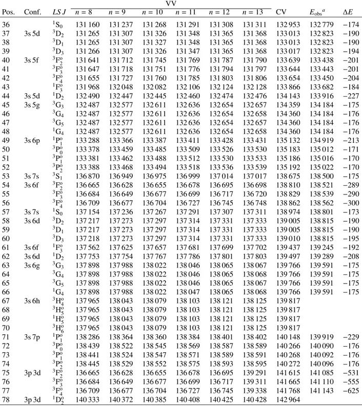
4.2. Al II
In Table A.1, the computed excitation energies, based on VV correlation, are given as a function of the increasing active set of orbitals. When adding the n= 12 correlation layer, the values for all computed energy separations have converged. The agree-ment with the NIST observed energies (Kramida et al. 2018) is, at this point, fairly good. The mean relative difference between theory and experiment is of the order of 1.2%. However, when accounting for CV correlation, the agreement with the observed values is significantly improved, resulting in a mean relative dif-ference being less than 0.2%. Accounting for CV effects also results in a labelling of the eigenstates that matches observations. For instance, when only VV correlation is taken into account, the3F triplet with the highest energy is labelled as a 3s6f level.
After taking CV effects into account, the eigenstates of this triplet are assigned the 3p3d configuration, now the one with the largest expansion coefficient, which agrees with observa-tions. There are no experimental excitation energies for the sin-glet and triplet 3s6h1,3Hterms. In the last column of TableA.1, the differences ∆E between computed and observed energies are displayed. All ∆E values maintain the same sign, being negative.
In Table3, a comparison between the present computed exci-tation energies and those from the MCHF-BP calculations by Froese Fischer et al.(2006) is also performed for Al ii. The latter spectrum calculations are extended up to levels corresponding to the singlet 3p2 1S state and all types of correlation, i.e. VV, CV,
and CC, were accounted for. Both computational approaches are highly accurate, yet the majority of the levels is better repre-sented by the current RCI results. The average relative di ffer-ence for the RCI values is ∼0.2% and for the MCHF-BP ∼0.3%. Moreover, the ∆EMCHF−BP values do not always maintain the
same sign, while the ∆ERCI values do. Hence, in general, the
MCHF-BP calculations do not predict the transition energies as precisely as the present RCI method.
For all computed E1 transitions in Al ii, transition data tables can also be found at the CDS. In Table 4, a statistical analy-sis of the uncertainties to the computed transition rates ARCI is
performed in a similar way to that for Al i. The transitions are also arranged here in four groups. Following the conclusions by Pehlivan Rhodin et al. (2017) and Pehlivan Rhodin (2018), the transitions involving any of the 3s7p1,3P states have been excluded from this analysis. The discrepancies between the length and velocity forms for transitions including the 3s7p1,3P states are consistently large, and thus the computed transition rates are not trustworthy. We note that overall the average uncer-tainty, as well as the value that includes 75% of the data, appear to be smaller, for each group of transitions, than the predicted values in Al i. Nevertheless, the maximum values of the uncer-tainties for the last two groups are larger in comparison to Al i. This is due to some transitions involving 3p3d3F as the upper level. The strong mixing between the 3p3d3F and the 3s6f3F
levels results in strong cancellation effects. Such effects often
hamper the accuracy of the computed transition data and result in large discrepancies between the length and velocity forms.
In Table 7, current RCI theoretical transition rates are compared with the values from the MCHF-BP calculations byFroese Fischer et al.(2006) and, whenever available, results from the B-spline configuration interaction (BSCI) calcula-tions by Chang & Fang (1995). For the majority of the tran-sitions, there is an excellent agreement between the RCI and MCHF-BP values with the relative difference being less than 1%. Some of the largest discrepancies are observed for the 3s3d, 3p2 1D → 3s3p1,3Po transitions. According to
Froese Fischer et al. (2006), correlation is extremely important for transitions from such1D states. In the MCHF-BP
calcula-tions, all three types of correlation, i.e. VV, CV, and CC, have been accounted for; however, the CSF expansions obtained from SD-substitutions are not as large as in the present calculations and the LS -composition of the configurations might not be pre-dicted as accurately. Hence, the evaluation of line strengths for transitions involving 1D states and in turn the computation of transition rates involving these states will be affected. Com-puted transition rates using the BSCI approach are provided for transitions that involve only singlet states. The BSCI cal-culations do not account for the relativistic interaction and no separate values are given for the different fine-structure com-ponents of triplet states. For the 3p2 1D → 3s3p1Potransition,
the discrepancy between the RCI and BSCI values is also quite large. On the other hand, for the 3s3d1D → 3s3p1Po
transi-tion, the BSCI result is in perfect agreement with the present ARCI value. The agreement between the current RCI and BSCI
transition rates exhibits a broad variation. The advantage of the BSCI approach is that it takes into account the effect of the positive-energy continuum orbitals in an explicit manner. Never-theless, the parametrized model potential that is being used in the work byChang & Fang(1995) is not sufficient to describe states that are strongly mixed. Finally, we note the discrepancy for the 3s4p1Po → 3s2 1S
0transition, which is quite large between the
RCI and MCHF-BP values and inexplicably large between the RCI and BSCI values.
In singly ionized aluminium, measurements of transition properties are available only for a few transitions. In Table7, the available experimental results are compared with the the-oretical results from the current RCI calculations, and with the former calculations by Froese Fischer et al. (2006) and Chang & Fang (1995). Transition rates have been experimen-tally observed for the 3s3p1,3Po
1 → 3s
2 1S
0 transitions in the
works by Kernahan et al. (1979), Smith (1970), Berry et al. (1970) andHead et al.(1976), and byTräbert et al.(1999) and Johnson et al.(1986), respectively. In Table7, the average value of these works is displayed. The agreement with the current RCI results is fairly good. Nonetheless, the averaged Aobs by
Träbert et al.(1999) andJohnson et al.(1986) is in better agree-ment with the value byFroese Fischer et al.(2006). Additionally, Vujnovi´c et al.(2002) provided experimental transition rates for the 3p2 1D
2 → 3s3p1P1 and 3p2 1D2 → 3s3p3P1,2transitions
by measuring relative intensities of spectral lines. These experi-mental results, however, differ from the theoretical values.
In the last portion of Table 7, current rates for transitions between states with higher energies are compared with the results from the close coupling (CC) calculations byButler et al. (1993) and the early results from the configuration interaction (CI) calculations byChang & Wang(1987). The results from the latter two calculations are found to be in very good agreement. Furthermore, the agreement between the RCI results and those from the CC and CI calculations is also very good
Table 7. Comparison between computed and observed transition rates A in s−1
for selected transitions in Al ii.
Upper Lower ARCIa Atheorb,c Atheore, f Aobsd,h,g
3s3p3Po 1 3s
2 1S
0 3.054E+03 3.277E+03b 3.30E+03h
3s3p1Po 1 3s
2 1S
0 1.404E+09 1.400E+09b 1.486E+09f 1.45E+09g
3s4s3S 1 3s3p3Po0 8.612E+07 8.572E+07b 3s3p3Po 1 2.555E+08 2.547E+08 b 3s3p3Po 2 4.173E+08 4.162E+08 b 3s4s1S 0 3s3p1Po1 3.422E+08 3.455E+08 b 3.408E+08f 3p2 1D 2 3s3p1Po1 2.523E+05 3.804E+05 b 3.980E+05f 1.84E+04d 3s3p3Po 1 1.790E+04 2.016E+04 b 0.19E+04d 3s3p3Po 2 2.827E+04 3.141E+04 b 0.30E+04d 3p2 3P 0 3s3p3Po1 1.236E+09 1.235E+09b 3p2 3P 1 3s3p3Po0 4.148E+08 4.144E+08 b 3s3p3Po 1 3.058E+08 3.062E+08 b 3s3p3Po 2 5.170E+08 5.167E+08 b 3p2 3P 2 3s3p3Po1 3.145E+08 3.144E+08 b 3s3p3Po 2 9.264E+08 9.272E+08 b 3p2 1S 0 3s3p1Po1 1.020E+09 6.738E+08 b 3s3p3Po 1 5.021E+08 3.399E+07 b 3s3d3D 2 3s3p3Po1 8.977E+08 9.072E+08 b 3s3p3Po 2 3.019E+08 3.046E+08 b 3s3d3D 3 3s3p3Po2 1.197E+09 1.208E+09 b 3s3d1D 2 3s3p1Po1 1.388E+09 1.429E+09 b 1.388E+09f 3s4p3Po 0 3s4s 3S 1 5.639E+07 5.705E+07b 3s3d3D 1 1.556E+07 1.520E+07b 3s4p3Po 1 3s4s 3S 1 5.649E+07 5.724E+07b 3s3d3D 1 3.905E+06 3.816E+06b 3s3d3D 2 1.172E+07 1.146E+07b 3s4p3Po 2 3s4s 3S 1 5.683E+07 5.762E+07b 3s3d3D 1 1.568E+05 1.541E+05b 3s3d3D 2 2.361E+06 2.312E+06b 3s3d3D 3 1.319E+07 1.294E+07b 3s4p1Po 1 3s 2 1S
0 1.527E+06 0.981E+06b 5.079E+06f
3p2 1D
2 5.835E+07 5.897E+07b 6.307E+07f
3s4s1S
0 3.109E+07 2.965E+07b 3.111E+07f
3p3d3Fo 2 3s3d
3D
1 2.956E+08 2.07E+08c 2.14E+08e
3p3d3Fo 3 3s3d
3D
2 3.174E+08 2.19E+08c 2.25E+08e
3p3d3Fo 4 3s3d
3D
3 3.794E+08 2.47E+08c 2.54E+08e
3s4f3Fo 2 3s3d
3D
1 1.981E+08 1.97E+08c 1.98E+08e
3s4f3Fo 3 3s3d
3D
2 2.096E+08 2.09E+08c 2.07E+08e
3s4f3Fo 4 3s3d
3D
3 2.360E+08 2.35E+08c 2.33E+08e
3s5f3Fo 2 3s3d
3D
1 2.801E+07 2.40E+07c 2.50E+07e
3s5f3Fo 4 3s3d
3D
3 3.438E+07 2.85E+07c 2.90E+07e
3s6f3Fo 2 3s3d
3D
1 1.957E+07 2.90E+07c 3.10E+07e
3s4d3D
1 1.116E+07 1.07E+07c 1.00E+07e
3s6f3Fo 3 3s3d
3D
2 1.910E+07 3.07E+07c 3.30E+07e
3s4d3D
2 1.200E+07 1.14E+07c 1.10E+07e
3s6f3Fo 4 3s3d
3D
3 1.920E+07 3.46E+07c 3.70E+07e
3s4d3D
3 1.367E+07 1.28E+07c 1.20E+07e
Notes. The present values from the RCI calculations are given in Col. 3. In the next two columns, theoretical values from former MCHF-BP, close coupling (CC), configuration interaction (CI), and B-spline configuration interaction (BSCI) calculations are given. The last column contains the results from experimental observations. All theoretical transition rates are presented in length form.
References. (a)Present calculations; (b)Froese Fischer et al. (2006); (c)Butler et al. (1993); (d)Vujnovi´c et al. (2002); (e)Chang & Wang (1987); ( f )Chang & Fang(1995); (g)Kernahan et al.(1979),Smith(1970),Berry et al.(1970),Head et al.(1976);(h)Träbert et al.(1999),Johnson et al.
(1986).
for the 3s4f3F → 3s3d3D transitions and fairly good for the 3s5f3F → 3s3d3D transitions. On the other hand, for
the 3p3d, 3s6f3F → 3s3d3D transitions, the observed discrep-ancy between the current RCI values and those from the two
pre-vious calculations is substantial. This outcome indicates that the calculations byButler et al. (1993) and Chang & Wang(1987) are insufficient to properly account for correlation and further emphasizes the quality of the present work.
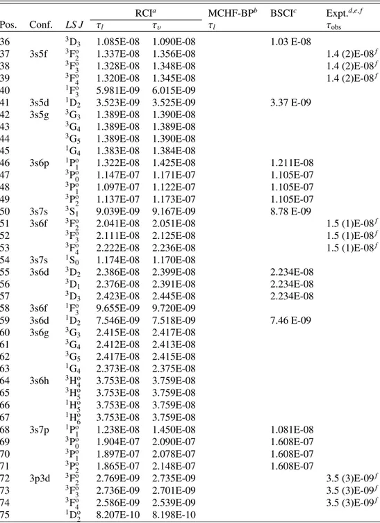
In the same way as for Al i, the lifetimes of Al ii excited states were also estimated based on the computed E1 transitions. In TableA.2, both length τl and velocity τυ forms of the
cur-rently computed lifetimes are displayed. As already mentioned, the agreement between these two forms serves as an indica-tion of the quality of the results. The average relative difference between the two forms is ∼2%. The largest discrepancies are observed between the length and velocity gauges of the singlet 3p2 1D state, and between the singlet and triplet 3s7p1,3P states.
The highest computed levels in the calculations of Al ii corre-spond to configuration states with orbitals up to n = 7, such as 3s7p. Similarly to the conclusions for the lifetimes of Al i, better agreement between the length and velocity forms of the 3s7p1,3P states could probably be obtained by including 3snl
configurations with n > 7 in the MR.
In TableA.2, the lifetimes from the current RCI calculations are compared with results from previous MCHF-BP and BSCI calculations byFroese Fischer et al. (2006) andChang & Fang (1995), respectively. Except for the lifetimes of the triplet 3s3p3Po
1and singlet 3p
2 1D
2states, the agreement between the
RCI and MCHF-BP calculations is very good. Furthermore, the overall agreement between the RCI and BSCI calculations is suf-ficiently good. Despite the poor agreement between the RCI and BSCI values for the 3p2 1D2and 3s7p1,3P states, for the rest of
the states the discrepancies are small. The BSCI results are more extended. However, no separate values are provided for the dif-ferent LS J-components of the triplet states and the average life-time is presented for them instead.
In Table A.2, the theoretical lifetimes are also com-pared with available measurements. The measured lifetime of the 3s3p3Po1 state by Träbert et al. (1999) and Johnson et al. (1986) agrees remarkably well with the calculated value by Froese Fischer et al. (2006). The agreement with the current results is fairly good too. The lifetime of the 3s3p1Po
1state
mea-sured byKernahan et al.(1979),Head et al.(1976),Berry et al. (1970), andSmith(1970) is well represented by all theoretical values. On the other hand, the results from the measurements of the 3snf3F states byAndersen et al.(1971) differ substantially from the theoretical RCI values. For the 3snf3F Rydberg series,
only theoretical lifetimes using the current MCDHF and RCI approach are available. Given the large uncertainties associated with early beam-foil measurements, the discrepancies between theoretical and experimental values are in some way expected. The only exception is the lifetime of the 3s5f3F state, which
is in rather good agreement with the RCI values. In the experi-ments byAndersen et al.(1971) the different fine-structure com-ponents have not been separated and a single value is provided for all three different LS J-levels.
5. Summary and conclusions
In the present work, updated and extended transition data and lifetimes are made available for both Al i and Al ii. The compu-tations of transition properties in these two systems are challeng-ing mainly due to the strong two-electron interaction between the 3s3d1D and 3p2 1D states, which dominates the lowest part of their spectra. Thus, some of the states are strongly mixed and highly correlated wave functions are needed to accurately pre-dict their LS -composition. We are confident that in this work enough correlation has been included to affirm the reliability of the results. The predicted excitation energies are in excel-lent agreement with the experimental data provided by the NIST database, which is a good indicator of the quality of the produced transition data and lifetimes.
We have performed an extensive comparison of the com-puted transition rates and lifetimes with the most recent theoretical and experimental results. There is a significant improvement in accuracy, in particular for the more complex system of neutral Al i. The computed lifetimes of Al i are in very good agreement with the measured lifetimes in high-precision laser spectroscopy experiments. The same holds for the mea-sured lifetimes of Al ii in ion storage rings. The present calcula-tions are extended to higher energies and many of the computed transitions fall in the infrared spectral region. The new genera-tion of telescopes are designed for this region and these transi-tion data are of high importance. The objective of this work is to make available atomic data that could be used to improve the interpretation of abundances in stars. Lists of trustworthy ele-mental abundances will permit the tracing of stellar evolution, as well as the formation and chemical evolution of the Milky Way.
The agreement between the length and velocity gauges of the transition operator serves as a criterion for the quality of the transition data and for the lifetimes. For most of the strong transitions in both Al i and Al ii, the agreement between the two gauges is very good. For transitions involving states with the highest n quantum number for the s and p symmetries, we observe that the agreement between the length and veloc-ity forms is not as good. This becomes more evident when esti-mating lifetimes of excited levels that are associated with those transitions.
Acknowledgements. The authors have been supported by the Swedish Research Council (VR) under contract 2015-04842. The authors acknowledge H. Hartman, Malmö University, and H. Jönsson, Lund University, for discussions.
References
Adibekyan, V. Z., Sousa, S. G., Santos, N. C., et al. 2012,A&A, 545, A32 Andersen, T., Roberts, J. R., & Sørensen, G. 1971,Phys. Scr., 4, 52 Bensby, T., Feltzing, S., & Oey, M. S. 2014,A&A, 562, A71 Berry, H. G., Bromander, J., & Buchta, R. 1970,Phys. Scr., 1, 181 Butler, K., Mendoza, C., & Zeippen, C. 1993,J. Phys. B, 26, 4409 Buurman, E., & Dönszelmann, A. 1990,A&A, 227, 289
Buurman, E., Dönszelmann, A., Hansen, J. E., & Snoek, C. 1986,A&A, 164, 224
Carretta, E., Bragaglia, A., Gratton, R. G., et al. 2010,A&A, 516, A55 Chang, T. N., & Fang, T. K. 1995,Phys. Rev. A, 52, 2638
Chang, T. N., & Wang, R. 1987,Phys. Rev. A, 36, 3535
Clayton, D. D. 2003,Handbook of Isotopes in the Cosmos: Hydrogen to Gallium (Cambridge: Cambridge University Press)
Davidson, M. D., Volten, H., & Dönszelmann, A. 1990,A&A, 238, 452 Dyall, K. G., Grant, I. P., Johnson, C., Parpia, F. A., & Plummer, E. P. 1989,
Comput. Phys. Commun., 55, 425
Ekman, J., Godefroid, M., & Hartman, H. 2014,Atoms, 2, 215 Froese Fischer, C. 2009,Phys. Scr., T134, 014019
Froese Fischer, C., Tachiev, G., & Irimia, A. 2006,At. Data Nucl. Data Tables, 92, 607
Froese Fischer, C., Godefroid, M., Brage, T., Jönsson, P., & Gaigalas, G. 2016, J. Phys. B: At. Mol. Opt. Phys., 49, 182004
Gaigalas, G., Rudzikas, Z., & Froese Fischer, C. 1997,J. Phys. B: At. Mol. Opt. Phys., 30, 3747
Gaigalas, G., Fritzsche, S., & Grant, I. P. 2001,Comput. Phys. Commun., 139, 263
Gaigalas, G., Zalandauskas, T., & Rudzikas, Z. 2003,At. Data Nucl. Data Tables, 84, 99
Gaigalas, G., Zalandauskas, T., & Fritzsche, S. 2004,Comput. Phys. Commun., 157, 239
Gaigalas, G., Froese Fischer, C., Rynkun, P., & Jönsson, P. 2017,Atoms, 5, 6 Gehren, T., Liang, Y. C., Shi, J. R., Zhang, H. W., & Zhao, G. 2004,A&A, 413,
1045
Gehren, T., Shi, J. R., Zhang, H. W., Zhao, G., & Korn, A. J. 2006,A&A, 451, 1065
Grant, I. P. 2007, Relativistic Quantum Theory of Atoms and Molecules (New York: Springer)
Head, M. E. M., Head, C. E., & Lawrence, J. N. 1976, inAtomic Structure and Lifetimes, eds. F. A. Sellin, & D. J. Pegg (NY: Plenum),147
Hibbert, A. 1989,Phys. Scr., 39, 574
Jönsson, G., & Lundberg, H. 1983,Z. Phys. A, 313, 151
Johnson, B. C., Smith, P. L., & Parkinson, W. H. 1986,ApJ, 308, 1013 Jönsson, G., Kröll, S., Persson, A., & Svanberg, S. 1984,Phys. Rev. A, 30,
2429
Jönsson, P., Gaigalas, G., Biero´n, J., Froese Fischer, C., & Grant, I. P. 2013,Phys. Commun., 184, 2197
Kelleher, D. E., & Podobedova, L. I. 2008a,J. Phys. Chem. Ref. Data, 37, 709 Kelleher, D. E., & Podobedova, L. I. 2008b,J. Phys. Chem. Ref. Data, 37, 267 Kernahan, J. A., Pinnington, E. H., O’Neill, J. A. M., Brooks, R. L., & Donnely,
K. E. 1979,Phys. Scrip., 19, 267
Kramida, A., Ralchenko, Y. u., & Reader, J. NIST ASD Team 2018,NIST Atomic Spectra Database, ver. 5.5.3 (Online), available: https://physics. nist.gov/asd (2018, March 15), National Institute of Standards and Technology, Gaithersburg, MD
Lin, C. D. 1974,ApJ, 187, 385
McKenzie, B. J., Grant, I. P., & Norrington, P. H. 1980,Comput. Phys. Commun., 21, 233
Mendoza, C., Eissner, W., Le Dourneuf, M., & Zeippen, C. J. 1995,J. Phys. B, 28, 3485
Mishenina, T. V., Soubiran, C., Bienaymé, O., et al. 2008,A&A, 489, 923
Nordlander, T., & Lind, K. 2017,A&A, 607, A75
Olsen, J., Roos, B. O., Jorgensen, P., & Jensen, H. J. A. a. 1988,J. Chem. Phys., 89, 2185
Pehlivan Rhodin, A., Hartman, H., Nilsson, H., & Jönsson, P. 2017,A&A, 598, A102
Pehlivan Rhodin, A. 2018, Ph. D. Thesis, Lund Observatory
Reddy, B. E., Lambert, D. L., & Allende Prieto, C. 2006,MNRAS, 367, 1329 Smiljanic, R., Korn, A. J., Bergemann, M., Frasca, A., et al. 2014,A&A, 570,
A122
Smiljanic, R., Romano, D., Bragaglia, A., Donati, P., et al. 2016,A&A, 589, A115
Smith, W. H. 1970,NIM, 90, 115
Sturesson, L., Jönsson, P., & Fischer, C. F. 2007,Comput. Phys. Commun., 177, 539
Tayal, S. S., & Hibbert, A. 1984,J. Phys. B, 17, 3835
Taylor, P. R. C. W., Bauschlicher, J., & Langhoff, S. 1988,J. Phys. B, 21, L333 Theodosiou, C. E. 1992,Phys. Rev. A, 45, 7756
Trefftz, E. 1988,J. Phys. B: At. Mol. Opt. Phys., 21, 1761 Träbert, E., Wolf, A., & Linkemann, J. 1999,J. Phys. B, 32, 637
Vujnovi´c, V., Blagoev, K., Fürböck, C., Neger, T., & Jäger, H. 2002,A&A, 338, 704
Weiss, A. W. 1974,Phys. Rev., 9, 1524
Wiese, W. L., Smith, M. W., & Miles, B. M. 1969,NSRDS-NBS, 22, 47 Wiese, W. L., & Martin, G. A. 1980, inTransition Probabilities, Part II, Vol. Natl.
Appendix A: Additional tables
Table A.1. Computed excitation energies in cm−1
for the 78 lowest states in Al ii.
VV
Pos. Conf. LS J n= 8 n= 9 n= 10 n= 11 n= 12 n= 13 CV Eobsa ∆E
1 3s2 1S 0 0 0 0 0 0 0 0 0 0 2 3s 3p 3Po0 36 227 36 280 36 298 36 318 36 332 36 335 37 445 37 393 −52 3 3Po 1 36 286 36 339 36 357 36 377 36 391 36 394 37 503 37 454 −49 4 3Po2 36 405 36 459 36 477 36 496 36 511 36 514 37 626 37 578 −48 5 1Po 1 59 810 59 698 59 617 59 619 59 606 59 602 59 982 59 852 −130 6 3p2 1D2 83 542 83 596 83 620 83 641 83 657 83 660 85 692 85 481 −211 7 3s 4s 3S 1 89 965 90 028 90 059 90 082 90 099 90 102 91 425 91 275 −150 8 3p2 3P 0 92 679 92 709 92 716 92 736 92 750 92 752 94 211 94 085 −126 9 3P1 92 739 92 769 92 776 92 795 92 809 92 812 94 264 94 147 −117 10 3P 2 92 855 92 885 92 892 92 912 92 926 92 928 94 375 94 269 −106 11 3s 4s 1S0 94 003 94 057 94 084 94 101 94 111 94 114 95 543 95 351 −192 12 3s 3d 3D 2 94 262 94 243 94 241 94 262 94 278 94 280 95 791 95 549 −242 13 3D 1 94 261 94 243 94 242 94 263 94 279 94 281 95 794 95 551 −243 14 3D3 94 263 94 242 94 239 94 261 94 276 94 279 95 804 95 551 −253 15 3s 4p 3Po 0 103 935 104 003 104 030 104 053 104 070 104 073 105 582 105 428 −154 16 3Po1 103 948 104 017 104 044 104 067 104 084 104 087 105 594 105 442 −152 17 3Po 2 103 976 104 045 104 073 104 095 104 112 104 115 105 623 105 471 −152 18 1Po 1 105 597 105 643 105 655 105 673 105 683 105 685 107 132 106 921 −211 19 3s 3d 1D 2 109 010 108 919 108 897 108 910 108 918 108 918 110 330 110 090 −240 20 3p2 1S 0 111 100 110 804 110 659 110 643 110 618 110 608 112 086 111 637 −449 21 3s 5s 3S1 118 564 118 632 118 661 118 685 118 702 118 705 120 259 120 093 −166 22 1S 0 119 807 119 878 119 908 119 931 119 946 119 948 121 544 121 367 −177 23 3s 4d 3D 2 120 013 120 034 120 045 120 068 120 085 120 088 121 684 121 484 −200 24 3D1 120 013 120 034 120 046 120 068 120 085 120 088 121 685 121 484 −201 25 3D 3 120 014 120 034 120 045 120 068 120 084 120 087 121 688 121 484 −204 26 3s 4f 3Fo 2 121 657 121 739 121 772 121 797 121 815 121 818 123 606 123 418 −188 27 3Fo3 121 659 121 742 121 775 121 799 121 817 121 820 123 608 123 420 −188 28 3Fo 4 121 663 121 745 121 778 121 802 121 820 121 824 123 612 123 423 −189 29 1Fo 3 121 735 121 818 121 852 121 876 121 894 121 898 123 657 123 471 −186 30 3s 4d 1D2 123 606 123 489 123 461 123 473 123 482 123 483 125 049 124 794 −255 31 3s 5p 3Po0 124 108 124 185 124 212 124 236 124 254 124 257 125 869 125 703 −166 32 3Po 1 124 114 124 190 124 218 124 242 124 259 124 262 125 874 125 709 −165 33 3Po 2 124 126 124 203 124 231 124 254 124 272 124 275 125 887 125 722 −165 34 1Po 1 124 302 124 375 124 401 124 424 124 440 124 443 126 078 125 869 −209 35 3s 6s 3S1 130 615 130 689 130 716 130 740 130 758 130 761 132 386 132 216 −170
Notes. The energies are given as a function of the increasing active set of orbitals, accounting for VV correlation, where n indicates the maximum principle quantum number of the orbitals included in the active set. In Col. 10, the final energy values are displayed after accounting for CV correlation. The differences ∆E between the final computations and the observed values are shown in the last column. The sequence and naming of the configurations and LS J-levels are in accordance with the final (CV) computed energies. The levels of the singlet and triplet 3s6h1,3H and
the 3p3d1D level have not yet been observed, and so the∆E values are not available.