(will be inserted by the editor)
A Method for Evaluation of Learning Components
Niklas Lavesson · Veselka Boeva · Elena Tsiporkova · Paul Davidsson
Received: date / Accepted: date
Abstract Today, it is common to include machine learning components in software products. These components offer specific functionalities such as image recogni-tion, time series analysis, and forecasting but may not satisfy the non-functional constraints of the software products. It is difficult to identify suitable learning algo-rithms for a particular task and software product because the non-functional require-ments of the product affect algorithm suitability. A particular suitability evaluation may thus require the assessment of multiple criteria to analyse trade-offs between functional and non-functional requirements. For this purpose, we present a method for APPlication-Oriented Validation and Evaluation (APPrOVE). This method com-prises four sequential steps that address the stated evaluation problem. The method provides a common ground for different stakeholders and enables a multi-expert and multi-criteria evaluation of machine learning algorithms prior to inclusion in software products. Essentially, the problem addressed in this article concerns how to choose the appropriate machine learning component for a particular software product Keywords Data Mining · Evaluation · Machine Learning
N. Lavesson
Blekinge Institute of Technology, SE–371 79 Karlskrona, Sweden Tel.: +46-455-385875, Fax: +46-455-385057
E-mail: Niklas.Lavesson@bth.se V. Boeva
Technical University of Sofia, branch Plovdiv
Computer Systems and Technologies Department, Plovdiv, Bulgaria E-mail: vboeva@tu-plovdiv.bg
E. Tsiporkova
Software Engineering and ICT group
Sirris, The Collective Center for the Belgian Technological Industry Brussels, Belgium
E-mail: elena.tsiporkova@sirris.be P. Davidsson
Malm¨o University, SE–205 06 Malm¨o, Sweden E-mail: Paul.Davidsson@mah.se
1 Introduction
Many software products feature machine learning or adaptive components. These components offer specific functionalities to the software products but the components may not satisfy the non-functional requirements of the software product. It is com-mon to evaluate computational efficiency and accuracy machine learning research but these performance measures are seldom traded off and other criteria are usually ignored (Japkowicz and Shah, 2011). This method of evaluation is insufficient if the goal is to determine algorithm suitability for a particular task and software product when there are multiple non-functional constraints to satisfy and multiple stakehold-ers involved. This article presents a four-step method for this purpose. We denote the method APPlication-Oriented Validation and Evaluation (APPrOVE). The APPrOVE method is targeted towards multi-expert and multi-criteria evaluation of unsupervised and supervised learning algorithms.
1.1 Aim and Scope
The problem addressed in this article concerns how to choose the appropriate ma-chine learning component for a particular software product. To address this problem, the aim is to present and analyse a method for multi-expert and multi-criteria evalu-ation of learning algorithms. The objectives are to motivate the steps that constitute the method and to review and demonstrate each step. The scope is limited to two supervised learning cases but the method is generic and should be applicable to any supervised or unsupervised learning context. The main contribution of this article is the method description and review. In addition, the article also includes an analysis of two alternative evaluation criteria prioritisation methods.
1.2 Outline
The remainder of the article is organised as follows: in Section 2, we provide an analysis of the machine learning evaluation and review related work. The APPrOVE method is presented in Section 3. In Section 4 and Section 5, we present two case studies where the method is applied for evaluation. Section 7 covers conclusions and pointers to future work.
2 Background
Real-world applications and software products often feature space and time require-ments. As a consequence, some algorithms are unsuitable when test sets are ex-tremely large or where storage space or computational power is very limited (Bucila et al, 2006). Thus, in order to select appropriate classifiers or algorithms for such applications we must evaluate performance in terms of space and time. We make a distinction between criteria and metrics in that the latter are used to evaluate the
former. Accuracy, space, and time could all be regarded as sub criteria of the perfor-mance criterion but it makes sense to discuss these sub-criteria explicitly as distinct criteria because the term performance is frequently used to denote accuracy.
If the goal is to discover new knowledge to be used in human decision making there might be completely different criteria to consider in addition to performance. For example, comprehensibility may relate to how well we understand the classi-fier and the decision process. In addition, a crucial aspect of data mining is that the discovered knowledge should be somehow interesting. This is related to the interest-ingness criterion (Freitas, 1998), which has to do with the unexpectedness, usefulness and novelty of the discovered knowledge. Comprehensibility may also be associated with complexity (Gaines, 1996) in that an intricate or complex model is intuitively more difficult to comprehend than a simple model.
We have now highlighted some examples of criteria that can be important to eval-uate but we believe there are many more to consider for various domains. As a con-sequence, we argue that evaluation criteria should be selected on the basis of the problem at hand. Moreover, it seems plausible that one should first decide on what criteria to evaluate before selecting metrics. This might sound obvious, but many studies seem to assume that accuracy is the only criterion worth evaluating (Provost et al, 1998).
Arguably, there is a need for; (i) common definitions of relevant evaluation cri-teria and (ii) systematic approaches to associate cricri-teria with suitable metrics. The requirements of real-world applications often imply that a suitable trade-off between several important criteria is desired. For example, it has been noted that the accuracy and comprehensibility of rules are often in conflict with each other (Freitas, 1998). Thus, depending on the application, the evaluation may involve trading off multi-ple criteria. Since metrics are used to evaluate criteria, this means that a systematic approach is needed to trade off multiple metrics for these cases.
We believe that there is a fundamental problem associated with some of the pro-posed multi-criteria metrics for classifier evaluation in that they are usually based on a static set of metrics. As discussed by Lavesson and Davidsson (2008), one study proposes the SAR metric, which combines squared error, success rate, and the area under the ROC curve. This metric may very well be quite suitable for a certain ap-plication, however, it cannot be used to compare any other criteria than classification performance.
Thus, we need a standardised way to trade off multiple metrics but, at the same time, we would like the actual choice of which metrics to include to be made on the basis of the requirements and characteristics of the particular application at hand. We therefore suggest the use of Generic Multi-Criteria (GMC) metrics, which dictate how to integrate metrics but do not specify which metrics to include.
It could be argued that there is no need for GMC metrics and that the integration could instead be tailor-made for the application at hand. However, we argue that one of the main benefits that stem from using a GMC metric is that different instances of such a metric could be more easily compared and refined across studies and ap-plications. In addition, the use of a GMC metric automatically shifts the focus from integration issues to application issues. The GMC metric approach also simplifies the development and use of what we refer to as metric-based learning algorithms, that is,
algorithms that take a metric as input and try to learn a classifier with optimal perfor-mance with respect to this metric. A metric-based algorithm that is based on a GMC metric can thus be tailored for a particular application by selecting relevant metrics and specifying trade-offs.
We have discussed several aspects of application-oriented evaluation and would like to stress the importance of understanding the characteristics, requirements, re-strictions, goals, and the context of the application to be able to properly select suit-able criteria and metrics and to define meaningful trade-offs. Unfortunately, these aspects are covered in an ad-hoc manner by many studies if covered at all (Japkowicz and Shah, 2011).
2.1 Related Work
A few studies address user-oriented and application-oriented evaluation of classifiers and learning algorithms. For example, Nakhaeizadeh and Schnabl (1997) present a multi-criteria metric for learning algorithm evaluation and define the efficiency of an algorithm as its weighted positive properties (for example, understandability) di-vided by its weighted negative properties (for example, computation time). The met-ric weights for the efficiency metmet-ric are decided by an optimisation algorithm in order to calculate objective weights. One problem with this approach is that these objective weights might not contribute to a realistic representation of the studied application. In a follow-up paper, Nakhaeizadeh and Schnabl (1998) also suggest an approach for measuring qualitative properties, such as understandability, using the efficiency met-ric. In addition, a personalised algorithm evaluation is introduced, which is basically a collection of approaches to specify user preferences about restrictions and accept-able ranges on different metrics. The personalised evaluation approaches enaccept-able the user to influence the weights to reflect, for example, that understandability is more important than accuracy. However, one of the main problems is that the user prefer-ences are defined as linear equalities of inputs and outputs. The paper features some discussion on how to quantify qualitative metrics, however, no information is given about how to select relevant metrics.
Lavesson and Davidsson (2010) present the first generation of the APPrOVE method as a means for conducting systematic application-oriented evaluation of clas-sifiers and learning algorithms. The first generation of APPrOVE is focused on the core ideas to represent evaluation criteria as quality attributes and to follow a struc-tured process in which the application at hand is described, quality attributes are identified, each attribute is associated with one or more evaluation metrics, and the selected metrics are integrated into a multi-metric which can be used to rank or just assess the quality of algorithms and classifiers. However, the first generation of AP-PrOVE lacks several important components, for example: the formal inclusion of the roles of stakeholders and domain experts, and the formal means to make a group-based decision or assessment, group-based on input from those roles.
Except for the initial APPrOVE study there exist few systematic approaches to evaluate learning algorithms according to multiple criteria and on the basis of a par-ticular application. In a recent book on the topic of machine learning evaluation,
Japkowicz and Shah (2011) present a comprehensive description of the state-of-the-art and describe a framework for evaluating learning algorithms. Although the book focuses on predictive performance, the authors mention the possibility to evaluate comprehensibility and interestingness as an alternative means of evaluation. With re-gard to analysis and evaluation of prediction systems in software engineering, the Journal of Empirical Software Engineering recently featured a special issue on the topic of repeatable results in software engineering prediction. Menzies and Shep-perd (2012) believe that conclusion instability (i.e., what is concluded as true for one project or case study is concluded as false for another project or case study) is en-demic within software engineering. Menzies and Shepperd (2012) describe different reasons for the occurrence of conclusion instability and sketch a number of ideas for reducing conclusion instability. Many of these ideas are also discussed in the context of evaluation in the data mining and machine learning communities (cf., Japkowicz and Shah (2011)).
We are unable to find any applicable published work on expert and multi-criteria evaluation methods for machine learning components.
3 The APPrOVE Method
The extension of the APPrOVE method in a multi-expert context as introduced here has been inspired by a work on collaborative decision making (Tsiporkova et al, 2010). The latter proposes a collaborative decision support platform which supports the product manager in defining the contents of a product release and allows inter-active and collaborative decision making by facilitating the exchange of information about product features among individual autonomous stakeholders.
APPrOVE is based on concepts from software engineering. It is therefore bene-ficial to begin the description of the method by introducing three interrelated defini-tions. Firstly, given that we regard a learning algorithm (or a classifier) as an item: Definition 1 A quality attribute is a feature or characteristic that affects an item’s quality1.
In order for Definition 1 to be meaningful in the application-oriented evaluation con-text, we also define the meaning of quality as it pertains to such an item:
Definition 2 Quality is the degree to which a component, system or process meets specified requirements and/or user/customer needs and expectations2.
Commonly and intuitively, quality attributes are evaluated using quality metrics. For our purposes, the following definition of metrics is applicable:
Definition 3 A metric is a measurement scale and the method used for measurement
3.
1 IEEE Standard Glossary of Software Engineering Terminology
2 IEEE Standard Glossary of Software Engineering Terminology
These definitions are fairly straight-forward to comprehend but difficulties arise when it comes to apply the attribute–metric concept in practice. Unlike software engineer-ing, the machine learning and data mining areas of research have not been concerned with the definition of quality attributes or the mapping between quality attributes and quality metrics. As will be described later, we have therefore borrowed definitions from software engineering for quality attributes that are applicable to our context.
The validation of a learning algorithm or a classifier with respect to a certain ap-plication by involving a group of domain experts is a process, which can be divided in two separate phases: i) interaction and evaluation phase engaging individual domain experts ii) validation and decision phase usually performed by the designer/developer. Subsequently, the proposed extension of APPrOVE method consists of two main components: i) The evaluation workspace, which is used by the domain experts to discuss personal opinions and share mutual insights about the quality attributes and metrics. It provides the necessary functionalities to allow an individual domain expert to engage in the evaluation process: attribute prioritising, metric ranking, domain expert rating and metric acceptable range specifying, ii) The validation engine, which implements different algorithms that blend metric scores, quality attribute weights and domain expert weights provided by each individual domain expert into a single group-based evaluation score.
The interaction and evaluation phase is initiated by the designer/developer, who supplies the initial list of quality attributes for the considered application and the corresponding lists of suitable metrics (one or more per attribute), and provides access to the evaluation workspace for all involved domain experts:
– Domain experts use the evaluation component to discuss and identify quality at-tributes for the problem at hand. Each expert can assess the relative importance of each quality attribute in comparison to other attributes.
– Domain experts engage in discussions about metrics and identify how the quality attributes are supposed to be evaluated.
– Each domain expert can use the workspace to specify the acceptable range for each selected metric.
– Each domain expert forms an opinion about other experts, and reflect this by assigning weights to the other experts.
The designer/developer closes the interaction and evaluation phase and enters the validation and decision phaseby launching the validation engine:
– The validation engine is used to calculate the individual metric scores for each domain expert.
– Metric scores, quality attribute weights and domain experts weights provided by each individual domain expert are aggregated into group-based metric scores and consensus attribute weights.
– The ultimate goal of the validation engine is to generate a group-based evaluation score supported by all the domain experts.
3.1 Evaluation Workspace
3.1.1 Identification of Quality Attributes
The process of identifying relevant quality attributes for the problem at hand should be simple. However, quality attributes can be defined at a number of abstraction levels. For example, depending on the characteristics of the problem, one might need to evaluate training-related (algorithmic) properties or testing-related (classifier-specific) properties (Lavesson and Davidsson, 2007). Moreover, some attributes can only be subjectively evaluated while others are associated with objective metrics.
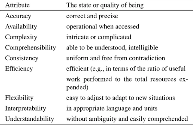
The designer/developer is supposed to supply the initial list of quality attributes, which consists of two separate lists: i) a list of main attributes, which are prelimi-nary identified by the developer/designer to match the (in)formal application require-ments or objectives, ii) a list of complementary attributes, which will be discussed and ranked by the domain experts in order to complement the identified list of main attributes. In order to facilitate the domain experts in the latter task we suggest the use of a list of pairs of quality attributes and concise descriptions as shown in Table 1 where quality attributes correspond concrete qualities.
Let us formally define our attribute selection model. Assume a list of l additional quality attributes is supplied. Then each domain expert is given the possibility to vote for these attributes, thereby expressing his/her own personal view about the attributes’ relevance to the problem at hand. Thus each expert i can vote for the attributes by assigning a binary vector ui= [ui1, . . . , uil], where ui j∈ {0, 1} for i = 1, . . . , k.
Ulti-mately, the matrix k × l will be constructed as a whole:
U= u11. . . u1l .. . ... uk1· · · ukl . Subsequently, each quality attribute satisfying the condition
k
∑
i=1
ui j> c, where j = 1, . . . , l and c ≥ 0
is selected to complement the list of main attributes previously identified. The ratio-nale behind this is that it is sufficient for an attribute to be considered relevant by at least c experts in order to add this attribute to the final attribute list and c is determined for each different case dependent on the available domain experts to participate in the evaluation process.
3.1.2 Selection of Metrics
As described in Section 2, a certain quality attribute may be evaluated using various metrics, depending on the problem at hand. Several aspects need to be taken into account when selecting metrics for a particular quality attribute. For example, some metrics are generic and may be used for all types of supervised algorithms (e.g., success rate, training time) while others are specific to a certain type of algorithm
Table 1 Examples of quality attributes
Attribute The state or quality of being
Accuracy correct and precise
Availability operational when accessed
Complexity intricate or complicated
Comprehensibility able to be understood, intelligible
Consistency uniform and free from contradiction
Efficiency efficient (e.g., in terms of the ratio of useful
work performed to the total resources ex-pended)
Flexibility easy to adjust to adapt to new situations
Interpretability in appropriate language and units
Understandability without ambiguity and easily comprehended
The definitions have been obtained from IEEE Standard Glossary of Software Engineering Terminology, the New Oxford American Dictionary, and from a study on data quality factors by Wang and Strong (1996).
or classifier type (e.g., tree size, rule size). Additionally, some metrics may be more or less reliable depending on the type and distribution of data (e.g., success rate vs. AUC).
The question is how to select a suitable metric for a specific quality attribute when a group of domain experts is involved in the evaluation process. We propose to use the evaluation workspace in order to engage the domain experts in discussions about the identified attributes and eventual metrics that can be applied for their evaluation. For example, a pool of suitable metrics can be provided for each quality attribute and each domain expert can be given the possibility to vote for these metrics, thereby expressing his/her own personal view about the metrics’ relevance to the attribute in question. Then the same rationale as in Section 3.1.1 can be applied, i.e. it is sufficient for a metric to receive at least c votes in order for this metric to be preserved in the final metric list.
3.1.3 Prioritisation of Quality Attributes
Suppose a real-world application of supervised learning is studied and several im-portant quality attributes are identified. It is then improbable that these attributes are of equal importance. In order to take the difference in attribute importance into ac-count in a meaningful manner, a systematic prioritisation of the quality attributes is desirable.
There are quite a few methods available that perform systematic prioritisation. The quantitative multi-criteria and multi-expert validation and evaluation method, which is the final step in the method, makes use of individual metric weights pro-vided by each domain expert. Since each metric is associated with a quality attribute,
these weights can also be regarded as quality attribute weights4. The Analytic Hier-chary Process (Saaty, 1980) was utilised in (Lavesson and Davidsson, 2010) based on its compliance with these requirements as well as its successful use in similar priori-tisation tasks (Vaidya and Kumar, 2004; Wohlin and Andrews, 2003). The Appendix contains a formal description of the Analytic Hierchary Process. In addition, the Large Preference Relation (Fodor and Roubens, 1994; Roubens and Vincke, 1985) is considered as an alternative technique for attribute prioritisation.
Each domain expert is given the possibility to apply a formal prioritisation method of his own choice or just employ his professional intuition in order to perform com-parison of n identified attributes. Thus each expert i needs to provide a vector of weights wi= [wi1, . . . , win], which satisfy the conditions:
n
∑
j=1
wi j= 1 and wi j∈ (0, 1), for i = 1, . . . , k.
These weights are reflecting the individual judgement of each domain expert about the relative importance of the different quality attributes. The following matrix k × n is subsequently composed: W = w11. . . w1n .. . ... wk1· · · wkn .
3.1.4 Specification of Acceptable Ranges
Our multi-criteria and multi-expert evaluation method also expects each metric to have a particular range. Therefore each expert i (i = 1, . . . , k) is allowed to asso-ciate with each selected metric j ( j = 1, . . . , n) an acceptable range, ri j=
h bli j, bui ji. The lower bound, bli j, denotes the least desired acceptable score. Similarly, the upper bound, bui j, denotes the desired score.
3.1.5 Distribution of Weights over Domain Experts
Each domain expert is allowed to rate their fellow experts, thereby expressing the relative degree of influence the expert is inclined to accept from the rest of the group. Thus a vector of weights vi= [vi1, . . . , vik] will be associated with each domain expert,
where
k
∑
j=1
vi j= 1 and vi j∈ (0, 1), for i = 1, . . . , k.
Note that the latter imposes the usage of non-zero weights, which can be interpreted as disallowing the experts to completely ignore colleagues by assigning them zero
4 In the simplest and perhaps most common case, one metric is selected for each identified quality
attribute. However, the presented method as such, is not limited to accomodating this case; in fact, both the method and the applied prioritisation method can handle multiple metrics for each quality attribute.
weights and in this way putting the decision process in a deadlock. The following square matrix k × k is subsequently composed:
V= v11· · · v1k .. . . .. ... vk1· · · vkk .
Note that the elements on the diagonal express the degree of confidence each expert has in the correctness or objectivity of his/hers own judgement with respect to the other domain experts.
3.2 Validation Engine
3.2.1 Calculation of Individual Metric Scores
Let mj denotes the value of selected metric j ( j = 1, . . . , n). Then a metric score
mi jcan be generated for each domain expert i (i = 1, . . . , k) for each metric j ( j =
1, . . . , n) by using the lower and upper bound of the acceptable range provided by the expert: mi j= 1 :mj−b l i j bui j−bl i j > 1 0 :mj−b l i j bu i j−bli j < 0 mj−bli j bu i j−bli j otherwise . (1)
Thus, a vector of individual metric scores mi= [mi1, . . . , min] is assigned to each
ex-pert i (i = 1, . . . , k) and the following matrix k × n is formed as a whole:
M= m11. . . m1n .. . ... mk1· · · mkn .
3.2.2 Calculation of Group-based Metric Scores
The validation engine can be used to transform the matrix of individual-based metric scores M into a vector of group-based metric scores g = [g1, . . . , gn]. Thus each gj,
( j = 1, . . . , n) can be interpreted as the trade-off value, agreed between the individual domain experts, for the score of metric j.
We apply a recursive aggregation process, developed in (Tsiporkova and Boeva, 2004) (see also (Tsiporkova and Boeva, 2006) and (Tsiporkova et al, 2010)), which is based on the weighted mean aggregation. The individual metric scores of matrix M can initially be combined according to the vector of weights vi(i = 1, . . . , k) assigned
by each domain expert. Consequently, a new matrix of metric scores M0, is obtained as follows:
for each i (i = 1 . . . , k) and j ( j = 1, . . . , n). The new matrix can be aggregated again, generating again a matrix M1, where
m1i j= vi1m01 j+ . . . + vikm0k j,
for each i (i = 1 . . . , k) and j ( j = 1, . . . , n). In this fashion, each step is modeled via a weighted mean aggregation applied over the result of the previous decision step and the final result will be obtained after passing a few layers of aggregation. At the first layer, we have the vectors of individual metric score (one per expert) that are to be combined. Using a weighted mean aggregation new vectors are generated and the next step is to combine these new vectors again using a weighted mean ag-gregation. This process is repeated again and again until the difference between the corresponding values calculated for the different experts are small enough to stop further aggregation. It has been shown in (Tsiporkova and Boeva, 2006) that after a finite set of steps the process will converge. Thus at some step q (q = 1, 2, . . .) a matrix Mqis obtained such that for each metric j ( j = 1 . . . , n) holds
mq1 j≈ . . . ≈ mqi j≈ . . . ≈ mqk j,
where mqi j= vi1mq−11 j + . . . + vikmq−1k j . Then the final result g = [g1, . . . , gn] is
calcu-lated, as follows gj= (mq1 j+ . . . + mqk j)/k for each j ( j = 1, . . . , n).
3.2.3 Calculation of Consensus Attribute Weights
Consider the matrix of attribute weights W , which contains the individual expert attribute scores. The ultimate goal here is to generate a single consensus attribute ranking supported by all the domain experts. The same recursive aggregation algo-rithm (Tsiporkova and Boeva, 2006) as in the foregoing section can be used to trans-form the matrix of individual-based attribute weights W into a vector of consensus attribute weights a = [a1, . . . , an]. Thus each aj, ( j = 1, . . . , n) can be interpreted as
the consensus weight, agreed between the individual domain experts, for the relative importance of attribute j.
Recall that the above recursive aggregation process is convergent (Tsiporkova and Boeva, 2006). Consequently, at some aggregation step q (q = 1, 2, . . .) a matrix Wq= V × W(q−1)with almost identical row vectors is obtained and further reduced
to a single vector (a = [a1, . . . , an]). Let us elaborate on the above expression5
Wq= V ×W(q−1)= V × . . . ×V
| {z }
q
×W = Vq×W.
It can be easily shown that the sum of each row of V × W equals one due to the fact that the sum of each row of both V and W also equals one. Consequently, the same applies to V × (V × W ) and so on. Hence, it will hold ∑n
j=1
wqi j= 1 and wqi j∈ (0, 1),
5 Notice that the same notation is used to express very different meanings: 1) W(q−1)and Wqrefer to
the matrix W after respectively (q − 1) and q iterative multiplication steps with the matrix V ; 2) Vqdenotes
for i = 1, . . . , k, which implies ∑n
j=1
aj= 1 and aj∈ (0, 1). In addition, it was shown
in (Tsiporkova et al, 2010) that the recursive aggregation is performed not over the matrix W (M, respectively (see Section 3.2.2)) but over the domain expert weights V . Thus Vqrepresents the expert ranking as obtained in the process of reaching group
consensus. This ranking can be interpreted as the relative degree of influence the different domain experts imposed on the final decision outcome.
3.2.4 Generation of a Group-based Evaluation Score
In previous work (Lavesson and Davidsson, 2008), a number of attractive properties of existing multi-criteria evaluation metrics was identified and a generic multi-criteria metric that was designed with these properties in mind was presented. This metric, called the Candidate Evaluation Function (CEF), has the main purpose of combining an arbitrary number of individual metrics into a single quantity. In this study, CEF is considered and revised in multi-expert context. Thus the ultimate goal is to generate a single group-based evaluation score supported by all the domain experts:
CEF(z, D) = 0 : ∃i∃ j(mi j= 0) n ∑ j=1 ajgj otherwise where n ∑ j=1 aj= 1 . (2)
In Equation 2, z denotes the classifier or learning algorithm to be evaluated and D denotes an independent set of data instances to use for the evaluation. Notice that CEF is modeled via a weighted mean aggregation, which combines the group-based metric scores according to the consensus quality attribute weights supported by all the domain experts.
This concludes the presentation of the method. We will now present two case studies in which we apply the method to two different real-world problems.
4 Case Study 1
4.1 Domain Introduction
DNA microarray technology allows for the monitoring of expression levels of thou-sands of genes under a variety of conditions. The task of diagnosing cancer on the basis of microarray data, e.g., distinguishing cancer tissues from normal tissues (Alon et al., 1999) or one cancer subtype from another (Alizadeh et al., 2000), is a challeng-ing classification problem and involves the expertise and skills of several stakehold-ers: 1) the biomedical researcher who performs the biological sample collection and prepares it for microarray analysis; 2) the statistician who plans and designs the mi-croarray experiment and subsequently cleans, normalises, standardises and analyses the microarray data; 3) the medical informatics expert who develops, implements and
tests the learning algorithm; 4) the clinical researcher who uses the data and the pro-vided computational tools for acquiring new insights and forming new hypotheses and thus advancing his research in the problem under study; 5) the clinician who uses the learning algorithm from within a software product in his or her daily diagnosis practice. It is evident that all these stakeholders have different roles and goals, which will impact their involvement and expectations during the evaluation process.
4.2 Case Description
Let us suppose that a system for cancer diagnosis based on microarray data is under development. A key issue in the development of such a system is the choice of a classification method that adequately meets the requirements and the expectations of the various stakeholders. We consider methods that are widely used for microarray data classification as for example: the J48 Decision Tree algorithm, the Inference and Rules-based (JRip) algorithm, the Random Forest (RF) algorithm and the Nearest Neighbor Classifier (IBk). In this context, the medical informatics expert can use the APPrOVE method as described in the earlier sections in order to assess and take a decision about which algorithm or combination of algorithms to include in the developed diagnostic support system (DSS).
Let us consider the binary classification problem of predicting whether a sam-ple corresponds to a tumor versus a normal prostate tissue. We use a prostate cancer dataset (Dinesh Singh, 2002), which comprises samples from 52 prostate tumor tis-sues and 50 non-tumor tistis-sues described with 12, 600 genes.
4.3 Interaction and Evaluation Phase
Assume that four different stakeholders (e.g., a statistician, a medical informatics expert, a clinical researcher and a clinician) are involved in the evaluation of the classifiers potentially suitable for discriminating between cancer and normal tissue samples. Note that these stakeholders will have quite different areas of expertise and their role and goals w.r.t. to the classification problem will vary considerably. A small set of relevant attributes, as for instance: accuracy, consistency and comprehensibility is identified as a result of the discussion initiated by the medical informatics expert between the stakeholders. This particular choice of quality attributes reflects the un-derstanding that the developed DSS, which will assist physicians and other health professionals in their daily diagnosis practice, should be as accurate as possible in distinguishing cancer tissues from normal, the outputs of the system should be con-sistent and reproducible and the underlying classification logic needs to be well un-derstood by the practitioners and researchers to allow them to correctly interpret the classification results and subsequently determine the right diagnosis.
Each stakeholder can apply some prioritisation method for comparison of the identified attributes. Suppose that each expert provides a vector of weights and the
following matrix of individual expert/attribute scores is constructed: W= 0.63 0.20 0.17 0.56 0.25 0.19 0.47 0.15 0.38 0.37 0.31 0.32 .
Then stakeholders engage in discussions about potential metrics (eventually proposed and well explained by the medical informatics expert) and identify quality attribute evaluations. As a result one metric for each identified attribute is selected.
The success rate is used to evaluate accuracy. The acceptable range for this metric is determined through analysis of related work on the same data. Subsequently, the range [0.80, 0.95] is set.
For comprehensibility, the experts define a metric based on an ordinal scale from 1 to 10. A focus group of intended users from the domain will be used to qualify their assessment of the comprehensibility of each generated classification model by assign-ing a value within the predetermined interval. The acceptable range of the interval is [6, 10].
For consistency, the experts need to quantify the extent to which various sub-sets from the main data set yield different levels of classification performance. More specifically, the experts need to be sure that the learning algorithm can maintain a certain level of classifier performance on various subsets of the data set. The stan-dard deviation of the accuracy measurements over ten folds of test data is used as a measure for consistency.
Each stakeholder forms an opinion about other experts, and reflect this by as-signing weights to the other experts. Subsequently, the following square matrix of individual expert/expert weights is composed:
V= 0.7 0.1 0.1 0.1 0.1 0.5 0.2 0.2 0.25 0.25 0.25 0.25 0.2 0.2 0.2 0.4 .
The results from the evaluation of classification methods w.r.t. the selected met-rics are presented in Table 2. These measurements are now normalized based on the
Table 2 Case Study 1 – Measurements
Correctness Consistency Comprehensibility
Algorithm Accuracy STDEV Components
J48 0.847 0.106 7
JRip 0.865 0.100 8
RandomForest 0.924 0.089 0
proposed acceptable ranges for each metric. The normalized scores are presented in Table 3.
Table 3 Case Study 1 – Normalized Measurements
Correctness Consistency Comprehensibility
Algorithm Accuracy STDEV Components
J48 0.917 0.976 0.875
JRip 0.936 0.983 1
RandomForest 1 0.995 0
IBk 0.997 1 0
4.4 Validation and Decision Phase
By using the validation engine discussed in Section 3.2 the matrix of individual-based attribute weights W is reduced into a vector of consensus attribute weights a= [0.53, 0.23, 0.24].
The next step is to calculate a metric score for each algorithm and each selected metric by using the provided acceptable ranges (see Eq. 1). We suppose all the stake-holders are agreed to the above given acceptable ranges. Thus as a result four vectors of group-based metric scores are formed, one per each algorithm:
gJ48 = [ 0.475, 0.52, 0.687 ]
gJRip= [ 0.595, 0.66, 1 ]
gRF = [ 1, 0.9, 0 ]
gIBk = [ 0.981, 1, 0 ].
Then the group-based evaluation scores supported by all the stakeholders are calcu-lated for each classification method (see Eq. 2):
CEF(J48, D) = 0.536 CEF(JRip, D) = 0.707 CEF(RF, D) = 0 CEF(IBk, D) = 0,
where D is the prostate cancer dataset (Dinesh Singh, 2002) used for the classifier evaluation.
The evaluation results produced by the APPrOVE method show that only two (J48 Decision Tree and JRip) of the four assessed classification algorithms meet all the selected quality attributes and therefore they are both potential candidates to be included in the developed DSS. The other two classifiers (Random Forest and IBk) manifest very high metric scores for the accuracy and consistency, but they do not satisfy the requirement for easy understanding and interpretation of the classification results.
5 Case Study 2
5.1 Domain Introduction
The second case study is conducted within the area of security and privacy. More specifically, the case study concerns the problem of spyware detection. The amount of spyware has increased tremendously due to the mainstream use of the Internet. Spyware vendors are today required to inform potential users about the inclusion of spyware before the software is installed. If vendors fail to include this spyware in-formation in the end user license agreement (EULA) of their software product, they may face legal repercussions in many countries. Naturally, the public dissemination of the hidden spy functionality counteracts the main purpose of the product from the vendor point of view. Consequently, vendors provide the information but write it in-tentionally in a way which makes it difficult to comprehend for the average user. Add to this that anecdotal evidence also suggest that many users even take their chances by installing downloaded applications without even trying to read the EULA. Pre-viously, Lavesson et al (2010) investigated the relationship between the contents of EULAs and the legitimacy of the associated software applications. For this purpose, a data set featuring 996 EULA documents of legitimate (good) and spyware-associated (bad) software was constructed. Supervised learning algorithms were applied to find patterns in the EULA documents that would enable an automatic discrimination be-tween legitimate software and spyware before any software is installed and without forcing the user to read the EULA in question.
5.2 Case Description
The experimental results revealed that several common off-the-shelf algorithms could detect relevant patterns. The included algorithms generated classification models that managed to discriminate between previously unseen EULAs with a very high degree of accuracy. Since the approach was shown to be successful in detecting the potential inclusion of spyware prior to application installation, we argue that this type of clas-sification can be developed into a spyware detection tool that could recommend users to install or abort the installation of software on the basis of the absence or existence of spyware components. Before developing such a prevention tool, it is important to determine which classification algorithm to use. In the experiment by Lavesson et al (2010), algorithms were evaluated w.r.t. to the accuracy quality attribute by using the success rate and area under the ROC curve (AUC) metrics, which served the purpose of determining how well the generated models could discriminate between unseen in-stances of spyware and legitimate software. However, a spyware detection tool would not just have to be accurate in its classification of software. It is at least as important that the reasons behind the verdict are transparent to the user. Consequently, we need to select algorithms that produce transparent and simple classification models. De-pending on the potential user groups that can be identified for the tool, we may also need to consider additional evaluation criteria. In this case study, we are going to
use APPrOVE as a basis for drawing conclusions about which learning algorithm to include in the tool to be designed.
5.3 Interaction and Evaluation Phase
The group of experts consist of four stakeholders: a machine learning researcher, a security and privacy researcher, a potential end user, and the lead designer of the spyware prevention tool. All stakeholders have different forms of experience in the problem domain and have collaborated within the EULA classification project. Ini-tially, the group meets to discuss the goals and requirements of the prevention tool and to decide which quality attributes and metrics to include in the evaluation. Each expert performs the task to personally identify the quality attributes to include from a global list of attributes. The group decides that at least two experts are required to have selected a certain attribute in order for it to be included in the evaluation phase (c = 2).
The two researchers identify: accuracy, complexity, and efficiency while the de-signer identifies: comprehensibility and accuracy. Thus, the attributes provided by the researchers are selected for inclusion. The end user is content with the selected list of attributes and does not want to add any additional attributes. Each expert in the group now provides a vector of attribute weights as input and so we can generate the following matrix: W= 0.60 0.30 0.10 0.50 0.30 0.20 0.70 0.20 0.10 0.45 0.45 0.10 .
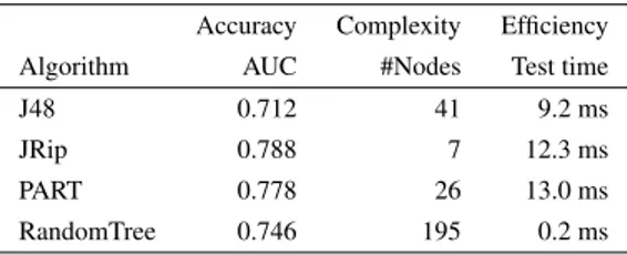
The group then discusses which metrics to use for attribute evaluation. A consen-sus decision is reached regarding the metrics to use for the accuracy and efficiency attributes: AUC and classification time, respectively. The motivation for using AUC is that it captures the relevant characteristics of classification performance irrespec-tive of class distribution and misclassification cost while the motivation for using classification time is that the tool must be responsive both when performing individ-ual classifications and batch processing of multiple software applications. It is more difficult to identify a suitable complexity metric. The machine learning researcher recommends a complexity metric (Gaines, 1996) that can be used measure the size of both rule-based and decision tree-based models (Allahyari and Lavesson, 2011). The group agrees to include the presented complexity metric and to restrict the choice of algorithms to rule and tree inducers since both algorithm types produce transparent models. The group decides to choose an acceptable range of [0.70, 0.90] for AUC based on a priori knowledge of reasonable classification performance on data sets with similar complexity. For the classification time metric, the group agrees that a range of [10, 50] in milli seconds elapsed per instance is reasonable. Finally, for the complexity metric and by taking into account the definition of the metric and the complexity of the classification problem, an acceptable range of [15, 30] is chosen. After the discussion about the selection of metrics and acceptable ranges, each stake-holder has formed an opinion about the other stakestake-holders and can thus assign expert
influence weights: V = 0.75 0.10 0.15 0.50 0.40 0.10 0.40 0.30 0.30 .
Table 4 presents the measurements of the selected criteria. Accuracy is assessed by measuring the AUC on independent test sets. Complexity is assessed by counting the number of decision nodes in each tree and rule-based model. Efficiency is assessed by measuring the average time it takes for a model to classify one data instance. The
Table 4 Case Study 2 – Measurements
Accuracy Complexity Efficiency
Algorithm AUC #Nodes Test time
J48 0.712 41 9.2 ms
JRip 0.788 7 12.3 ms
PART 0.778 26 13.0 ms
RandomTree 0.746 195 0.2 ms
measurements from Table 4 are now normalized based on the proposed acceptable ranges for each metric. The normalized scores are presented in Table 5.
Table 5 Case Study 2 – Normalized Measurements
Accuracy Complexity Efficiency
Algorithm AUC #Nodes Test time
J48 0.904 0 1 ms
JRip 1 1 0.942 ms
PART 0.987 0.266 0.925 ms
RandomTree 0.947 0 1 ms
5.4 Validation and Decision Phase
In this phase the validation engine is used to reduce the matrix of individual-based attribute weights W into a vector of consensus attribute weights a = [0.6, 0.28, 0.12]. Next a vector of group-based metric scores is produced for each classification algorithm based on the proposed acceptable ranges (see Eq. 1):
gJ48 = [ 0.569, 0, 1 ]
gJRip = [ 1, 1, 0.927 ]
gPART = [ 0.942, 0, 0.906 ]
Eq. 2 is then applied in order to calculate the group-based evaluation scores supported by all the stakeholders:
CEF(J48, D) = 0
CEF(JRip, D) = 0.991
CEF(PART, D) = 0
CEF(RandomTree, D) = 0.
Evidently, JRip represents the only valid choice given the previously defined con-straints and the individual metric scores on the selected data set, D.
6 Validity Threats
This article presents a method, APPrOVE, for systematic evaluation and selection of learning algorithms when there are multiple stakeholders, multiple goal metrics, and the overall objective is to include the most suitable algorithm in a software product. The method is analysed and demonstrated through two case studies. Yin (2009) pro-vides a detailed account of the case study as a research method, its variants, and the potential validity threats. Our approach has been to conduct descriptive case studies of a limited set of selected cases that are representative for the studied problem. The motivation for using the case study as a research method is that it provides a way to explore actors (in our case, stakeholders involved in decision making) and their interactions. We regard this approach as a feasible first step in analysing the suitabil-ity and validsuitabil-ity of APPrOVE as a method for decision making in the context of the studied problem. Yin (2009) argues that construct validity is especially problematic in case studies. We try to address this threat by involving multiple sources of evi-dence (each case involves a different context, set of data, stakeholders, metrics, and so on). Yin (2009) also review external validity, which deals with whether results are generalizable beyond the immediate case. There are some criticisms toward the use of single-case explanatory studies for producing statistical generalization. However, while our future aim is to investigate statistical generalization of APPrOVE through experiments, we believe that APPrOVE is at least analytically generalizable to similar cases of the studied problem.
With further regard to external validity, there is arguably also a non-representative research context threat to this type of case study analysis of a proposed method. That is, the case explored is not representative of cases from the studied problem. To address this threat, we have defined our case studies based two well-known and typical decision making scenarios from the application area. For both case studies, the outlined problem, the stakeholders, and the conflicting goals are taken from the real-world. The data sets and the particular choices of algorithms and metrics, how-ever, were selected by the authors to delimit the scope and enable analysis in a con-trolled setting. Another overall validity threat, inherent subjectivity, is difficult to fully avoid for many case study designs. Again, we strived to avoid this threat by defining two case studies from different application domains. In addition, the authors worked in disjoint sets of two researchers per case study group when obtaining results and performing analysis of results for the case studies.
7 Conclusions and Future Work
Machine learning algorithms are increasingly employed to solve real-world prob-lems. There is much potential in the use of machine learning for many real-world problems but it is important to stress that there also are many challenges that need to be addressed. A common result of prediction model evaluations in software en-gineering, for example, is conclusion instability. That is, a conclusion regarding an algorithm comparison in one project (e.g., algorithm A performs better than B) is false in another project (e.g., algorithm B performs better than A). There are many possible reasons for conclusion instability and a growing number of tangible ideas for reducing conclusion instability. This article is focused on an important, and re-lated, challenge: the choice of predictor for a real-world problem usually depends on multiple goals (e.g., high accuracy, low complexity, and high interpretability). These, sometimes conflicting, goals may be weighted differently by the involved stakehold-ers. There are no existing frameworks or methods for predictor comparison and se-lection with multiple goals and multiple stakeholders.
For classification problems, the most commonly used quality criterion is accu-racy, which may be evaluated using the area under the ROC curve, success rate, or some other metric. However, the use of accuracy as the sole quality criterion does not exhaustively capture the requirements of very many real-world applications. The question is; how to identify, prioritise, and evaluate multiple (perhaps conflicting) criteria. Moreover, few studies on machine learning evaluation consider the role and input of stakeholders and domain experts. There is arguably a need for a systematic and application-oriented evaluation approach.
This paper presents an extended version of a method, referred to as APPrOVE, which involves four sequential steps: i) identification of quality attributes, ii) attribute prioritisation, iii) metric selection, and iv) validation and evaluation. Two case studies are conducted to demonstrate the use of APPrOVE to validate and evaluate a set of candidate algorithms for a particular application. The case studies feature two differ-ent application domains (bioinformatics and software security) and typical stakehold-ers for each domain. In each case study, the APPrOVE method is used by the stake-holders to perform systematic evaluation and validation of a chosen set of learning algorithms for a particular learning task. It is clear from the use cases that APPrOVE is simple to apply but still provides a cohesive and transparent decision-making pro-cess. As the APPrOVE intermediate and final results in each use case demonstrate, it is straight-forward to analyze the prioritized candidate list to understand the as-signed priority for each candidate. In terms of applicability, the proposed method for evaluation is expected to generalize well to other supervised learning applications. The method should be generalizable to other learning applications (e.g., unsupervised learning) and to similar decision scenarios in other areas. That is, APPrOVE could potentially be modified to solve other decision tasks than machine learning algorithm selection if the generic task still is to rank candidate choices based on multiple met-rics and multiple experts. However, this article is completely focused on supervised classification learning applications.
There are several interesting directions for future work: in APPrOVE, we pri-oritise the quality attributes before selecting evaluation metrics. However, it is quite
possible to reverse the order of these steps. One benefit of this change in procedure is that the analytic hierarchy process can be extended to prioritise the metrics associated with each quality attribute as well. APPrOVE also involves the use of a multi-criteria metric, which yields a single quantity result. By enforcing the use of a univariate multi-criteria metric, rather than a multivariate multi-criteria method, it is possible to replace the learning metric of some of the existing supervised learning algorithms to optimise their performance toward application requirements during classifier genera-tion. In order to investigate this approach, we are currently working on re-designing a set of selected learning algorithms to allow for replacement of their learning metrics. Finally, our longterm aim is to further evaluate the generalizability of APPrOVE by conducting case studies for similar decision scenarios in other domains and for other applications in the studied domain (e.g., unsupervised learning cases).
References
Alizadeh et al A (2000) Distinct types of diffuse large b-cell lymphoma identified by gene expression profiling. Nature 403:503–511
Allahyari H, Lavesson N (2011) User-oriented assessment of classification model understandability. In: 11th Scandinavian Conference on Artificial Intelligence, IOS Press
Alon et al U (1999) Broad patterns of gene expression revealed by clustering analysis of tumor and normal colon tissues probed by oligonucleotide arrays. PNAS USA 96:6745–6750
Bucila C, Caruana R, Niculescu-Mizil A (2006) Model compression. In: 12th ACM SIGKDD International Conference on Knowledge Discovery and Data Mining, ACM Press
Dinesh Singh ea (2002) Gene expression correlates of clinical prostate cancer behav-ior. Cancer Cell 1:203–209
Fodor J, Roubens M (1994) Fuzzy Preference Modelling and Multicriteria Decision Support. Kluwer, Dordrecht
Freitas A (1998) On objective measures of rule interestingness. In: Second European Symposium on Principles of Data Mining & Knowledge Discovery, Springer Gaines B (1996) Transforming rules and trees into comprehensible knowledge
struc-tures. In: et al UF (ed) Advances in Knowledge Discovery and Data Mining, MIT Press, Cambridge, Mass., pp 205–226
Japkowicz N, Shah M (2011) Evaluating Learning Algorithms – A Classification Perspective. Cambridge
Lavesson N, Davidsson P (2007) Evaluating learning algorithms and classifiers. In-telligent Information & Database Systems 1(1):37–52
Lavesson N, Davidsson P (2008) Generic methods for multi-criteria evaluation. In: Eighth SIAM International Conference on Data Mining, SIAM Press
Lavesson N, Davidsson P (2010) Approve: Application-oriented validation and eval-uation of supervised learners. In: The Fifth IEEE International Conference on In-telligent Systems, IS’2010, IEEE Press
Lavesson N, Boldt M, Davidsson P, Jacobsson A (2010) Learning to detect spyware using end user license agreements. Knowledge and Information Systems
Menzies T, Shepperd M (2012) Special issue on repeatable results in software engi-neering prediction. Empirical Software Engiengi-neering 17(1–2)
Nakhaeizadeh G, Schnabl A (1997) Development of multi-criteria metrics for evalu-ation of data mining algorithms. In: Third internevalu-ational conference on knowledge discovery and data mining, AAAI Press, pp 37–42
Nakhaeizadeh G, Schnabl A (1998) Towards the personalization of algorithms eval-uation in data mining. In: Fourth international conference on knowledge discovery and data mining, AAAI Press, pp 289–293
Provost F, Fawcett T, Kohavi R (1998) The case against accuracy estimation for com-paring induction algorithms. In: 15th International Conference on Machine Learn-ing, Morgan Kaufmann Publishers, San Francisco, CA, USA, pp 445–453 Roubens M, Vincke P (1985) Preference Modelling. Springer-Verlag, Berlin Saaty TL (1980) The Analytic Hierarchy Process: Planning, Priority Setting,
Re-source Allocation. McGraw-Hill
Tsiporkova E, Boeva V (2004) Nonparametric recursive aggregation process. Kyber-netika, J of the Czech Society for Cybernetics and Inf Sciences 40(1)
Tsiporkova E, Boeva V (2006) Multi-step ranking of alternatives in a multi-criteria and multi-expert decision making environment. Information Sciences 176(18) Tsiporkova E, Tourwe T, Boeva V (2010) A collaborative decision support platform
for product release definition. In: The Fifth International Conference on Internet and Web Applications and Services, ICIW 2010, IEEE Press
Vaidya OS, Kumar S (2004) Analytic hierarchy process: An overview of applications. European Journal of Operational Research 169(1):1–29
Wang RW, Strong DM (1996) Beyond accuracy: What data quality means to data consumers. Journal of Management Information Systems 12(4)
Wohlin C, Andrews AA (2003) Prioritizing and assessing software project success factors and project characteristics using subjective data. Empirical Software Engi-neering 8(3):285–308
8 Appendix
8.1 The Analytic Hierarchy Process
AHP is executed by performing pairwise comparisons of a selected set of objectives, organised hierarchically into main objectives and sub objectives on as many levels as deemed suitable for the problem at hand. To limit the scope of the paper, we regard each identified quality attribute as a main objective. For an arbitrary prioritisation task
Table 6 pairwise comparison ordinal scale
Value1 Meaning
1 Attribute k and q are of equal importance
3 Attribute k is weakly more important than q
5 Attribute k is strongly more important than q
7 Attribute k is very strongly more important than q
9 Attribute k is absolutely more important than q
A common configuration of the pairwise comparison ordinal scale used by the Analytic Hierarchy Process.
1The numbers 2, 4, 6, and 8 represent intermediate values.
with n identified main attributes, the first step of AHP is to generate a n × n matrix, O, with pairwise comparison values. The attributes are now organised alphabetically and used as column and row labels for O. Let i and j denote index variables and let ∀(i = j)oi j= 1. Using the ordinal scale provided in Table 6, and for each attribute, i,
that is considered to be at least of equal importance to another attribute, j, assign a suitable value, v, to oi j. Correspondingly, let oji= 1/v.
The second step of AHP is to calculate the overall importance of each attribute. This step is performed by creating a n × n attribute weight matrix, Q. The value of each entry, qi j, of this matrix is then calculated by dividing the corresponding
pair-wise comparison value, oi j, with the sum of pairwise comparison values in the
col-umn the entry appears in. The overall importance, or weight, of each attribute is then obtained by calculating the average of the values in each row. Thus, the sum of at-tribute weights is 1, which is a prerequisite for the employed multi-criteria evaluation method.
8.2 The Large Preference Relation
One of the most important tools in preference modelling is the concept of a prefer-ence structure (Fodor and Roubens, 1994; Roubens and Vincke, 1985), suitable for representing the results of a pairwise comparison of a set of alternatives by a decision maker. A preference structure on a set A is a triplet (P, I, J) of binary relations on A, where P models strict preference, I indifference and J incomparability. These three
relations are defined as follows:
aPb⇔ a is strictly preferred to b; aIb ⇔ a and b are indifferent; aJb ⇔ a and b cannot be compared.
It is possible to associate a single reflexive relation R to any preference structure (P, I, J) such that it completely characterises the structure. It is defined as R = P ∪ I, and is usually called the large preference relation. It is clear that P and I represent the asymmetric and symmetric parts of R.
Consider a finite set of alternatives A and a function g that associates a positive real value g(a) to every a in A. Then the strict preference relation P can be defined as follows:
aPb ⇔ g(a) > g(b) , ∀(a, b) ∈ A2.
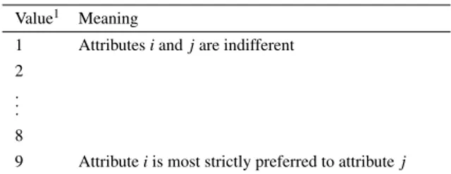
Let us consider an arbitrary prioritisation task with a set of n identified main at-tributes. The first step is to define a large preference relation over the set of attributes by constructing a n × n matrix, R, with pairwise comparison values. The above def-inition of strict preference relation implies that when attribute i is strictly preferred to attribute j then the corresponding pairwise comparison value ri j (interpreted as
the ratio g(i)/g( j)) must be greater than 1. Thus the matrix R can be generated by using the interval scale provided in Table 7. The next step is to calculate the overall importance (weight) wiof each attribute i:
wi= n
∑
j=1 ri j/n · n∑
k=1 rk j ! .It can easily be shown that the weight of each attribute i is, in fact, equal to g(i)/ ∑nj=1g( j)
(i.e., the attribute weights sum up to 1).
Table 7 pairwise comparison interval scale
Value1 Meaning
1 Attributes i and j are indifferent
2 . . . 8
9 Attribute i is most strictly preferred to attribute j
The pairwise comparison interval scale used by the Large Pref-erence Relation.
1The numbers 2, 3, 4, 5, 6, 7, 8 represent seven intermediate
values uniformly distributed between the indifference and most strict preference.