Prototype Extraction and Learning Using Prototypes in an Artificial Neural Network

Learning Using Prototypes in an

Artificial Neural Network

HS-IDA-MD-97-09

Fredrik Linåker

in an Artificial Neural Network

Fredrik Linåker

Submitted by Fredrik Linåker to the University of Skövde as a disserta-tion towards the degree of M.Sc. by examinadisserta-tion and dissertadisserta-tion in the Department of Computer Science.

October, 1997

I certify that all material in this dissertation which is not my own work has been identified and that no material is included for which a degree has already been conferred upon me.

Key words: Artificial Neural Networks, prototypes, learning, symbol grounding

A prototype is a general description which depicts what an entire set of exemplars, be-longing to a certain category, looks like. We investigate how prototypes, in the form of mathematical averages of a category’s exemplar vectors, can be represented, extracted, accessed, and used for learning in an Artificial Neural Network (ANN). From the method by which an ANN classifies exemplars into categories, we conclude that prototype access (the production of an extracted prototype) can be performed using a very simple architec-ture. We go on to show how the architecture can be used for prototype extraction by sim-ply exploiting how the back-propagation learning rule handles one-to-many mappings. We note that no extensions to the classification training sets are needed as long as they conform to certain restrictions. We then go on to show how the extracted prototypes can be used for the learning of new categories which are compositions of existing categories and we show how this can lead to reduced training sets and ultimately reduced learning times. A number of restrictions are noted which have to be considered in order for this to work. For example, the exemplar representations must be systematic and the categories linearly separable. The results, and other properties of our network, are compared with other architectures which also use some kind of prototype concept. Our conclusion is that prototype extraction and learning using prototypes is possible using a simple ANN archi-tecture. Finally, we relate our system to the symbol grounding problem and point out some directions for future work.

Contents

1 Introduction 1 1.1 Why prototypes ...1 1.2 Why ANNs ...2 1.2.1 Semantic networks...3 1.2.2 Frames ...3 1.2.3 ANNs ...4 1.3 Problem statement ...5 1.4 Overview ...6 2 Definitions 8 2.1 Exemplars ...8 2.2 Categories ...12 2.3 Prototypes ...17 3 Related work 19 3.1 The Coactivation Network ...19

3.1.1 Rationale ...19 3.1.2 Representation ...20 3.1.3 Architecture ...23 3.1.4 Process ...24 3.1.5 Problems ...29 3.1.6 Summary...31

3.2 Learning Vector Quantization ...31

3.2.1 Rationale ...32

3.2.2 Representation ...32

3.2.4 Process ...32 3.2.5 Problems ...33 3.2.6 Summary...34 4 REAC framework 35 4.1 Representation ...35 4.1.1 Exemplars ...36 4.1.2 Categories ...36 4.1.3 Prototypes ...38 4.2 Access...38 4.2.1 Classification ...38 4.2.2 Prototype access ...42 4.3 Extraction ...45

4.3.1 Back-propagation and one-to-many mappings...45

4.3.2 Resulting network architecture ...48

4.4 Composition ...49

4.4.1 The traditional approach ...50

4.4.2 The prototype approach ...52

5 Results 54 5.1 Implementation...54 5.2 Exemplar population ...55 5.3 Classifications ...56 5.3.1 Results ...56 5.3.2 Improving classifications...58 5.4 Extracted prototypes...59 5.4.1 Basic prototypes ...60

5.4.2 Higher level prototypes ...62

5.4.3 Prototype shifting ...63 5.5 Comparison ...66 5.5.1 Summary...70 5.6 Restrictions ...72 5.6.1 Identical prototypes ...72 5.6.2 Systematicity of Representation ...73

5.6.3 Linear separability ...74

5.6.4 Problems with composition ...77

6 Conclusions 80 6.1 The REAC aspects revisited...80

6.1.1 Representation ...80 6.1.2 Extraction...81 6.1.3 Access ...83 6.1.4 Composition...84 6.2 Symbol grounding ...86 6.2.1 Background...86 6.2.2 Relevance...87 6.2.3 Differences...88 6.3 Future work ...89 6.3.1 Iconic representations ...89 6.3.2 Combination methods...89 6.3.3 Other processes...90

6.3.4 Extending the network...91

6.3.5 Dynamical system...92

6.4 Final statement ...93

Acknowledgements 94

Chapter 1

Introduction

This thesis investigates how prototypes can be represented, extracted, accessed and used for composition in an Artificial Neural Network. A simple architecture is described which adheres to all these aspects and results from experiments using the architecture are pre-sented.

1.1 Why prototypes

A prototype can be considered a general description which depicts what the exemplars be-longing to a certain category look like. One way of creating such prototypes is to use a representation which depicts what a typical or average exemplar belonging to the catego-ry looks like. This is the approach taken in this thesis. The effects of having prototypes in a system have been used to help explain a wide range of issues (Lakoff, 1987):

cate-gories.

• Metonymic reasoning, which is the use of one or more objects as representatives for a larger group of objects.

• Gradient membership, the means by which individual exemplars may be more or less typical members of a category.

• Embodiment, connecting the representations used by the system with the real world in which it operates.

These are just some of the issues which are attributed to the existence of prototypes in a system. It is important to point out that while the above issues can be explained using pro-totypes, they do not depend on the existence of prototypes. That is, they may very well be explained without using any kind of prototypes. Such explanations are however outside the scope of this thesis, where we investigate how prototypes can be represented, extract-ed, accessextract-ed, and composed in an Artificial Neural Network (ANN).

1.2 Why ANNs

ANNs have a number of properties which make them appealing. For example, ANNs are able to extract information from a set of data. The most common use of this is to extract information which allows the network to recognize which exemplars belong to a certain category and which do not, i.e. to perform classifications.

ANNs allow for gradient membership in categories, e.g. different exemplars may produce different activation levels (i.e. different membership strengths) on a set of cate-gory units. Different degrees of confidence in the data may also be specified through the use of continuous activation values for the network’s input units.

achieved through the use of ANNs which directly operate on sensor inputs in autonomous agents such as robots (Dorffner, 1997).

Further, ANNs allow graceful degradation, default assignment and spontaneous generalization (Rumelhart et al., 1986). Some of these properties, e.g. default assign-ments, are also evident in alternative solutions such as semantic networks (Quillian, 1966) and frames (Minsky, 1975). But there are problems which these alternatives, as indicated in the following sections.

1.2.1 Semantic networks

Semantic networks represent information using nodes which are connected using ent labelled connections. There is no general interpretation of the nodes nor of the differ-ent type of links between them, which makes the networks susceptible to incorrect interpretation and use (Brachman, 1979). There are also other limitations on the represen-tations. For example, it is unclear how to define different degrees of certainty regarding information (Woods, 1975). This is a property which can be handled in ANNs using con-tinuous activation values to denote different degrees of certainty.

1.2.2 Frames

Frames represent information in packets where each packet deals with a specific situation. For example, a packet may contain information about birthday parties, i.e. that there are usually is cake, a number of guests, presents, and so on. The packets contain information about defaults, i.e. prototypical information, such as that the number of legs on a human being usually is two. This information can be overridden, were applicable. For example, a specific human being may be handicapped, only having one leg.

information is symbolic, i.e. there is no account for how the system is to be connected to the real world. For example, the system cannot recognize that it is at a birthday party—it has to be told so—and can only then make inferences about the situation it is in.

1.2.3 ANNs

Frames and semantic networks are implementations of symbol systems, i.e. they operate on a set of symbols which are interpreted by an outside observer (a human). The general properties which should be evident for any symbol system are defined by Fodor & Pyly-shyn (1988). Since all symbol systems should conform to these properties, any specific implementation of a symbol system should be able to translate into another—equal—sys-tem. More specifically, any symbol system, implemented using an architecture X, should be able to translate into a Turing machine (Turing, 1950) which functions identically to the original system. And consequently, if ANNs are mere implementations of symbol sys-tems, they can just as well be replaced by Turing Machines; so why use ANNs at all.

There are however claims that an ANN is not a mere implementation of a symbol system. It can operate on uninterpreted or sub-symbolic representations, for example sen-sorial inputs. ANNs have been put forward as a possible solution to the symbol grounding problem (Harnad, 1990), this is elaborated on further in section 6.2 where we discuss the possible relationship to our proposed prototype access, extraction and composition archi-tecture.

There exist at least two existing approaches, incorporating prototype or prototype concepts, which use ANN techniques. One of these is Learning Vector Quantization, which uses prototypes for classifications, and the other is the Coactivation Network which uses prototypes as category representations. These approaches are described in detail in chapter 3 and they later provide a reference point for our results.

1.3 Problem statement

An ANN is able to extract information from a set of exemplar vectors, which allows the network to recognize which exemplar vectors belong to a category and which do not. We intend to investigate if it is also able to extract information about what typical exemplars (prototypes) for each category looks like. We also intend to investigate whether proto-types can be used as representations for a larger group of exemplars (cf. metonymic rea-soning) when learning new categories. In our experiments, we compare our results with the categories extracted using Robins’ Coactivation Network (section 3.1) which is able to extract categories which are arranged in hierarchies. We will investigate whether the categories at the lowest hierarchical level can be extracted and then composed into more abstract categories (higher up in the hierarchy) using an ANN. Robins’ experiments pro-vide a reference point for our results.

We intend to investigate this through a process which should give answers to four different aspects, which we call the REAC aspects (Representation, Extraction, Access and Composition), all relating to having prototypes in an ANN. Each of these aspects de-pend on that the previous aspects have been resolved, e.g. Access can only be done on pro-totypes if we first have defined (and implemented) Extraction of the propro-totypes.

1. Representation. How can prototypes be represented in an ANN, i.e. on what

net-work unit(s) should the prototypes be represented and what should each unit encode, what limitations exist for the representations and what kind of systematic-ity is required.

2. Extraction. Can an ANN extract prototypes from training sets consisting of

exem-plar vectors and their corresponding classification, what methods can be used for extraction and how can the extracted information be stored in the network.

3. Access. Can the prototype representation be accessed for a given category, i.e. can

the network produce the prototype representation if all we supply is which of the categories we are interested in and what are the architectural implications of hav-ing accessible prototypes.

4. Composition. Given that the system has extracted the prototypes for a set of

cate-gories, can the network then extract new category prototypes, for new catecate-gories, using only the existing prototypes, i.e. without using any further exemplars.

Our intent is to answer the above questions by designing an ANN architecture. During the creation of the architecture, we will investigate how the REAC aspects influence our de-sign choices and we will note important implications for processing and representation in the ANN.

1.4 Overview

In chapter 2 we define the terminology used throughout the thesis. There are three main concepts, namely exemplars, categories and prototypes; these concepts are described and examples of each are given.

Chapter 3 describes some of the related work on having prototypes in an ANN. The main thrust of this chapter is A. V. Robins’ Coactivation Network which is able to extract and access generalized representations (similar to prototypes), using unsupervised learn-ing.

In chapter 4, we describe the framework of an architecture which fulfils the REAC aspects. We describe how the back-propagation algorithm handles one-to-many mappings and how this can be explored for prototype extraction and we describe how the network can learn new categories using the existent category prototypes.

Chapter 5 lists some of the results which were obtained using the network described in chapter 4 to extract and compose category prototypes.

Finally, in chapter 6, we discuss the results, we relate our approach to Harnad’s symbol grounding problem, and we give some indications for future work.

Chapter 2

Definitions

This chapter describes the three basic concepts used throughout this thesis, namely exem-plars, categories and prototypes. Exemplars are denoted using italicized lower-case letters and an accompanying number (indicating it is just one of many similar exemplars), e.g.

fish1, fish2 and fish3. Category names are also italicized, but start using an capital letter

and have no accompanying number, e.g. Fish, Cat and Dog. Prototypes are denoted using the name of the category which it is coupled to together with the word “prototype”, e.g. the Fish prototype and the Dog prototype.

2.1 Exemplars

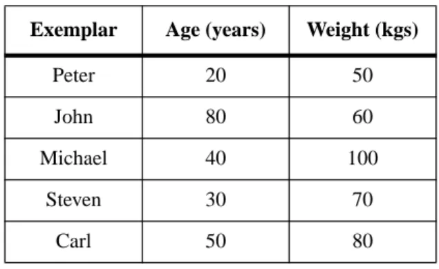
Exemplars may be actual real-world entities or completely abstract concepts; as long as a representation can be created for the object it is an eligible exemplar. For example, a cat may be represented by a vector of values indicating its height, weight, age etc. as depicted

in Figure 1.

Figure 1: An exemplar and its representation

Different cats get different representations. There must however exist a degree of systematicity in these representations, namely that similar exemplars should in some

sense have similar representation1. Generalization, i.e. the ability to infer new informa-tion from existing knowledge, is based on this systematicity of representainforma-tion; similar ex-emplars with similar representations are treated in the same manner. This enables the system to handle new, not previously encountered, exemplars in a manner which is con-sistent with the knowledge of previously presented exemplars, as described in section 2.2. Also, without this systematicity of representation, meaningful prototypes cannot be ex-tracted, as shown in section 2.3.

Further, the representations should be distributed2 in order to allow expression of different degrees of similarity:

In localist representations, all of the vectors representing items are, by defini-tion, perpendicular to one another and equidistant (Hamming or Euclidian dis-tance). Thus it is difficult to capture similarities and differences in localist representation space (although it can be done by explicit marking). (Sharkey, 1991, pp. 148 - 149)

1. And conversely, dissimilar exemplars should have dissimilar representation. This precludes the mapping where all exemplars are represented using the same representation, which also would be quite pointless in that we could not classify the exemplars into different categories.

2. The representation should be a pattern of activation distributed over several units and these units should participate in the representation of several exemplars, i.e. it should not consist of activat-ing of a sactivat-ingle unit representactivat-ing the particular exemplar.

Exemplars are represented using a vector consisting of one or more values1, whose elements can be said to indicate a point in hyperspace for the exemplar. For example, con-sider the population consisting of five patient exemplars shown in Table 1.

Table 1: A sample population consisting of five exemplars represented using a vector with two elements each (age and weight)

The exemplars can be displayed in a two-dimensional space where each vector ele-ment indicates the position in one of the dimensions, as shown in Figure 2. The interval for each dimension is determined by the set of possible, or likely, values.

In this case, the Weight dimension may range between 0 to several hundred kilo-grams, depending on the patient characteristics. Likewise, the Age dimension ranges from 0 to 120, or so, years. In both cases it is hard to create a closed interval, trading scope for detail, which adequately can handle all exemplars we may want to represent in the future.

1. This makes it very hard, in some cases, to create representations for a concept, when it is not possible to measure its characteristics, i.e. to quantify it.

Exemplar Age (years) Weight (kgs)

Peter 20 50

John 80 60

Michael 40 100

Steven 30 70

Figure 2: Five points representing five different patients using their age and weight characteristics

When working with ANNs, the activation on a unit usually represents the location in one of the dimensions. By using several units, each one representing one of the dimen-sions, we get a pattern of activation which indicates a position in hyperspace.

There are limitations on the range of activation for a network unit; here each unit can only take on a value between 0.0 and 1.0 (when the activation takes on values around 0.0, the unit is said to be inactive, and similarly, values around 1.0 indicate that the unit is active). We can thereby draw the representational space as a bounded area, as depicted in Figure 3; the bounding values should be interpreted as 0.0 and 1.0, respectively.

The interpretation, or “meaning” of each unit does not have to be defined as long as we do not want to encode any actual (real-world) exemplars, but rather can do with a gen-erated set of representations, as described in section 3.1.2. The labels on the axes can thus be omitted, as depicted in Figure 3.

Peter Age Weight 20 40 60 80 0 0 20 40 60 80 100 Michael John Steven Carl

Figure 3: Representational space for nine exemplars using a two-dimensional, bound-ed, distributed representation where similar exemplars have similar represen-tation

In summary, an exemplar is any object (idea/concept/entity) for which we can cre-ate a distributed representation where similar objects end up with similar representation.

2.2 Categories

The exemplars can be classified as belonging to one or more categories. The approach for representing these categories is to divide the representational space using some kind of boundary lines. This is just one of many proposed ideas for representing categories. For example, a category may be defined by enumerating all exemplars belonging to it, or it may be defined using a set of rules which determine the necessary and sufficient features for category membership (Lakoff, 1987). Yet another way of defining categories is to use a set of prototypes which determine category membership (Reed, 1972).

An exemplar is represented using a point in hyperspace, the position of this point in relation to these boundary lines determine which categories (if any) the exemplar belongs to. For example, the nine exemplars in Figure 3 may be divided into the three categories

dog1 dog2 dog3 fish1 fish2 fish3 cat1 cat2 cat3

Cat, Dog, and Fish as depicted in Figure 4.

Figure 4: The nine exemplars classified into three categories, the boundaries of these categories divide the representational space into three smaller areas

The systematicity of having similar representation for similar exemplars allows for generalization to new exemplars. For example, if we were to confront the system with a previously unseen exemplar, fish4, the system would correctly classify it as a Fish (see Figure 5), given that its representation is sufficiently similar to that of the other fish ex-emplars. dog1 dog2 dog3 fish1 fish2 fish3 cat1 cat2 cat3 Cat Dog Fish

Figure 5: Generalization occurs when a new fish exemplar is introduced; it is correctly treated as a fish since it resembles the previous fish exemplars, i.e. it falls in the Fish area

Categories can be combined to form more abstract, categories. For example, the Cat and Dog categories can be combined into the larger category Mammal, as shown in Figure 6.

Figure 6: The two categories Dog and Cat can be combined to form a more general cat-egory Mammal which contains six exemplars

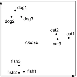
An even more abstract category Animal can be formed by combining the Mammal

Cat Dog Fish new exemplar dog1 dog2 dog3 fish1 fish2 fish3 cat1 cat2 cat3 Mammal Fish

and Fish category, as shown in Figure 7.

Figure 7: A category Animal can be formed by combining all categories into one very general category which contains all nine exemplars

The composition of categories into more abstract categories is an important con-struct in knowledge representation research, where they can be used to create type hierar-chies, which are hierarchical arrangements of categories into inheritance trees, as shown in Figure 8 (Robins, 1989b, p. 346).

Figure 8: An inheritance tree for the categories Dog, Cat, Fish, Mammal and Animal

The more general a category is, the more inclusive it is. For example, the category

Dog contains 3 exemplars, Mammal contains 6, and the even more abstract category

An-dog1 dog2 dog3 fish1 fish2 fish3 cat1 cat2 cat3 Animal Animal Mammal Fish Dog Cat

imal contains 9 exemplars.

An exemplar can thus belong to several categories, at different abstraction levels, at once. For example, the dog1 exemplar belongs to Dog, Mammal and Animal categories. On some occasions an exemplar could belong to several categories at the same level, as shown in Figure 9. This is more commonly called multiple inheritance.

Figure 9: A multiple inheritance graph where a Student employee is both an Employee and a Student

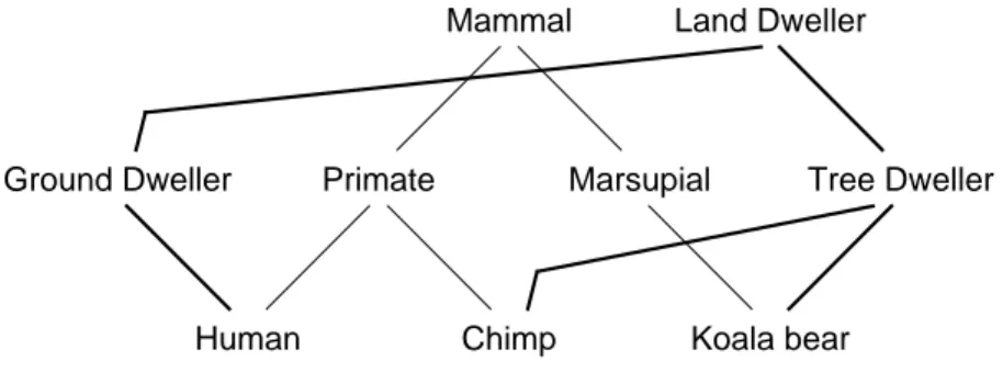
Further, an exemplar may be classified on different dimensions. For example, an an-imal exemplar may be classified on the basis of the physical taxonomy of the entities, and on their characteristic habitat, as shown in Figure 10. (Robins, 1989a, section 5.6)

Figure 10: An example where there are multiple dimensions (Robins, 1989a, p. 174)

As Robins (1989a, p. 174) points out, if the system should handle more than a single Person

Employee

Student employee Student

Primate Marsupial

Human Chimp Koala bear

Land Dweller

Ground Dweller Tree Dweller

dimension of information, i.e. if it should handle tangled hierarchies, the inheritance tree needs to be replaced with a directed acyclic inheritance graph (see e.g. Touretzky, 1986), which look similar to the graph in Figure 10. This is also the case if the system is to handle multiple inheritance.

2.3 Prototypes

Each category groups together one or more exemplars. These exemplars all have individ-ual properties, some of which may not be shared by any other exemplar in the same cate-gory. A prototype is an abstraction of the category’s exemplar properties, indicating what a typical exemplar belonging to the category looks like.

As indicated by Reed (1972), one way of calculating the prototype for a category is to take the mean (average) of each value in the exemplar vector for every exemplar be-longing to the category. This places the prototypes in the middle of each category’s cluster of exemplars, as depicted in Figure 11. This is just one possible way of viewing a proto-type. For example, an actual exemplar, which is considered “typical” in some sense, may be selected as the prototype, or even a whole set of typical exemplars may together con-stitute some kind of prototype concept.

Figure 11: Prototypes for the three categories Dog, Cat and Fish

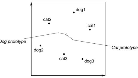
If the exemplar representations were not created using similar representations for similar exemplars, the prototype could end up being the same as the prototype for some other category, as depicted in Figure 12.

Figure 12: Prototypes (which are identical) for the two categories Dog and Cat, where

similar exemplars are not represented by similar vectors dog1 dog2 dog3 fish1 fish2 fish3 cat1 cat2 cat3 Dog prototype Cat prototype Fish prototype dog1 dog2 dog3 cat1 cat2 cat3 Dog prototype Cat prototype

Chapter 3

Related work

Two existing ANN classification systems are described in this chapter. They both use concepts corresponding to prototypes.

3.1 The Coactivation Network

Anthony Robins (1989a, 1989b, 1992) describes an architecture which can extract regu-larities in coactivation from a set of vectors, each one representing a perceived item, and use these regularities to access more general representations for the perceived items. The perceived items correspond to exemplars, and the “more general representations” roughly correspond to categories and prototypes (each category is represented using its prototype).

3.1.1 Rationale

config-urations of active units are most common. More specifically, it is the coactivation which is important, i.e. which units are frequently active simultaneously.

When the system then is presented with a vector, it calculates to which degree this specific configurations has appeared in the vector population. If there are units which are now active, which typically are not active, the unit is turned off, making the representation “more typical”, or “general”, in some sense. Similarly, if there is some unit which is not active in the present representation, but which typically should be active, the unit is turned on, again making the representation more general. Basically, this process makes the spe-cific representation more consistent with the information available about the entire popu-lation.

For example, if the vector population contains information about many different birds, the system may calculate that the probability of a bird being able to fly, let us call it the bird’s “fly-ability”, is close to 1.0. If the system then is presented with a specific bird vector, e.g. for a penguin, which cannot fly (fly-ability = 0.0), the system gradually mod-ifies the representation as to changing the fly-ability from 0.0 to 1.0. We end up with a representation which in some sense is a more general instance of a penguin, indicating that the vector belongs to a more abstract category (bird), which typically is able to fly.

3.1.2 Representation

The Coactivation Network is based on that similar perceived items get similar represen-tations. This means that there are clusters of vectors, encoding similar perceived items, which create similar patterns of activation on the network units. The network is then able to partition the units into groups, corresponding to these patterns, using unsupervised learning. (Robins, 1989a, p. 74)

A perceived item is encoded using a vector of values, where each vector element indicates to what degree a specific feature is applicable to the perceived item. This is called having specified semantics1.

Since Robins did not encode any actual perceived items, there was no need to define exactly what each vector element (i.e. unit in the Coactivation Network) is supposed to encode:

As noted by Hinton (1981, p. 177), however, it is possible to assume that units have a semantic interpretation, and construct perceived items in accordance with the general constraints of specified semantics, without actually giving an interpretation for each unit. This is the method used in constructing popula-tions for the various implementapopula-tions described in this thesis. (Robins, 1989a, p. 27, original emphasis)

This allowed the vector population to be generated using a set of templates. A number of vectors were generated from each template by applying random modifications to some of the template’s values. Provided that the modifications did not distort the tem-plates too much, the generated population now consists of vectors which can be grouped into categories since there exist clusters of similar vectors; namely of those vectors which originate from the same template.

In fact, what Robins’ coactivation technique tries to do is to extract these templates from the resulting vector population, i.e. it tries to eliminate the “individual-specific noise” and create generalized representations/prototypes for clusters of similar vectors.

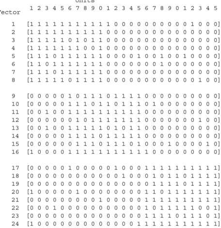
The vector population used by Robins was generated from the three binary vector templates shown in Figure 13.

1. This differs from unspecified semantics where items may be represented using arbitrarily cre-ated vectors, not providing the system with the means of detecting regularities in coactivation since there may be none.

Figure 13: Templates used for generating the vector population

Each template was used to generate eight individual vectors by swapping the tem-plate bits at a 10 % probability, ending up with the 24 vectors depicted in Figure 14.

Figure 14: Vector population generated from the three templates with bits swapped at a

10 % probability (Population H, Robins, 1989a, p. 128)

Calculating the Hamming closeness for the population of vectors, it is evident that vectors 1 - 8, 9- 16 and 17 - 24 form clusters of high similarity; vectors 1 - 16 also form a

1 2 3 4 5 6 7 8 9 0 1 2 3 4 5 6 7 8 9 0 1 2 3 4 5 [1 1 1 1 1 1 1 1 1 1 0 0 0 0 0 0 0 0 0 0 0 0 0 0 0] [0 0 0 0 0 1 1 1 1 1 1 1 1 1 1 0 0 0 0 0 0 0 0 0 0] [0 0 0 0 0 0 0 0 0 0 0 0 0 0 0 1 1 1 1 1 1 1 1 1 1] 1 2 3 Template Units 1 2 3 4 5 6 7 8 9 0 1 2 3 4 5 6 7 8 9 0 1 2 3 4 5 [1 1 1 1 1 1 1 1 1 1 1 0 0 0 0 0 0 0 0 0 0 1 0 0 0] [1 1 1 1 1 1 1 1 1 1 0 0 0 0 0 0 0 0 0 0 0 0 0 0 0] [1 1 1 1 1 0 1 0 1 1 0 0 0 0 0 0 0 0 0 0 0 0 0 0 0] [1 1 1 1 1 1 1 0 0 1 0 0 0 0 0 0 0 0 0 0 0 0 0 0 0] [1 1 1 0 1 1 1 1 1 1 0 0 0 0 1 0 0 1 0 0 1 0 0 0 0] [1 1 0 1 1 1 1 1 1 1 0 0 0 0 0 0 0 1 0 0 0 0 0 0 0] [1 1 1 0 1 1 1 1 1 1 0 0 0 0 0 0 0 0 0 0 0 0 0 0 0] [1 1 1 1 1 0 1 1 1 1 0 0 0 0 0 0 0 0 0 0 0 0 1 0 0] [0 0 0 0 0 1 0 1 1 1 0 1 1 1 1 0 0 0 0 0 0 0 0 0 0] [0 0 0 0 0 1 1 1 0 1 1 0 1 1 1 0 1 0 0 0 0 0 0 0 0] [0 0 1 0 0 1 1 1 1 1 1 1 1 1 1 0 0 0 0 0 0 0 0 0 0] [0 0 0 0 0 0 1 0 1 1 1 1 1 1 1 0 0 0 0 0 0 0 1 0 0] [0 0 1 0 0 1 1 1 1 1 0 1 0 1 1 0 0 0 0 0 0 0 0 0 0] [0 0 0 0 0 1 1 1 1 0 1 1 1 1 1 0 0 0 0 0 0 0 0 0 0] [0 0 0 0 0 0 1 1 1 0 1 1 1 0 1 0 0 0 1 0 0 0 0 1 0] [1 0 0 0 0 1 1 1 1 1 1 1 1 1 1 1 0 0 0 0 0 0 0 0 0] [0 0 0 0 0 1 0 0 0 0 0 1 0 0 0 1 1 1 1 1 1 1 1 1 1] [0 0 0 0 0 0 0 0 0 0 0 0 1 0 0 0 1 0 1 1 0 1 1 1 1] [0 0 0 0 0 0 0 0 0 0 0 0 0 0 0 0 1 1 1 1 0 1 1 1 1] [1 0 0 0 0 0 1 0 0 0 0 0 0 0 0 1 1 0 1 1 1 1 1 1 1] [0 0 0 0 0 0 0 0 0 1 0 0 0 0 0 1 1 1 1 1 1 1 1 1 1] [0 0 0 1 0 0 0 0 0 0 0 0 0 0 0 1 0 1 1 1 1 1 0 0 1] [0 0 0 0 0 0 0 0 0 0 0 0 0 0 0 1 1 1 1 0 1 1 1 0 1] [1 0 0 0 0 0 0 0 0 0 0 0 0 0 1 1 1 1 1 1 1 1 1 1 1] 1 2 3 4 5 6 7 8 9 10 11 12 13 14 15 16 17 18 19 20 21 22 23 24 Vector Units

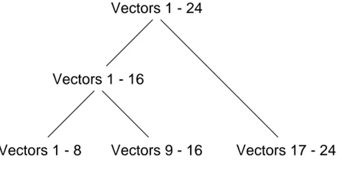
cluster but with slightly lower similarity (Robins, 1989a, p. 76). The vector population clusterings can be described using the hierarchy outlined in Figure 15.

Figure 15: Hierarchical organisation of the major clusterings in the vector population

The hierarchy depicts the structure of the vector population; this structure is used further on as a reference point with which the resulting classification is compared.

3.1.3 Architecture

The vector length determines the number of units in the Coactivation Network. Using the population of 25-bit vectors presented in Figure 14, the coactivation consists of 25 asym-metrically connected units. The coactivation weight on the connection from a unit x to unit

y is calculated using the formula in Equation 1. (Equation 4.1, Robins, 1989a, p. 93)

(1)

Considering the vector population in Figure 14, the connection from unit 1 to unit 9 is set to 8 / 11 (approximately 0.73) since unit 1 is active in eleven vectors, and unit 1 is coactive with unit 9 in eight of the vectors. The connection from unit 9 to unit 1, on the other hand, is set to 8 / 14 (approximately 0.57) since unit 9 is active in fourteen vectors

Vectors 1 - 24

Vectors 1 - 16

Vectors 17 - 24 Vectors 1 - 8 Vectors 9 - 16

weight_xy

∑

(activation x( ) activation y⋅ ( )) activation x( )

( )

∑

---=

but it is only coactive with unit 1 in eight vectors. This means that if we know that unit 1 is active, it is quite acceptable to assume that unit 9 is also active, or “coactive”, from what we know about the vector population. On the other hand, if we know that unit 9 is active, it is not so clear-cut whether unit 1 is active or not based on the coactivation information we have about the population.

The coactivation weights are calculated once, using the entire vector population, and the weights are not updated further during classification. Because the weights are not learned, but rather pre-calculated using the entire population, there is no apparent manner in which to introduce new vectors into the population without requiring access to the other vectors in order to get the new coactivation weight values.

The architecture thus consist of a set of units, asymmetrically connected to each oth-er, with static weights set according to the coactivation frequency, calculated using the en-tire vector population. Each of the interconnected units has two activation states which are iteratively updated by the processes described in the next section.

3.1.4 Process

When the network is presented with the vector for a perceived item, after a number of steps, the network settles on a new vector which is a more general representation of the original vector. The active units in this new vector form the “domain” for the perceived item, and this new vector is “more consistent” (than the original vector) with the coacti-vation information calculated from the entire vector population. Essentially, the network produces an answer to the following question, where X denotes the perceived item:

- What does a more typical X look like?

1. Presenting the input pattern. The vector for the perceived item is presented to the

network by setting the activation level of each unit accordingly.

2. Setting the centrality criterion. The centrality criterion is a value (in the range 0

to 1) which specifies the “level” of the target domain, i.e. it specifies to what extent units should be included in the domain. The lower the centrality criterion, the more units are included in the domain which in turn means that we get a more general domain1. (The most general category is that whose domain includes all units.) 3. Calculating the centrality distribution. The centrality value of each unit is

calcu-lated by taking the average of the incoming coactivation which is calcucalcu-lated by multiplying the coactivation weight of each incoming connection with the activa-tion value of the unit from which it emanates. Each unit thus has two values: the activation level, which is the “normal” value used in ANNs, and the centrality value which denotes to which extent the unit is typically coactive with the current configuration of active units. The combined pattern of all units’ centrality values is called the centrality distribution and it constitutes a kind of “prototype” representa-tion for the category (Robins, 1992, p. 48).

4. Correcting the largest violation. Each unit’s centrality value is compared with the

centrality criterion. If the unit’s activation level indicates that the unit is “on” and the centrality value is below the centrality criterion, i.e. it indicates that it should be “off”, then there exists a (negative) violation. Similarly, if the activation level says “off” but the centrality value is above the centrality criterion there exists a (posi-tive) violation. The absolute violation for each unit is calculated; if there are no violations at all the process ends here. If a violation exists, the unit with the largest

1. This is in contrast to “the subvector approach” where more general types are described by fewer and fewer units, namely those units which are invariant for all members (Rumelhart et al., 1986, p. 84). Robins notes that there are some inherent problems with that approach, specifically the subvector definition of type representations which is circular (Robins, 1989a, section 3.3).

absolute violation is chosen and its activation level is switched “on” (in the case of a positive violation) or “off” (in the case of a negative violation). We now have a new pattern of activation which in turn produces a new centrality distribution, i.e. the process continues on step 2 and onward until there no longer exists any viola-tion.

The stable pattern of activation which we finally arrive at is considered to be the domain of the original input. For example, domain access using vector 5 from the vector popula-tion in Figure 14, using a centrality criterion of 0.45, generates the following (Robins, 1989a, p. 130) initial state:

unit 1 activation 1 centrality 0.61 unit 2 activation 1 centrality 0.5 unit 3 activation 1 centrality 0.52 unit 4 activation 0 centrality 0.4 unit 5 activation 1 centrality 0.5 unit 6 activation 1 centrality 0.66 unit 7 activation 1 centrality 0.8 unit 8 activation 1 centrality 0.66 unit 9 activation 1 centrality 0.71 unit 10 activation 1 centrality 0.78 unit 11 activation 0 centrality 0.27 unit 12 activation 0 centrality 0.28 unit 13 activation 0 centrality 0.24 unit 14 activation 0 centrality 0.26 unit 15 activation 1 centrality 0.37 unit 16 activation 0 centrality 0.21 unit 17 activation 0 centrality 0.18 unit 18 activation 1 centrality 0.25 unit 19 activation 0 centrality 0.2 unit 20 activation 0 centrality 0.15 unit 21 activation 1 centrality 0.19 unit 22 activation 0 centrality 0.24 unit 23 activation 0 centrality 0.24 unit 24 activation 0 centrality 0.16 unit 25 activation 0 centrality 0.17

The largest violation is found on unit 21 (activation = 1 but centrality < centrality criterion); it is a negative violation of size 0.26 (centrality 0.19 centrality criterion 0.45 = -0.26). Consequently, this unit is turned “off” by setting its activation level to zero and we get the following state:

unit 2 activation 1 centrality 0.53 unit 3 activation 1 centrality 0.56 unit 4 activation 0 centrality 0.42 unit 5 activation 1 centrality 0.53 unit 6 activation 1 centrality 0.7 unit 7 activation 1 centrality 0.85 unit 8 activation 1 centrality 0.72 unit 9 activation 1 centrality 0.77 unit 10 activation 1 centrality 0.83 unit 11 activation 0 centrality 0.3 unit 12 activation 0 centrality 0.3 unit 13 activation 0 centrality 0.26 unit 14 activation 0 centrality 0.29 unit 15 activation 1 centrality 0.38 unit 16 activation 0 centrality 0.15 unit 17 activation 0 centrality 0.14 unit 18 activation 1 centrality 0.19 unit 19 activation 0 centrality 0.14 unit 20 activation 0 centrality 0.1 unit 21 activation 0 centrality 0.19 unit 22 activation 0 centrality 0.19 unit 23 activation 0 centrality 0.19 unit 24 activation 0 centrality 0.12 unit 25 activation 0 centrality 0.11

This time the largest violation is found on unit 18, again a negative violation of size 0.26. This unit is consequently turned “off”, and the process continues. After a couple of itera-tions, turning off unit 15 and turning on unit 4, we no longer have any violations and the following state:

unit 1 activation 1 centrality 0.72 unit 2 activation 1 centrality 0.65 unit 3 activation 1 centrality 0.66 unit 4 activation 1 centrality 0.48 unit 5 activation 1 centrality 0.65 unit 6 activation 1 centrality 0.72 unit 7 activation 1 centrality 0.93 unit 8 activation 1 centrality 0.74 unit 9 activation 1 centrality 0.82 unit 10 activation 1 centrality 0.89 unit 11 activation 0 centrality 0.28 unit 12 activation 0 centrality 0.24 unit 13 activation 0 centrality 0.22 unit 14 activation 0 centrality 0.24 unit 15 activation 0 centrality 0.35 unit 16 activation 0 centrality 0.1 unit 17 activation 0 centrality 0.07 unit 18 activation 0 centrality 0.2 unit 19 activation 0 centrality 0.07 unit 20 activation 0 centrality 0.05 unit 21 activation 0 centrality 0.13 unit 22 activation 0 centrality 0.15 unit 23 activation 0 centrality 0.15 unit 24 activation 0 centrality 0.06 unit 25 activation 0 centrality 0.05

This final state identifies units 1 - 10 as the domain of vector 5. Presenting the vectors 1 through 8 with the same centrality criterion all converge on this state. Vectors 9 - 16 all generate a state which has units 6 - 15 as its domain, and the domain of vectors 17 - 24 includes units 16 - 25. That is, the network has successfully clustered the vectors into the three basic level groupings which exist in the population, according with the clustering shown in Figure 15.

Using the vector generated by processing any of the vectors 1 - 16 (at a centrality criterion of 0.45), and lowering the centrality criterion to 0.25, we end up with the follow-ing state:

unit 1 activation 1 centrality 0.53 unit 2 activation 1 centrality 0.43 unit 3 activation 1 centrality 0.51 unit 4 activation 1 centrality 0.32 unit 5 activation 1 centrality 0.43 unit 6 activation 1 centrality 0.72 unit 7 activation 1 centrality 0.89 unit 8 activation 1 centrality 0.76 unit 9 activation 1 centrality 0.82 unit 10 activation 1 centrality 0.83 unit 11 activation 1 centrality 0.4 unit 12 activation 1 centrality 0.39 unit 13 activation 1 centrality 0.38 unit 14 activation 1 centrality 0.38 unit 15 activation 1 centrality 0.51 unit 16 activation 0 centrality 0.12 unit 17 activation 0 centrality 0.1 unit 18 activation 0 centrality 0.16 unit 19 activation 0 centrality 0.11 unit 20 activation 0 centrality 0.06 unit 21 activation 0 centrality 0.11 unit 22 activation 0 centrality 0.13 unit 23 activation 0 centrality 0.16 unit 24 activation 0 centrality 0.1 unit 25 activation 0 centrality 0.06

The domain of vectors 1 - 16 thus is the units 1 - 15, whereas presenting the vector gen-erated by vectors 17 - 24 (at a centrality criterion of 0.45), and lowering the centrality to 0.25, we get the domain of units 16 - 25. This means that the network also has learned to cluster the vectors into the two middle level groupings depicted in Figure 15.

Similarly, using a vector generated by using the centrality criterion of 0.25, and now lowering it to 0.1, we get a vector whose domain is units 1 - 25, i.e. the network clusters all vectors into the same category. The domains of all these clusterings can be depicted as in Figure 16.

Figure 16: Hierarchical organisation of the network’s clustering

If we compare the network’s clustering to the “reference structure” in Figure 15, we see that it has successfully extracted the main clusterings which exist in the population.

3.1.5 Problems

As Robins acknowledges, there is the problem of finding a suitable centrality criterion, the choice of which is very important in that it controls what units are included in the do-main. There is no apparent way to find “good” centrality criteria:

We cannot yet suggest in detail what sort of process would set the criterion in a self-contained PDP system. We suggest that the accessing of type informa-tion in general must involve a specificainforma-tion of the “level” in the hierarchy which is intended, even if this is a default value in most cases. (If asked “what sort of thing is a dog”, one is likely to reply “an animal” a default response -unless pressed for more or less generality.) We suggest, therefore, that in a self contained PDP system, the mechanism which initiates the access of type infor-mation will necessarily specify a (possibly default) criterion / level. (Robins, 1989a, p. 129, footnote)

Further, there is the problem of finding the largest violation. This involves a global Units 1 - 25

Units 1 - 15

Units 16 - 25 Units 1 - 10 Units 6 - 15

operation, namely the comparison of each violation size with every other which is not in accordance with the PDP principle of only using information which is available locally at each unit / connection. Robins does suggest a possible escape route from this global op-eration:

In these initial implementations of domain access the ordering strategy and the adjustment of unit states are simple and deterministic mechanisms. We regard this as an approximation to a more interesting approach (which we hope to ex-plore in future research) based on a probabilistic strategy of adjustment, name-ly, that units in violation of the criterion would have (in any given time period / cycle) a probability of adjusting their states which is directly proportional to the magnitude of their violation. (Robins, 1989a, p. 130, footnote)

The described processes can only access information arranged in inheritance trees, i.e. it cannot handle categories arranged in directed acyclic graphs. Inheritance trees are handled using the centrality criterion. It provides the necessary context to create the one-to-one mapping (between a perceived item input and a general representation output). The centrality criterion specifies at what level in the tree the resulting general representation should lay, lower centrality tends to generate more abstract representations. The system can only indicate one—and only one—category as an answer. A perceived item, com-bined with a given centrality criterion, can thus belong to one and only one category which in essence makes it impossible to have multiple inheritance hierarchies; even if the dimensions of information is represented on separate patterns of units. Some kind of con-text must help the system select in which dimension we want the answer to lay:

In other words, in order to represent multiple hierarchies, the domains meth-ods described above must be constrained by superordinate mechanisms which select a group of units (the desired dimension of information) to participate in domain access. (Robins, 1989b, p. 359)

The categories are represented using a pattern of activation which necessarily is bi-nary. This is a severe limitation, especially when working with short length vectors; if the

perceived item is represented using only two continuous values, there can only be four dif-ferent categories.

Finally, there is no learning scheme by with the coactivation weights are set. Intro-ducing information about other perceived items is not a trivial operation; the network needs to access the entire vector population in order to get the new coactivation values.

3.1.6 Summary

The Coactivation Network is an architecture which can be used to generate more general representations of perceived items; a process which is guided by the extracted coactiva-tion informacoactiva-tion about the entire vector populacoactiva-tion.

The activation and the coactivation information is combined to form centrality dis-tributions which can be considered as “prototypes” of the categories. The categories can be arranged in inheritance trees, but the system is not able to handle directed acyclic graphs.

Accessing the representation for a basic level category consists of presenting the vector for a perceived item together with a centrality criterion and repeatedly removing violations. Accessing of a higher level category is an iterative process which involves us-ing the resultus-ing vector from the lower level category access together with a decreased centrality criterion.

3.2 Learning Vector Quantization

Learning Vector Quantization (LVQ), as described by Kohonen (1990), is a supervised learning regime which can be used to classify presented items into a specified number of categories using codebook vectors. The presented items corresponds to exemplars, the

codebook vectors correspond to categories which are represented using the category pro-totype.

3.2.1 Rationale

A number of codebook vectors are assigned to each class of categories, and during clas-sification the closest codebook vector defines the clasclas-sification for the presented item. Since the system only uses the input vector for classification—the position for the input vector in vector space is not important—only which codebook vector is closest, i.e. only decisions made at the class borders count. The codebook vectors can be said to directly define near-optimal decision borders between the classes.

3.2.2 Representation

Items are represented using an ordered vector of values. The length of this input vector defines the length of the codebook vectors which are of the same length as the input vec-tor.

3.2.3 Architecture

The simplest form is a network which has a single layer of input units connected to a sgle layer of output units. The number of input units is determined by the length of the in-put vector, there is one inin-put unit per vector element. The number of outin-put units is determined by the number of categories we want to learn the network to group input vec-tors into. There is one weight vector per output node. The weights are initialized to ran-dom values and are later modified by the processes described in the next section.

3.2.4 Process

initialization):

1. Presentation. An input vector is presented to the system.

2. Selection of winning codebook vector. The Euclidian distance between the input

vector and each codebook vector is calculated, the codebook vector with the small-est distance is selected as the winner.

3. Modification of winning codebook vector. The winning codebook vector is

assigned to a category, and the input vector is said to belong to this category. Since LVQ is a supervised learning regime, this category is compared to the “wanted” category; if the system has performed a correct classification, the winning code-book vector is modified by moving its vector values closer to those of the input. If the system has performed an incorrect classification, the winning codebook vec-tor’s values are instead moved away from the input vecvec-tor’s values. The non-win-ning codebook vectors are not modified.

4. Repetition. Learning is continued by presenting other input vectors, i.e. the

proc-ess goes back to step 2.

The system can then be used to perform classifications, using the two first steps described above.

3.2.5 Problems

Due to the nature of the classification process, only one category is indicated by the sys-tem, namely the one with the closest codebook vector. This means that the system cannot handle inheritance trees, and consequently, not directed acyclic graphs. And, since there is no context, the system has no way of determining at what abstraction level (in inherit-ance trees), nor in what dimension, we want the answer to lay. This means that the system is unable to handle multiple inheritance and multiple dimension hierarchies.

The LVQ technique is based on supervised learning. This means that the supervisor has control over which categories are formed. Theoretically, the supervisor should then be able to combine two or more categories into more abstract categories, say Cat and Dog into Animal. But if the clusters of cat and dog vectors are not adjacent in vector space, i.e. fish vectors lay in between, there exists no location for an Animal codebook vector where only cats and dogs, and no fish, are included. And, since there in the traditional LVQ tech-nique is no way of changing the location of an input vector (this is how multi-layered ANNs solve this problem), the system is not able to form abstract categories, except by accident.

3.2.6 Summary

LVQ is a supervised learning architecture where the categories are determined manually by the experimenter. Exemplars are only classified as belonging to a single category, namely to that whose codebook vector is closest in vector space, i.e. to which it has the shortest Euclidian distance. This means that the system is not able to handle multiple in-heritance or multiple dimensions.

Further, the exemplars for each category need to be adjacent in vector space in order to be successfully classified, i.e. there must exist certain systematicity for the representa-tions. As we will show, this limitation also exists for our system, which in fact can be viewed as an implementation of LVQ using a traditional feed-forward network which is trained using back-propagation.

Chapter 4

REAC framework

This chapter concerns the REAC (Representation, Extraction, Access and Composition) aspects. We describe how exemplars, categories and prototypes can be represented in an ANN, how prototype access can be performed and what implications it has for the extrac-tion process, we design a simple architecture which is capable of extracextrac-tion and access, and finally we describe how this architecture can be used to learn new categories by com-posing existing ones.

4.1 Representation

The representations of exemplars, categories and prototypes are described in this section. The exemplars and prototypes are represented on the same network units since the proto-type is a representation of a typical exemplar, i.e. the protoproto-type is represented using the exemplar units, as discussed below.

4.1.1 Exemplars

An exemplar e is represented by a vector ev, of length n, where each vector element indi-cates to which degree a certain feature is applicable to the exemplar. We take on the ap-proach advocated by Robins (see section 3.1), where we do not specify an actual interpretation of each value. As discussed in section 3.1.2, this is a valid approach as long as exemplars which are to be considered as similar are encoded using similar vectors. For simplicity we apply Robins’ solution to this problem by using the vector population in Figure 14, which was generated by the set of templates in Figure 13. This approach works only as long as we do not want to encode any specific (e.g. real-world) exemplar1.

Each vector element v_i is mapped onto one of the exemplar units, unit v_i, in the net-work. This means that there, in total, are n exemplar units which are used to represent ex-emplars and that only one exemplar can be represented at a time. The exemplar units are also used to encode prototypes, as described in section 4.1.3. A formal definition of the exemplar representation is given in Equation 2.

(2)

For convenience, we also define a set E as to containing all possible exemplar vec-tors (some of which are also prototypes).

4.1.2 Categories

Each category c is here represented using a single unit in the network. The unit indicates to what degree the exemplar belongs to the category, i.e. a kind of classification strength.

1. Since we do not know what each vector element encodes, we cannot create a representation for any actual specified exemplar, e.g. our grandparents’ dog.

The classification strength is here in the range 0 to 1, where values close to 1 means that the exemplar clearly belongs to the category, and conversely, values close to 0 indicate that the exemplar does not belong to the specific category.

If there are m categories, we have a category vector cv, of m elements, each one in-dicating a single category. That is, a localistic representation is used for categories. There are a number of problems with using localistic representations, namely that they are con-sidered to be very sensitive to failures (e.g. unit cannot be activated), and that they are a counter-intuitive explanation to human cognition; if a single unit (neuron) in the brain, e.g. encoding our grandmother, fails then we suddenly would forget everything about our grandmother. Despite the above mentioned disadvantages of using localistic representa-tions, they are simple to use and quite adequate for our purposes in that they allow the sys-tem to indicate several categories at once, something which is not possible in ordinary systems based on distributed representations.

A category c is thus represented by a vector element u_j, which combined with the other vector elements form the vector cv. Note the different use of the exemplar vs. cate-gory vectors, where in the former each element encodes an unspecified feature, in the lat-ter each element encodes the classification strength of a specific category. Each vector element u_j is mapped onto a single unit, unit u_j, in the network. Several categories (cate-gory units) can thus be applicable (active) at once. The formal definition for the cate(cate-gory representation is given in Equation 3.

(3)

We also define the set C as to containing all possible category vectors.

4.1.3 Prototypes

We view a prototype as being a typical or average exemplar. This entails that it is natural to represent the prototype using the exemplar units, i.e. as an exemplar vector. A proto-type may thus be identical to some presented exemplar, but it is more conceivable that it does not correspond to any actual exemplar presented to the system. (For example, the av-erage citizen may have 2.31 children, but there is no real-world citizen which actually has exactly 2.31 children.)

4.2 Access

Prototype access is the process by which the network produces the extracted prototype representation for a specified category. The prototypes must then already have been cal-culated by the system using the process here called prototype extraction in order to be ac-cessible, but let us first look at how prototype access could be done, and what implications it has for prototype extraction. We start this section by defining how classifications are performed using an ANN then we show how this naturally leads to a method for accessing extracted prototypes.

4.2.1 Classification

Classification is the process where an exemplar is mapped onto one or more categories to which it belongs, i.e. it is a mapping from the set of exemplars E to the set of categories

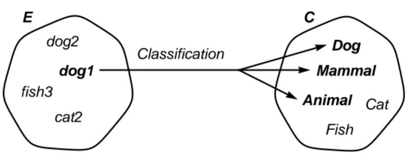
C, as depicted in Figure 17. That is, given the representation of an exemplar, the system

should to correctly determine which category the exemplar belongs to. More generally, classification could be described as answering the question “what kind of thing is e?”, where e denotes an exemplar. For example, the classification question “what kind of thing is dog1?” may produce the answer “Dog”.

Figure 17: Classification is a mapping from a set of exemplar vectors E to a set of

cate-gory vectors C

The exemplar may however belong to more than just one category, as is the case in Robins’ Coactivation Network which constructs an inheritance tree (see section 3.1) where a presented exemplar may belong to several categories at once, namely to catego-ries at different levels in the hierarchy. In this case, the system could correctly respond by indicating any of the Dog, Mammal or Animal categories when presented with the dog1 exemplar (as depicted in Figure 18).

Figure 18: Classification of the dog1 exemplar should indicate three categories

If the system is only able to respond by indicating a single category, which is the case for both the Coactivation Network and LVQ, a context must be provided which in-dicates which of the categories it should respond with. Without this context, the system

e1 e₂ e₃ ... E c1 c₂ c₃ c_m C Classification dog1 E Dog Cat Mammal Animal C Classification dog2 cat2 Fish fish3

could respond with the same category, e.g. Mammal, each time the dog1 exemplar is pre-sented. This is a correct answer, but we may also want the system to be able to respond by indicating the Dog or Animal category.

Robins solves this by adding a “centrality criterion” which indirectly specifies at what level the desired category is situated. More generally, this can be interpreted as pro-viding a context for the classification, indicating at what abstraction level the desired cat-egory resides, which makes classification in the presence of inheritance trees into the necessary one-to-one mapping. In the case of multiple inheritance or multiple dimensions, the context needs to be extended further to indicate on which dimension the desired cate-gory resides (see Robins, 1989a, section 5.6) in order to get a one-to-one mapping1.

By allowing the system to respond by indicating more than just one category, we escape these problems. The architecture can then handle multiple inheritance as well as multiple dimensions by indicating all applicable categories at once. This is the approach taken here. Using this approach, the context now defines which category units we are in-terested in, i.e. the observer is part of the classification process. A formal definition of classification would thus look like Equation 4.

(4)

The definition of the context CNTXT depends on the task. By not specifying a

con-1. While contexts are natural for specifying dimensions, e.g. “What nationality has Michael” vs. “What religion has Michael”, they are harder to define for multiple inheritance. For example. how do we specify what single answer we want to the question “What occupation has Michael”, where the answer is “Both student and employee”? One solution for this problem is to create a new category “StudentEmployee”, but this can be extremely costly when there are many combi-nations. For example, a person may be both “German” and “British”, having one parent from each country, or they may be “German” and “Italian”, “German” and “French”, “German” and “Polish”, etc.

text, the interpretation is that we are interested in all categories.

The traditional ANN approach to classification is through a feed-forward network with a set of input units and a set of output units. The pattern for the exemplar is presented on the input units and the pattern for the category is then produced, by the system, on the output units. In the simplest case, the input units are connected directly to the output units, through a set of connections which have individual weights. Such a network suffers from the linear separability problem in that it cannot encode a mapping which is not linearly separable, such as the XOR problem1, but as discussed in section 5.6 the system should only use linearly separable categories. A single layer network is thus used here for classi-fications.

The clusters of exemplar vectors are divided using decision lines, which determine whether each exemplar belongs to a category. Each category here has one decision line since each category is represented using a single output unit. An example of how the de-cision lines divides the representational space is shown in Figure 19.

The decision lines can either determine “all-or-nothing” membership or gradient membership depending on the activation function for the output units. If a threshold func-tion is used, exemplars which are on one side of the decision line typically generates the value 0.0 on the output unit and those on the other side of the decision line generates 1.0. This means that the exemplar either completely belongs to the category (1.0) or it does not (0.0). By instead using linear activation function for the output units, the exemplars can have different degrees of category membership, depending on the distance to the de-cision line.

1. The solution to this problem lays in adding a set of units between the input and output units, which are called hidden units since they are not modified nor interpreted by a human observer, i.e. they are “hidden in the black box”. The hidden units allows the system to regroup the exem-plars into clusters which are more relevant for the classifications which are to be learnt.

Figure 19: Decision lines in a ANN determine the classifications

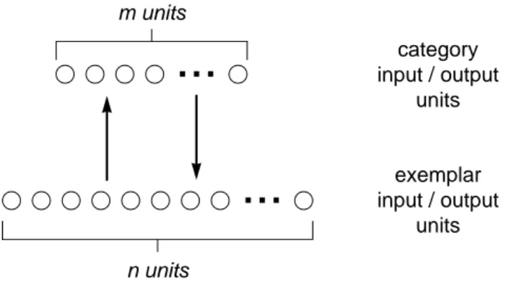
The classification mapping between exemplars E to categories C is done by con-necting the exemplar units to the category units with a set of connections. This leaves us with the classification architecture depicted in Figure 20. This architecture is the basis for our work; it is later (see section 4.3) extended to allow for prototype extraction and access.

Figure 20: A traditional classification network which maps exemplars encoded using n

units onto m categories where each category is represented by a single output unit

4.2.2 Prototype access

Prototype access is the process where a pattern of activation for a typical exemplar (the dog1 dog2 dog3 fish1 fish2 fish3 cat1 cat2 cat3 Cat Dog Fish

...

exemplar input units category output units n units

...

m units

prototype) is produced for a specified category. That is, it is a mapping from the set of categories C to the set of prototypes, represented as exemplar vectors E, as depicted in Figure 21.

Figure 21: Prototype access is mapping from a set of category vectors C to a set of

pro-totypes, represented using the exemplar vectors E

The process of accessing the prototype thus answers the question “what does a typ-ical c look like?”, where c denotes a category. A more formal definition of prototype ac-cess looks like Equation 5.

(5)

The classification mapping between exemplars E and categories C was done using a set of connections from the exemplar units to the category units (section 4.2.1). Con-versely, the prototype access mapping between categories C and exemplars (prototypes)

E could perhaps be done using connections from the category units to the exemplar units,

i.e. using connections in the other direction; we will show that this is the case.

Using the very simple single-layered network, depicted in Figure 22, we should thus be able to access the prototype for a category simply by activating its category unit and

e₁ e₂ e₃ ... E c₁ c₂ c₃ c_m C Prototype access prototypeaccess : C→E

allowing activation to flow through the set of connections. The pattern of activation formed on the exemplar units should be the average representation for the category exem-plars, i.e. the category’s prototype.

Figure 22: A prototype access network which should be able to produce the prototype

representation for any single category

In order for this to work, the prototypes must already have been extracted and stored in the connection weights. The pattern of activation formed on the exemplar (output) units should depict what a typical exemplar belonging to the activated category (input) unit looks like. The pattern of activation on the exemplar units is formed using the connections from the category units to the exemplar units; the activation level of each exemplar unit is directly determined by the weight (strength) of the connection which emanates from the active category unit. The other connection weights, of connections emanating from the other—inactive—category units, are irrelevant since they do not influence the activation level of the exemplar units. (The influence is the connection strength times the activation level—which there are set to zero.)

This means that the connections—or more specifically—the connection weights be-tween each category unit and the exemplar units must already store the prototype pattern for the category. That is, the network must have extracted information about the prototype

...

category input units exemplar output units n units

...

m units

and stored it in the connection weights. In the next section, we show how this extraction and storing in weights can be done in an ANN.

4.3 Extraction

Prototype extraction is the process by which the network creates/calculates the (exemplar) vectors used as prototypes1. This section describes how this can be done by exploiting the effects of back-propagation on one-to-many mappings.

4.3.1 Back-propagation and one-to-many mappings

Back-propagation (Rumelhart et al., 1986) is an error reducing learning technique which minimizes the difference between the network’s output and the target (i.e. the desired) output.

When the back-propagation learning technique is applied to classification networks, the network learns to produce a certain output every time a certain input is presented. For example, using the training set depicted in Table 2, the network can learn to classify dog exemplars into the Dog category, cat exemplars into Cat, and fish exemplars into the cat-egory Fish. This mapping is a one-to-one mapping from input to output patterns.

1. These prototypes are not used for classification, which is the case in LVQ (see section 3.2). Rather, it is the decision lines (section 4.2.1) which determine classifications. Not using the pro-totypes for classification—even though they “are there”—should be considered a valid approach, as indicated by Rosch (1978). She states that the presence of prototypes in a system does not imply restrictions on the processes nor on the representations used by the system.

Input Output

dog1 Dog

dog2 Dog