Mälardalen University Press Licentiate Theses No. 186
STATIC TIMING ANALYSIS OF PARALLEL
SYSTEMS USING ABSTRACT EXECUTION
Andreas Gustavsson
2014
School of Innovation, Design and Engineering
Mälardalen University Press Licentiate Theses
No. 186
STATIC TIMING ANALYSIS OF PARALLEL
SYSTEMS USING ABSTRACT EXECUTION
Andreas Gustavsson
2014
Copyright © Andreas Gustavsson, 2014 ISBN 978-91-7485-170-0
ISSN 1651-9256
Printed by Arkitektkopia, Västerås, Sweden
Abstract
The Power Wall has stopped the past trend of increasing processor through-put by increasing the clock frequency and the instruction level parallelism. Therefore, the current trend in computer hardware design is to expose explicit parallelism to the software level. This is most often done using multiple pro-cessing cores situated on a single processor chip. The cores usually share some resources on the chip, such as some level of cache memory (which means that they also share the interconnect, e.g. a bus, to that memory and also all higher levels of memory), and to fully exploit this type of parallel processor chip, pro-grams running on it will have to be concurrent. Since multi-core processors are the new standard, even embedded real-time systems will (and some already do) incorporate this kind of processor and concurrent code.
A real-time system is any system whose correctness is dependent both on its functional and temporal output. For some real-time systems, a failure to meet the temporal requirements can have catastrophic consequences. There-fore, it is of utmost importance that methods to analyze and derive safe estima-tions on the timing properties of parallel computer systems are developed.
This thesis presents an analysis that derives safe (lower and upper) bounds on the execution time of a given parallel system. The interface to the analysis is a small concurrent programming language, based on communicating and syn-chronizing threads, that is formally (syntactically and semantically) defined in the thesis. The analysis is based on abstract execution, which is itself based on abstract interpretation techniques that have been commonly used within the field of timing analysis of single-core computer systems, to derive safe timing bounds in an efficient (although, over-approximative) way. Basically, abstract execution simulates the execution of several real executions of the analyzed program in one go. The thesis also proves the soundness of the presented ana-lysis (i.e. that the estimated timing bounds are indeed safe) and includes some examples, each showing different features or characteristics of the analysis.
Acknowledgments
I would like to express my deepest gratitude to my advisors, Bj¨orn Lisper, Andreas Ermedahl and Jan Gustafsson, for accepting me as a doctoral student and also for their patience and invaluable guidance during my education so far. Without you, this thesis would not exist. A special thanks goes to Vesa Hirvisalo for putting a lot of energy and time into getting acquainted with, and suggesting improvements on, my research. Last, but far from least, I would like to thank everybody with whom I have shared many laughs and experiences during coffee breaks, trips, parties, after works and other activities. Thank you all!
The research presented in this thesis was funded partly by the Swedish Re-search Council (Vetenskapsr˚adet) through the project “Worst-Case Execution Time Analysis of Parallel Systems” and partly by the Swedish Foundation for Strategic Research (SSF) through the project “RALF3 – Software for Embed-ded High Performance Architectures”.
Andreas Gustavsson V¨aster˚as, October, 2014
Contents
1 Introduction 1
1.1 Real-Time Systems . . . 1
1.2 Execution Time Analysis . . . 3
1.3 Research Questions . . . 7 1.4 Pilot Study . . . 8 1.5 Approach . . . 9 1.6 Contribution . . . 11 1.7 Included Publications . . . 12 1.8 Thesis Outline . . . 13 2 Related Work 15 2.1 Static WCET Analysis . . . 15
2.2 Static WCET Analysis for Multi-Processors . . . 16
2.3 WCET Analysis Using Model Checking . . . 18
2.4 Multi-Core Analyzability . . . 19
3 Preliminaries 21 3.1 Partially Ordered Sets & Complete Lattices . . . 22
3.2 Constructing Complete Lattices . . . 24
3.3 Galois Connections & Galois Insertions . . . 26
3.4 Constructing Galois Connections . . . 30
3.5 Constructing Galois Insertions . . . 37
3.6 The Interval Domain . . . 39
4 PPL: A Concurrent Programming Language 43 4.1 States & Configurations . . . 45
4.2 Semantics . . . 47
vi Contents
4.3 Collecting Semantics . . . 57
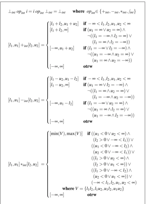
5 Abstractly Interpreting PPL 59 5.1 Arithmetical Operators for Intervals . . . 60
5.2 Abstract Register States . . . 60
5.3 Abstract Evaluation of Arithmetic Expressions . . . 63
5.4 Boolean Restriction for Intervals . . . 63
5.5 Abstract Variable States . . . 73
5.6 Abstract Lock States . . . 91
5.7 Abstract Configurations . . . 95
5.8 Abstract Semantics . . . 101
6 Safe Execution Time Analysis by Abstract Execution 155 6.1 Abstract Execution . . . 155
6.2 Execution Time Analysis . . . 177
7 Examples 181 7.1 Communication . . . 181
7.2 Synchronization – Deadlock . . . 186
7.3 Synchronization – Deadline Miss . . . 189
7.4 Parallel Loop . . . 190
8 Conclusions 197 8.1 The Underlying Architecture . . . 197
8.2 Algorithmic Structure & Complexity . . . 198
8.3 Nonterminating Transition Sequences . . . 202
8.4 The Research Questions . . . 203
8.5 Other Applications of the Analysis . . . 204
8.6 Future Work . . . 205
Bibliography 207
A Notation & Nomenclature 221
B List of Assumptions 225 C List of Definitions 227 D List of Figures 229 Contents vii E List of Tables 231 F List of Algorithms 233 G List of Lemmas 235 H List of Theorems 237 Index 239
vi Contents
4.3 Collecting Semantics . . . 57
5 Abstractly Interpreting PPL 59 5.1 Arithmetical Operators for Intervals . . . 60
5.2 Abstract Register States . . . 60
5.3 Abstract Evaluation of Arithmetic Expressions . . . 63
5.4 Boolean Restriction for Intervals . . . 63
5.5 Abstract Variable States . . . 73
5.6 Abstract Lock States . . . 91
5.7 Abstract Configurations . . . 95
5.8 Abstract Semantics . . . 101
6 Safe Execution Time Analysis by Abstract Execution 155 6.1 Abstract Execution . . . 155
6.2 Execution Time Analysis . . . 177
7 Examples 181 7.1 Communication . . . 181
7.2 Synchronization – Deadlock . . . 186
7.3 Synchronization – Deadline Miss . . . 189
7.4 Parallel Loop . . . 190
8 Conclusions 197 8.1 The Underlying Architecture . . . 197
8.2 Algorithmic Structure & Complexity . . . 198
8.3 Nonterminating Transition Sequences . . . 202
8.4 The Research Questions . . . 203
8.5 Other Applications of the Analysis . . . 204
8.6 Future Work . . . 205
Bibliography 207
A Notation & Nomenclature 221
B List of Assumptions 225 C List of Definitions 227 D List of Figures 229 Contents vii E List of Tables 231 F List of Algorithms 233 G List of Lemmas 235 H List of Theorems 237 Index 239
Chapter 1
Introduction
This chapter starts by introducing the fundamental concepts used within the field of the thesis. It then states the asked research questions, the approach used to answer the questions and the resulting contributions of the thesis. This chapter also presents the papers included in the thesis and a pilot study on using model checking for timing analysis of parallel real-time systems.
1.1 Real-Time Systems
As computers have become smaller, faster, cheaper and more reliable, their range of use has rapidly increased. Today, virtually every technical item, from wrist watches to airplanes, are computer-controlled. This type of computers are commonly referred to as embedded computers or embedded systems; i.e. one or more controller chips with accompanying software are embedded within the product. It has been approximated that over 99 percent of the worldwide production of computer chips are destined for embedded systems [15].
A real-time system is often an embedded system for which the timing be-havior is of great importance. More formally, the Oxford Dictionary of Com-puting gives the following definition of a real-time system [54].
“Any system in which the time at which output is produced is significant. This is usually because the input corresponds to some movement in the physical world, and the output has to relate to that same movement. The lag from input time to output time must be sufficiently small for acceptable timeliness.”
2 Chapter 1. Introduction
The word “timeliness” refers to the total system and can be dependent on me-chanical properties like inertia. One example is the compensation of temporary deviations in the supporting structure (e.g. a twisting frame) when firing a mis-sile to keep the mismis-sile’s exit path constant throughout the process. Another example is to fire the airbag in a colliding car. This should not be done too soon, or the airbag will have lost too much pressure upon the human impact, and not too late, or the airbag could cause additional damage upon impact; i.e. the inertia of the human body and the retardation of the colliding car both impact on the timeliness of the airbag system. It should thus be apparent that the correctness of a real-time system depends both on the logical result of the performed computations and the time at which the result is produced.
Real-time systems can be divided into two categories: hard and soft real-time systems. Hard real-real-time systems are such that failure to produce the com-putational result within certain timing bounds could have catastrophic con-sequences. One example of a hard real-time system is the above-mentioned airbag system. Soft real-time systems, on the other hand, can tolerate missing these deadlines to some extent and still function properly. One example of a soft real-time system is a video displaying device. Missing to display a video frame within the given bounds will not be catastrophic, but perhaps annoying to the viewer if it occurs too often. The video will still continue to play, although with reduced displaying quality.
The ever increasing demand for performance in computer systems has his-torically been satisfied by increasing the speed (clock frequency) and complex-ity (e.g. using pipelines and caches) of the processor. It is however no longer possible to continue on this path due to the high power consumption and heat dissipation that these techniques infer. Instead, the current trend in computer hardware design is to make parallelism explicitly available to the programmer. This is often done by placing multiple processing cores on the same chip while keeping the complexity of each core relatively low. This strategy helps increas-ing the chip’s throughput (performance) without hittincreas-ing the power wall since the individual processing cores on the multi-core chip are usually much simpler than a single core implemented on the equivalent chip area [89].
A problem with the multi-core design is that the cores typically share some resources, such as some level of on-chip cache memory. This introduces depen-dencies and conflicts between the cores; e.g. simultaneous accesses from two or more cores to shared resources will introduce delays for some of the cores. Processor chips of this kind of multi-core architecture are currently being used in real-time systems within, for example, the automotive industry.
To fully utilize the multi-core architecture, algorithms will have to be
par-1.2 Execution Time Analysis 3
allelized over multiple tasks, e.g. threads. This means that the tasks will have to share resources and communicate and synchronize with each other. There already exist software libraries for explicitly parallelizing sequential code au-tomatically. One example of such a library available for C/C++ and Fortran code running on shared-memory machines is OpenMP [83]. The conclusion is that concurrent software running on parallel hardware is already available today and will probably be the standard way of computing in the future, also for real-time systems.
When proving the correctness of, and/or the schedulability of the tasks in, a real-time system, it is, as far as the author knows, always assumed that safe (i.e. not under-approximated) bounds on the timing behavior of all tasks in the system are known. The timing bounds are, for example, used as input to algorithms that prove or falsify the schedulability of the tasks in the system [5, 34, 70]. Therefore, it is of crucial importance that methods for deriving safe timing bounds for this type of parallel computational systems are defined. This thesis presents a method that derives safe estimates on the timing bounds for parallel systems in which tasks share memory and can execute blocks of code in a mutually exclusive manner. The method mainly targets hard real-time systems. However, it can be applied to any computer system fitting the assumptions made in the upcoming chapters.
1.2 Execution Time Analysis
A program’s execution time (i.e. the amount of time it takes to execute the entire program from its entry point to its exit point) on a given processor is not constant in the general case; the execution time is dependent on the initial system state. This state includes the input to the program (i.e. the values of its arguments), the hardware state (e.g. cache memory contents) and the state of any other software that is executing on the same hardware. However, for any program and any set of initial states, at least one of the resulting execution times will be equal to the shortest execution time for the given program and set of initial states. The shortest execution time is referred to as the Best-Case Execution Time (BCET). Likewise, at least one of the resulting execution times will be equal to the longest execution time for the given program and set of initial states. The longest execution time is referred to as the Worst-Case Execution Time (WCET). Note that both the BCET and the WCET could
4 Chapter 1. Introduction 0 Time Probability Lower timing bound BCET Minimal observed execution time Maximal observed execution time WCET Upper timing bound The actual WCET
must be found or upper bounded
Measured execution times Possible execution times Derived bounds on the execution times
Worst-case performance Worst-case guarantee
Figure 1.1: Execution time distribution of some program. [113]
possibly be infinite,1though.
Figure 1.1 illustrates the relation between the possible execution times a program might have, and safe bounds on those execution times: any estima-tion of the WCET that is greater than the actual WCET is a safe bound on the actual WCET; likewise, any estimation of the BCET that is smaller than the actual BCET is a safe bound on the actual BCET. The figure also shows that measuring the execution time will always give a time between, and including, the BCET and WCET of the considered program. It is thus very difficult to guarantee that the actual BCET and WCET are found by measuring the execu-tion time of the program. This is since a huge number of possible initial system states must typically be considered in the general case.
When considering simple-enough (most often sequential) hardware, i.e. hardware that is free from timing anomalies [72], research on execution
time analysis can result in very efficient methods for tight (i.e. not too
over-approximate) estimation of the (BCET or) WCET. This is because tight estimations of the best-case and worst-case execution times for each single instruction, or a block of instructions, can be derived in isolation from other statements. However, when introducing multi-core architectures with 1One example for which both the BCET and WCET of a program are infinite is when the
program always enters some nonterminating loop along all possible paths. Another example of an infinite WCET is when a program deadlocks.
1.2 Execution Time Analysis 5
shared memory, the hardware does most likely suffer from timing anomalies regardless of how simple the processor cores are [2, 72, 97]. Practically, this means that an execution time for a statement that lies in-between the state-ment’s BCET and WCET could result in the global (BCET and) WCET. The consequence is that the only safe option is to take all the possible execution scenarios into account when estimating the global timing bounds.
Today, there exist several algorithms and tools that strive to derive a safe and tight estimate of the WCET of a sequential task targeted for sequential hardware. Some examples of such tools are aiT [30, 113], Bound-T [49, 113], Chronos [65, 113], Heptane [113], OTAWA [8], RapiTime [96, 113], SWEET [27, 113], SymTA/P [113] and TuBound [91, 113]. aiT, Bound-T and RapiTime are commercial tools while the others are primarily research pro-totypes. aiT, Bound-T, Chronos, Heptane, OTAWA and TuBound are purely static tools while SWEET and SymTA/P mainly use static WCET analysis techniques, but also dynamic techniques to some extent. RapiTime is heav-ily based on dynamic techniques.
In dynamic WCET analysis, measurements of the actual execution time of the software running on the target hardware are performed. This method is not guaranteed to execute the program’s worst-case path, though, which could, for example, include some error-handling routine that is only rarely executed. Thus, the WCET might be gravely under-estimated; i.e. there might exist paths through the code with considerably worse (longer) execution times than the worst execution time detected by the measurements.
In static WCET analysis, the program code and the properties of the target hardware are analyzed without actually executing the program. Instead, the analysis is based on the semantics of the programming language constructs used to define the program and a (timing) model of the target hardware. Static methods usually try to find a tight estimation of the WCET, but always safely over-estimate it.
Static WCET analyses are normally split into three subtasks: the flow
ana-lysis (formerly known as the high-level anaana-lysis), which constrains the possible
paths through the code; the processor-behavior analysis (formerly known as the low-level analysis), which attempts to find safe timing estimates for execu-tions of code sequences based on the considered hardware; and the calculation, where the most time-consuming path is found, using information derived in the first two phases. This is illustrated in Figure 1.2.
The flow analysis phase takes as input some form of representation of the analyzed program’s control flow structure (e.g. a Control Flow Graph, CFG [104]), and possibly additional information such as input data ranges and
6 Chapter 1. Introduction
Analysis steps Front
end CFG Flowanalysis
CFG & flow info Proc.-behavior analysis Local bounds Calc. Global bound WCET Exec.
program annot.User Analysis Input
Language
semantics Processormodel Tool construction
Figure 1.2: The three phases in traditional WCET analysis as commonly im-plemented in WCET analysis tools. [113]
bounds on the number of iterations for some loops. The additional informa-tion is often either provided manually by annotating the code, or derived using a preceding value analysis which statically finds information about the values of the processor registers and program variables etc. at every program point. The flow analysis outputs constraints on the dynamic behavior of the analyzed program, such as bounds on the number of loop iterations, (in)feasible paths in the control flow structure, dependencies between conditional statements, and which functions may be called.
The processor-behavior analysis phase takes as input the compiled and linked program binary and uses a model of the processor, memory subsystem, buses and all peripherals etc. to derive safe timing information for the execu-tion of the different instrucexecu-tions found in the program binary. The execuexecu-tion time of a given instruction is most often dependent on the occupancy state of the different hardware components; i.e. on the execution context. To derive tight timing information, it is therefore necessary to derive the possible execu-tion contexts for a given instrucexecu-tion; i.e. the possible hardware states in which the instruction can be executed. The processor-behavior analysis outputs such information.
For the calculation phase, there exist several possible strategies for com-bining the information retrieved from the flow analysis and processor-behavior analysis to derive a safe estimation of the WCET. These classes are further discussed and referenced in Section 2.1.
The traditional three-phase approach assumes that the analyzed program
1.3 Research Questions 7
consists of a single flow of control; i.e. is sequential. In a concurrent pro-gram, there are several flows of control (commonly referred to as threads or processes), possibly with dependencies among them. Such dependencies typ-ically occur when the threads or processes communicate or synchronize with each other. Thus, it should be obvious that problems such as race conditions, blocking of threads accessing shared resources, and deadlocks can occur. The consequence is that the processor behavior analysis is no longer compositional, which meas that the traditional three-phase approach is not directly applicable when analyzing arbitrary concurrent programs executing on parallel shared-memory architectures.
This thesis presents a static method that derives safe estimations of the BCET and WCET of a concurrent program consisting of dependent threads, for which race conditions, blocking of threads and deadlocks hence possibly can occur. The three traditional analysis phases are combined into one single phase; i.e. the method directly calculates the timing bound estimates while analyzing the semantic behavior of the program, based on a (safe) timing model of the underlying architecture. The definition of the timing model is out of the scope of this thesis but it is assumed to safely approximate the timing of all possible phenomena, including timing anomalies.
Note that solving the problem of finding the actual WCET in the general case is comparable to solving the halting-problem (i.e. determining whether the program will terminate), which is an undecidable problem (cf. [59]). Thus, the space of possible system states that a WCET analysis must search through could be extremely large, or even infinite, in the general case. This means that the analysis itself might not terminate in the general case. Therefore, techniques to increase the probability of, or even more desirable, guarantee, analysis termination must be derived. For many of the traditional methods for analyzing sequential programs, there are ways to guarantee termination using widening/narrowing techniques [81]. These techniques are not directly appli-cable to the method presented in this thesis, though. Therefore, other tech-niques will be presented.
1.3 Research Questions
This thesis mainly tries to answer the following questions. The overall question to be answered is Question 1. The other questions concern specific problems arising when analyzing concurrent programs consisting of dependent tasks.
8 Chapter 1. Introduction
Question 1: “How can safe and tight bounds on the execution time of a
con-current program consisting of dependent tasks be derived?”
Question 2: “How can the timing of synchronizing tasks be safely and tightly
estimated?”
Question 3: “How can programs suffering from deadlocks and other types of
nonterminating programs be handled?”
Question 4: “How can the timing of communicating tasks be safely and tightly
estimated?”
1.4 Pilot Study
Model checking is a technique for verifying properties of a model of some system. The idea of using model checking to perform WCET analysis has been investigated and shown to be adequate for analyzing parts of a single-core system [24, 52, 78].
Timed automata2can be used to model real-time systems [4]. An
automa-ton can be viewed as a state machine with locations and edges [57]. A state represents certain values of the variables in the system and which location of an automaton that is active, while the edges represent the possible transitions from one state to another [57]. (Continuous) time is expressed as a set of real-valued variables called clocks. UPPAAL3[9, 63, 111] is a tool used to model,
simulate and verify networks of timed automata [9, 10, 57].
Preceding the work presented in this thesis, an initial study [42] in which UPPAAL was used to model, and derive high precision estimates on the timing bounds of, a small parallel real-time system was performed. The paper shows that timing analysis of parallel real-time systems can be performed using the model checking techniques available in for example UPPAAL. However, the proposed method (i.e. the way the system was modeled and analyzed) did not scale very well, for example with respect to the number of threads in the an-alyzed program. Therefore, it was decided not to continue on the pure model checking path (although, there might be other ways to model the system that would succeed better).
2The formal syntax and semantics of timed automata can be found in [3] and [57].
3An introduction to UPPAAL and the formal semantics of networks of timed automata are
given in [9] and [57], respectively.
1.5 Approach 9
1.5 Approach
Abstract interpretation [23, 35, 81] is a method for safely approximating the
semantics of a program and can be used to obtain a set of possible abstract states for each point in the program. An abstract entity collects, and most often over-approximates, the information given by a set of concrete entities. An entity could for example be the value of a register – which in the abstract domain often is referred to as an abstract value; a collection of such information (e.g. a mapping from register names to their corresponding values) – which is often referred to as a state; or even a transition between states. By collecting the information given by a set of concrete entities into a single abstract entity, an analysis based on the abstract entities (i.e. an analysis based on abstractly interpreting the semantics of a program) can become less complex and more efficient, but might suffer from imprecision, compared to an analysis based on the concrete entities. Note that, in general, some form of abstraction of the concrete semantics has to be done since the analysis otherwise will become too complex due to the enormous number of entities/states that must otherwise be handled.
The concrete semantics of an arbitrary programming language can be ab-stracted in many different ways. The choice of abstraction is done by defining an abstract domain. An abstract domain is essentially the set of all possible ab-stract states that fit the definition of the domain. A provably safe abab-straction is often achieved by establishing a Galois connection between a concrete domain,
C, and an abstract domain, A, as depicted in Figure 1.3. A Galois connection
is basically a pair of two functions; the abstraction function,α, and the
con-cretization function,γ. The essence of Galois connections is that an abstraction
of a concrete entity always safely approximates the information given by the concrete entity: if an abstraction of a concrete entity within the concrete do-main is performed, followed by a concretization of the resulting abstract entity, then the resulting concrete entity will contain at least the information given by the original concrete entity. The details and properties of Galois connections are presented in Section 3.3.
The semantics of a program is basically a set of equations based on concrete states. A solution to these equations can be found by iterating on transitions between states until the least fixed point is found; this solution is often referred to as the collecting semantics of the program. Given a safe abstraction of the program semantics, the equations can always be defined and solved in the ab-stract domain. The resulting abab-stract solution is a safe approximation of the concrete solution (i.e. of the concrete collecting semantics).
10 Chapter 1. Introduction C c γ(a) A α(c) a α γ
Figure 1.3: Galois connection, α,γ , between a concrete (C) and an abstract (A) domain.
An example of an abstract domain isIntv, defined as {[z1,z2]| −∞ ≤ z1≤ z2≤ ∞ ∧ z1,z2∈ Z ∪ {−∞,∞}}; i.e. the set of all integer intervals that “fit
inside” [−∞,∞]. This domain can be used to over-approximate the concrete domain P({z ∈ Z∪{−∞,∞} | −∞ ≤ z ≤ ∞}) = P(Z∪{−∞,∞}); i.e. the set of all possible sets of integers between (and including) −∞ and ∞. In other words, a set of integers can be approximated using an interval. Note thatIntv is completely defined, and that a Galois connection is established betweenIntv and the concrete domain mentioned above, in Section 3.6.
Assume that the program variable x can have the value v, such that v ∈
{1,2,5,8}, in a given point of the program according to the concrete semantics
(i.e. x has four possible values in the given program point). In the abstract domain, the value of x could safely be represented by [1,8]. This is an over-approximation since turning the abstract value into a set of concrete values yields [1,8] → {1,2,3,4,5,6,7,8} ⊇ {1,2,5,8}. It can be noted that [1,8] is the best (tightest) approximation of the values of x, since [1,8] is the smallest interval containing all the possible concrete values of x.
Abstract execution (AE) [35, 40] was originally designed as a method to
derive program flow constraints [113] on imperative sequential programs, like bounds on the number of iterations in loops and infeasible program path con-straints. This information can be used by a subsequent execution time (WCET) analysis [113] to compute a safe WCET bound. AE is based on abstract in-terpretation, and is basically a very context-sensitive value analysis [81, 113] which can be seen as a form of symbolic execution [35] (i.e. sets of possible abstract values for the program variables etc. in the visited program points are found). Note that AE is in fact a technique for iterating on semantic transitions until a fixed point is found; i.e. a technique based on fixed point iteration. AE
1.6 Contribution 11
is very context-sensitive because the possible states at a specific program point considered in different iterations of the analysis do not necessarily have any obvious correlation to each other (e.g. the derived states of a given program point are not necessarily joined before used in future iterations). The program is hence executed in the abstract domain; i.e. abstract versions of the program operators are executed and the program variables have abstract values, which thus correspond to sets of concrete values.
The main difference between AE and a traditional value analysis is that in the former, an abstract state is not necessarily calculated for each program point. Instead, the abstract state is propagated on transitions in a way similar to the concrete state for concrete executions of the program. Note that since values are abstracted, a state can propagate to several new states on a single transition, e.g. when both branches of a conditional statement could be taken given the abstract values of the program variables in the current abstract state. Therefore, a worklist algorithm that collects all possible transitions is needed to safely approximate all concrete executions.
There is a risk that AE does not terminate. However, if it terminates then all final states of the concrete executions have been safely approximated [35]. Nontermination can be dealt with by setting a “timeout”, e.g. as an upper limit on the number of abstract transitions.
If timing bounds on the statements of the program are known, then AE is easily extended to calculate BCET and WCET bounds by treating time as a regular program variable that is updated on each state transition – as with all other variables, its set of possible final values is then safely approximated when the algorithm terminates [28].
The approach used in this thesis is to statically calculate safe BCET and WCET estimations by abstractly executing the analyzed program using a safe timing model of the underlying architecture. Basically, the only assumption made on the underlying architecture is that it provides (or can simulate) a shared memory address space, that can be used for communication, and shared resources, that can be used for synchronization. One example of such an archi-tecture is a multi-core CPU. Another example is a virtualization environment that runs on top of a distributed system and provides a shared memory view. Yet another example is any real-time operating system; e.g. VxWorks [115].
1.6 Contribution
12 Chapter 1. Introduction
1. PPL: a formally defined, rudimentary, concurrent programming lan-guage for real-time systems, including shared memory and synchro-nization on locks. The semantics of PPL includes timing behavior and is defined based on the familiar notation of operational semantics (cf. [82]).
2. An abstraction of the PPL semantics where values and concrete points in time are abstracted using intervals.
3. A safe timing analysis based on the abstract semantics of PPL. A com-plete correctness/soundness proof is provided.
1.7 Included Publications
This thesis includes the material presented in the following papers. Andreas Gustavsson is the main author of all the listed publications and has alone con-tributed with all the technical material presented in them.
Paper A
Worst-Case Execution Time Analysis of Parallel Systems
Andreas Gustavsson.
Presented at the RTiS workshop, 2011 [41].
This Paper addresses contribution 1 and presents the first definition of PPL and a very simple (non-generalized) timing model.
Paper B
Toward Static Timing Analysis of Parallel Software
Andreas Gustavsson, Jan Gustafsson and Bj¨orn Lisper. Presented at the WCET workshop, 2012 [43].
This Paper addresses contributions 2 and 3 and presents a work-in-progress timing analysis that can analyze all aspects of PPL, except synchronization. The presented analysis uses abstract execution to derive safe estimations of the BCET and WCET of the analyzed program.
1.8 Thesis Outline 13
Paper C
Toward Static Timing Analysis of Parallel Software - Technical Report
Andreas Gustavsson, Jan Gustafsson and Bj¨orn Lisper. Technical report, 2011 [44].
This Paper addresses contributions 2 and 3 and is an extended version of Paper B. The Paper includes all the mathematical details and a sketch for the correct-ness/soundness proof.
Paper D
Timing Analysis of Parallel Software Using Abstract Execution
Andreas Gustavsson, Jan Gustafsson and Bj¨orn Lisper. Presented at the VMCAI conference, 2014 [45].
This paper addresses contributions 1, 2 and 3 and summarizes the work pre-sented in this thesis. It presents a timing analysis that is based on the analysis defined in Papers B and C. The presented analysis derives safe estimations of the BCET and WCET for any program defined using a slightly modified version of PPL as presented in Paper A, given a (safe) timing model of the underlying architecture.
Paper E
Towards WCET analysis of multicore architectures using UPPAAL
Andreas Gustavsson, Andreas Ermedahl, Bj¨orn Lisper and Paul Pettersson. Presented at the WCET workshop, 2010 [42].
This paper does not address any of the main contributions of this thesis. How-ever, this paper contains the pilot study discussed in Section 1.4.
1.8 Thesis Outline
The rest of this thesis is organized as follows.
Chapter 2 presents some research that is closely related to the material pre-sented in this thesis. It also presents a brief introduction to the strategies traditionally used in WCET analysis.
Chapter 3 introduces the reader to the fundamental concepts and theories needed to understand the contents of the following chapters.
14 Chapter 1. Introduction
Chapter 4 formally defines PPL, a concurrent programming language. Chapter 5 presents a semi-safe abstraction of the PPL semantics. Note that
the abstraction is not safe for arbitrary PPL programs and that special care must be taken if using it (cf. Chapter 6).
Chapter 6 defines a safe timing analysis using abstract execution based on the abstraction made in Chapter 5.
Chapter 7 presents some examples that show how the analysis presented in Chapter 6 handles communication and synchronization in PPL programs.
Chapter 8 discusses the research questions and the analysis presented in Chapter 6. The chapter also gives pointers to future work.
For the reader’s convenience, the following appendices are provided. Appendix A summarizes the notations and nomenclature used in this thesis. Appendices B-H present listings of the assumptions, definitions, figures,
ta-bles, algorithms, lemmas and theorems defined in this thesis, respec-tively.
Chapter 2
Related Work
WCET-related research started with the introduction of timing schemas by Shaw in 1989 [104]. Shaw presents rules to collapse the CFG (Control Flow Graph) of a program until a final single value represents the WCET. This chap-ter presents some research related to this thesis and also to the traditional three-phase WCET analysis. Excellent overviews of the WCET research from the years 2000 and 2008 can be found in [92] and [113] respectively.
2.1 Static WCET Analysis
In this thesis, an approach for static analysis of the timing behavior of arbitrary concurrent programs based on threads, shared memory and synchronization on locks, as given by a small concurrent programming language, is presented. The field of static WCET analysis has, just until recently, mainly been focusing on sequential programs executing on single-processor systems. This is the kind of research referenced in this section.
In the field of processor-behavior (low-level) analysis, most research efforts have been dedicated to analyzing the effects of different hardware features, including pipelines [26, 47, 68, 105, 110], caches [66, 68, 110, 112], branch predictors [21], and super-scalar CPUs [67, 101].
Within flow (high-level) analysis, most research has been dedicated to loop
bound analysis. Flow analysis can also identify infeasible paths, i.e. paths
which are executable according to the program control flow graph structure, but not feasible when considering the semantics of the program and the
![Figure 1.1: Execution time distribution of some program. [113]](https://thumb-eu.123doks.com/thumbv2/5dokorg/4732852.125281/14.718.107.570.179.450/figure-execution-time-distribution-program.webp)