Mälardalen University Press Dissertations No. 176
MATHEMATICAL TOOLS APPLIED IN COMPUTATIONAL
ELECTROMAGNETICS FOR A BIOMEDICAL
APPLICATION AND ANTENNA ANALYSIS
Farid Monsefi
2015
School of Education, Culture and Communication Mälardalen University Press Dissertations
No. 176
MATHEMATICAL TOOLS APPLIED IN COMPUTATIONAL
ELECTROMAGNETICS FOR A BIOMEDICAL
APPLICATION AND ANTENNA ANALYSIS
Farid Monsefi
2015
Mälardalen University Press Dissertations No. 176
MATHEMATICAL TOOLS APPLIED IN COMPUTATIONAL ELECTROMAGNETICS FOR A BIOMEDICAL APPLICATION AND ANTENNA ANALYSIS
Farid Monsefi
Akademisk avhandling
som för avläggande av teknologie doktorsexamen i matematik/tillämpad matematik vid Akademin för utbildning, kultur och kommunikation kommer att offentligen försvaras tisdagen den 12 maj 2015, 13.15 i Delta, Mälardalens högskola, Västerås.
Fakultetsopponent: associate researcher Jean-Pierre Bérenger, LEAT Universite Nice Sophia Antipolis - CNRS
Akademin för utbildning, kultur och kommunikation Copyright © Farid Monsefi, 2015
ISBN 978-91-7485-200-4 ISSN 1651-4238
Mälardalen University Press Dissertations No. 176
MATHEMATICAL TOOLS APPLIED IN COMPUTATIONAL ELECTROMAGNETICS FOR A BIOMEDICAL APPLICATION AND ANTENNA ANALYSIS
Farid Monsefi
Akademisk avhandling
som för avläggande av teknologie doktorsexamen i matematik/tillämpad matematik vid Akademin för utbildning, kultur och kommunikation kommer att offentligen försvaras tisdagen den 12 maj 2015, 13.15 i Delta, Mälardalens högskola, Västerås.
Fakultetsopponent: associate researcher Jean-Pierre Bérenger, LEAT Universite Nice Sophia Antipolis - CNRS
Akademin för utbildning, kultur och kommunikation Mälardalen University Press Dissertations
No. 176
MATHEMATICAL TOOLS APPLIED IN COMPUTATIONAL ELECTROMAGNETICS FOR A BIOMEDICAL APPLICATION AND ANTENNA ANALYSIS
Farid Monsefi
Akademisk avhandling
som för avläggande av teknologie doktorsexamen i matematik/tillämpad matematik vid Akademin för utbildning, kultur och kommunikation kommer att offentligen försvaras tisdagen den 12 maj 2015, 13.15 i Delta, Mälardalens högskola, Västerås.
Fakultetsopponent: associate researcher Jean-Pierre Bérenger, LEAT Universite Nice Sophia Antipolis - CNRS
Abstract
To ensure a high level of safety and reliability of electronic/electric systems EMC (electromagnetic compatibility) tests together with computational techniques are used. In this thesis, mathematical modeling and computational electromagnetics are applied to mainly two case studies. In the first case study, electromagnetic modeling of electric networks and antenna structures above, and buried in, the ground are studied. The ground has been modelled either as a perfectly conducting or as a dielectric surface. The second case study is focused on mathematical modeling and algorithms to solve the direct and inverse electromagnetic scattering problem for providing a model-based illustration technique. This electromagnetic scattering formulation is applied to describe a microwave imaging system called Breast Phantom. The final goal is to simulate and detect cancerous tissues in the human female breast by this microwave technique.
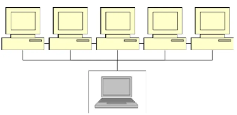
The common issue in both case studies has been the long computational time required for solving large systems of equations numerically. This problem has been dealt with using approximation methods, numerical analysis, and also parallel processing of numerical data. For the first case study in this thesis, Maxwell’s equations are solved for antenna structures and electronic networks by approximation methods and parallelized algorithms implemented in a LAN (Local Area Network). In addition, PMM (Point-Matching Method) has been used for the cases where the ground is assumed to act like a dielectric surface. For the second case study, FDTD (Finite-Difference Time Domain) method is applied for solving the electromagnetic scattering problem in two dimensions. The parallelized numerical FDTD-algorithm is implemented in both Central Processing Units (CPUs) and Graphics Processing Units (GPUs).
ISBN 978-91-7485-200-4 ISSN 1651-4238
Acknowledgements
I would like to extend my gratitude to the many people who helped me to accomplish this thesis. First and foremost, I would like to thank my supervisor Professor Sergei Silvestrov for his help, professionalism, valuable guidance and support throughout this project. I would also like to gratefully acknowledge my co-supervisor Dr. Magnus Otterskog for his continuous sup-port and encouragement in almost everything in my research work. I am really grateful to my co-supervisor Dr. Linus Carlsson for his support and numerous valuable conversations in theoretical concepts and also his accu-rate and insightful comments and suggestions about the thesis. I would like to express my deep sincere appreciation to Dr. Miliˇca Ranˇci´c for numerous conversations about electromagnetic modeling and a fruitful collaboration and also for her help and many valuable suggestions.
I have enjoyed the stimulating and friendly working atmosphere at UKK and IDT, M¨alardalen University. Special thanks to UKK’s Administration for their kind help and taking care of administrative issues. I wish to thank all my colleagues at the Division of Applied Mathematics at M¨alardalen University for their support and ideas. I am deeply indebted to Professor Anatoliy Malyarenko for his insightful comments about the thesis, valuable conversations and also Latex implementation of this work. Many thanks goes to Karl Lundeng˚ard, Christopher Engstr¨om and Jonas ¨Osterberg for so much help in many things. Special thanks to Hillevi Gavel for her accurate and careful corrections. I would also like to thank Alex Tumwesigye for his kind help in functional analysis and other related mathematical concepts. I am really grateful to my friend and colleague Dr. Nikola Petrovi´c at IDT and Per Olov Risman, for help and many valuable conversations in this research project. Many thanks goes also to Simon Elgland for a fruitful collaboration in the subject of parallelism.
I would express my sincere gratitude to Mathias Erlandsson who was the first one that presented the Mamacell project to me. Thanks to him I could start this interesting wonderful PhD project. I would also like to thank the 3
Mathematical Tools Applied in Computational Electromagnetics for a Biomedical Application and Antenna Analysis
RALF3 project funded by the Swedish Foundation for Strategic Research (SSF), not only for providing the funding which allowed me to undertake this research, but also for giving me the opportunity to attend conferences and meet so many interesting people. During this research I have had the pleasure to meet several people from the RALF3 project. Thank you for all brilliant ideas and conversations.
I would like to thank our family friends Rabizadegans, Modarresis and Liaghats, here in V¨aster˚as, for encouraging and supporting me and my fam-ily during these years of my research. I gratefully acknowledge my brother-in-law, Dr. Mahmoud Heyrat, for lot of fruitful conversations on Skype about Green’s functions and electromagnetism. I am grateful to my friend, Dr. George Fodor for his support and kindness and all the theoretical things I have learned from him.
I am deeply grateful to my brothers and sisters for their love, support and inspiration. As time goes on, I realize more and more clearly the huge impact that Eti and Aliashraf have had on my academic career and my life. I admire you all, each of you in a different way.
Last, but not least, I must express my very profound gratitude to my wife Fathieh and my children Navid and Nicki for providing me with unfailing support and continuous encouragement; for their sacrifice during my years of study and through the process of researching and writing this thesis. This accomplishment would not have been possible without you. Thank you my dearest family, I love you all.
I dedicate this thesis to the memory of my parents Badri Honarmand and Mohammadali Monsefi and my brother Said, whose role in my life was, and remains, immense.
V¨aster˚as, March, 2015 Farid Monsefi
4
This work was done in the frame of the RALF3 project funded by the Swedish Foundation for Strategic Research (SSF).
List of Papers
The present thesis contains the following papers:
Paper A. Monsefi, F., Ekman, J. (2006). Antenna analysis using PEEC and the com-plex image methods. In: Proceedings of the Nordic Antenna Symposium, Link¨oping, Sweden, 2006.
Paper B. Ekman, J., Monsefi, F. (2006). Optimization of PEEC based electromagnetic modeling code using grid computing. In: Proceedings of the EMC Europe
In-ternational Symposium on Electromagnetic Compatibility, Barcelona, Spain,
2006, 45–50.
Paper C. Monsefi, F., Ranˇci´c, M., Aleksi´c, S., Silvestrov, S. (2014). Sommerfeld’s in-tegrals and Hall´en’s integral equation in data analysis for horizontal dipole antenna above real ground. In: Proceedings of the 3rd Stochastic
Model-ing Techniques and Data Analysis International Conference - SMTDA 2014,
Lisbon, Portugal, 2014.
Paper D. Monsefi, F., Ranˇci´c, M., Aleksi´c, S., Silvestrov, S. (2014). HF analysis of thin horizontal central-fed conductor above lossy homogeneous soil. In:
Pro-ceedings of EMC Europe 2014, Gothenburg, Sweden, 2014, 916–921.
Paper E. Peri´c, M., Ili´c, S., Aleksi´c, S., Raiˇcevi´c, N., Monsefi, F., Ranˇci´c, M., Sil-vestrov, S. (2014). Analysis of shielded coupled microstrip line with par-tial dielectric support. In: Proceedings of XVII-th International Symposium
on Electrical Apparatus and Technologies - SIELA 2014, Bourgas, Bulgaria,
2014.
Paper F. Monsefi, F., Carlsson, L., Ranˇci´c, M., Otterskog, M., Silvestrov, S. (2014). Solution of 2D electromagnetic scattering problem by FDTD with optimal step size, based on a discrete norm analysis. In: Proceedings of 10th
Interna-tional Conference on Mathematical Problems in Engineering, Aerospace and Sciences - ICNPAA 2014, Narvik, Norway, 2014.
Paper G. Monsefi, F., Elgland S., Otterskog M., Ranˇci´c M., Carlsson L., Silvestrov, S. (2014). GPU Implementation of a Biological Electromagnetic Scattering Problem by FDTD. In: 16th ASMDA Conference Proceedings, 30 June-4
July 2015, Piraeus, Greece.
6
Parts of the thesis have been presented at the following international confer-ences:
1. The Nordic Antenna Symposium, Link¨oping, Sweden, May 30 - June 1, 2006. 2. EMC Europe International Symposium on Electromagnetic Compatibility,
Barcelona, Spain, September 6-9, 2006.
3. XVII-th International Symposium on Electrical Apparatus and Technologies - SIELA 2014, Bourgas, Bulgaria, May 29-31, 2014.
4. 3rd Stochastic Modeling Techniques and Data Analysis International Con-ference - SMTDA 2014, Lisbon, Portugal, June 11-14, 2014.
5. 10th International Conference on Mathematical Problems in Engineering, Aerospace and Sciences - ICNPAA 2014, Narvik, Norway, July 15-18, 2014. 6. EMC Europe 2014, Gothenburg, Sweden, September 1-4, 2014.
7. 16th ASMDA Conference, Piraeus, Greece, 2015.
Parts of the thesis have also been published in the following paper:
• Monsefi, F., Otterskog, M., Silvestrov, S., ”Direct and Inverse Computational Methods for Electromagnetic Scattering in Biological Diagnostics”,
Mathe-matical Physics (math-ph), Cornell University Library.
URL: http://arxiv.org/find/all/1/all:+AND+farid+monsefi/0/1/0/all/0/1
Contents
Papers A– E
1 Introduction . . . 9 2 Related Concepts in Electromagnetism . . . 14 3 Solution of Electromagnetic Fields and Antenna Analysis . . 34 4 Direct Electromagnetic Scattering Problem . . . 52 5 Inverse Electromagnetic Scattering Problem . . . 58 6 Medical Diagnostics and Microwave Tomographic Imaging by
Applying Electromagnetic Scattering . . . 72 7 Numerical Results and Conclusions . . . 80 8 Summaries of the Papers . . . 98
References 101
8
Introduction
1
Introduction
Almost any problem involving derivatives, integrals, or non-linearities can-not be solved in a finite number of steps and thus must be solved by a theo-retically infinite number of iterations for converging to an ultimate solution; this is not possible for practical purposes where problems will be solved by a finite number of iterations until the answer is approximately correct. Indeed, the major aspect is, by this approach, finding rapidly convergent iterative algorithms in which the error and accuracy of the solution will also be computed. In computational electromagnetics, a difficult problem like a partial differential equation or an integral equation will be replaced by, for instance, a much simpler system of linear equations. Replacing complicated functions with simple ones, non-linear problems with linear problems, high-order systems by low-high-order systems and infinite-dimensional spaces with finite-dimensional spaces are applied as other alternatives to solve easier problems that have approximately the same solution to a difficult mathe-matical model. Numerical modeling of electromagnetic (EM) properties are used in, for example, the electronic industry to:
1. Ensure functionality of electric systems. System performance can be degraded due to unwanted EM interference coupling into sensitive parts.
2. Ensure compliance with electromagnetic compatibility (EMC) regula-tions and directives. To prevent re-designs of products and ensure compliance with directives post-production.
3. Calculate EM properties of tissues inside the human body. To detect, for example, cancerous tissues.
Methods for determining electromagnetic field quantities, can be classified as experimental, analytical (exact), or numerical (approximate). The ex-perimental techniques are expensive and time-consuming but are still used. The analytic solution of Maxwell’s equations involves, among others, separa-tion of variables and series expansion, but are not applicable in the general case. The numerical solution of the field problems became possible with the availability of high performance computers. The most popular numeri-cal techniques are (1) Finite difference methods (FDM), (2) Finite element methods (FEM), (3) Moment methods (MoM), (4) Partial element equiva-lent circuit (PEEC) method. The differences in the numerical techniques have their origin in the basic mathematical approach and therefore make 9
Mathematical Tools Applied in Computational Electromagnetics for a Biomedical Application and Antenna Analysis
one technique more suitable for a specific class of problems compared to the others. Typical classes of problems in the area of EM modeling are:
• Printed circuit board (PCB) simulations (mixed circuit and EM prob-lem).
• Electromagnetic field strength and pattern characterization. • Antenna design.
• Microwave image reconstruction.
Further, the problems presented above require different kinds of analysis in terms of:
• Requested solution domain (time and/or frequency).
• Requested solution variables (currents and/or voltages or electric and/or magnetic fields).
The categorization of EM problems into classes and requested solutions in combination with the complexity of Maxwell’s equations emphasizes the importance of using the right numerical technique for the right problem to enable a solution in terms of accuracy and computational effort.
In many disciplines such as image and signal processing, astrophysics, acoustics, quantum mechanics, geophysics and electromagnetic scattering, inverse formulations are solved on a daily basis. The inverse formulation, as an interdisciplinary field, involves people from different fields within natural science. To find out the contents of a given black box without opening it by studying the input and output, would be a good analogy to describe the general inverse problem. Experiments will be carried on to guess and realize the inner properties of the box. It is common to call the contents of the box ”the model” and the result of the experiment ”the data”. The experiment itself is called ”the forward modeling”. As sufficient information cannot be provided by an experiment, a process of regularization will be needed. The reason to this issue is that there can be more than one model (’different black boxes’) that would produce the same data. On the other hand, ill-posed numerical computations will occur in the calculation procedure. Thus, a process of regularization constitutes a major step to solve the inverse problem. Regularization is used at the moment when selection of the most reasonable model is on focus. Computational methods and techniques ought to be as flexible as possible from case to case. A computational technique utilized for small problems may fail totally when it is used to large numerical 10
Introduction
domains within the inverse formulation. It is worth noting that ’small’ and ’large’ are relative concepts and they are changing rapidly with the progress of computer technology. A coefficient matrix of size of hundreds of millions can be considered large if one is using a high-performance computer while, similarly, a coefficient matrix of size of a few thousands can also be considered large if one is working on a workstation. Hence, methodologies and algorithms have to be created for new problems though existing methods are insufficient and computer technology is progressing rapidly. This is the major character of the existing inverse formulation in problems with large numerical domains. There are both old and new computational tools and techniques for solving linear and nonlinear inverse problems. When existing numerical algorithms fail, new algorithms must be developed to carry out nonlinear inverse problems.
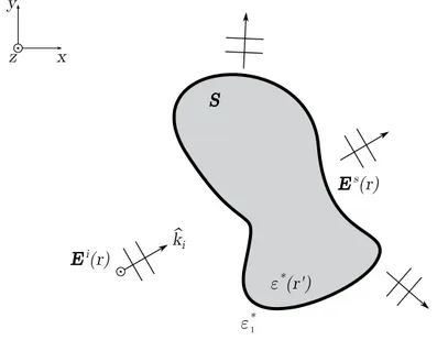
Electromagnetic inverse and direct scattering problems are, like other related areas, of equal interest. The electromagnetic scattering theory is about the effect an inhomogeneous medium has on an incident wave where the total electromagnetic field is consisted of the incident and the scattered field. The direct problem in such context is to determine the scattered field from the knowledge of the incident field and also from the governing wave equation deduced from the Maxwell’s equations. Even though the direct scattering problem has been thoroughly investigated, the inverse scattering problem has not yet a rigorous mathematical/numerical basis. Because the nonlinearity nature of the inverse scattering problem, one will face ill-posed numerical computation. This means that, in particular applications, small perturbations in the measured data cause large errors in the reconstruction of the scatterer. Some regularization methods must be used to remedy the ill-conditioning due to the resulting matrix equations. Concerning the ex-istence of a solution to the inverse electromagnetic scattering one has to think about finding approximate solutions after making the inverse problem stabilized. A number of methods is given to solve the inverse electromag-netic scattering problem in which the nonlinear and ill-posed nature of the problem are acknowledged. Earlier attempts to stabilize the inverse problem was via reducing the problem into a linear integral equation of the first kind. However, general techniques were introduced to treat the inverse problems without applying any integral equation formulation of the problem.
1.1
Background and Motivation
The vast and increasing applications of antennas within the electronic indus-try and biomedical applications desires constant mathematical analysis for 11
Mathematical Tools Applied in Computational Electromagnetics for a Biomedical Application and Antenna Analysis
one technique more suitable for a specific class of problems compared to the others. Typical classes of problems in the area of EM modeling are:
• Printed circuit board (PCB) simulations (mixed circuit and EM prob-lem).
• Electromagnetic field strength and pattern characterization. • Antenna design.
• Microwave image reconstruction.
Further, the problems presented above require different kinds of analysis in terms of:
• Requested solution domain (time and/or frequency).
• Requested solution variables (currents and/or voltages or electric and/or magnetic fields).
The categorization of EM problems into classes and requested solutions in combination with the complexity of Maxwell’s equations emphasizes the importance of using the right numerical technique for the right problem to enable a solution in terms of accuracy and computational effort.
In many disciplines such as image and signal processing, astrophysics, acoustics, quantum mechanics, geophysics and electromagnetic scattering, inverse formulations are solved on a daily basis. The inverse formulation, as an interdisciplinary field, involves people from different fields within natural science. To find out the contents of a given black box without opening it by studying the input and output, would be a good analogy to describe the general inverse problem. Experiments will be carried on to guess and realize the inner properties of the box. It is common to call the contents of the box ”the model” and the result of the experiment ”the data”. The experiment itself is called ”the forward modeling”. As sufficient information cannot be provided by an experiment, a process of regularization will be needed. The reason to this issue is that there can be more than one model (’different black boxes’) that would produce the same data. On the other hand, ill-posed numerical computations will occur in the calculation procedure. Thus, a process of regularization constitutes a major step to solve the inverse problem. Regularization is used at the moment when selection of the most reasonable model is on focus. Computational methods and techniques ought to be as flexible as possible from case to case. A computational technique utilized for small problems may fail totally when it is used to large numerical 10
Introduction
domains within the inverse formulation. It is worth noting that ’small’ and ’large’ are relative concepts and they are changing rapidly with the progress of computer technology. A coefficient matrix of size of hundreds of millions can be considered large if one is using a high-performance computer while, similarly, a coefficient matrix of size of a few thousands can also be considered large if one is working on a workstation. Hence, methodologies and algorithms have to be created for new problems though existing methods are insufficient and computer technology is progressing rapidly. This is the major character of the existing inverse formulation in problems with large numerical domains. There are both old and new computational tools and techniques for solving linear and nonlinear inverse problems. When existing numerical algorithms fail, new algorithms must be developed to carry out nonlinear inverse problems.
Electromagnetic inverse and direct scattering problems are, like other related areas, of equal interest. The electromagnetic scattering theory is about the effect an inhomogeneous medium has on an incident wave where the total electromagnetic field is consisted of the incident and the scattered field. The direct problem in such context is to determine the scattered field from the knowledge of the incident field and also from the governing wave equation deduced from the Maxwell’s equations. Even though the direct scattering problem has been thoroughly investigated, the inverse scattering problem has not yet a rigorous mathematical/numerical basis. Because the nonlinearity nature of the inverse scattering problem, one will face ill-posed numerical computation. This means that, in particular applications, small perturbations in the measured data cause large errors in the reconstruction of the scatterer. Some regularization methods must be used to remedy the ill-conditioning due to the resulting matrix equations. Concerning the ex-istence of a solution to the inverse electromagnetic scattering one has to think about finding approximate solutions after making the inverse problem stabilized. A number of methods is given to solve the inverse electromag-netic scattering problem in which the nonlinear and ill-posed nature of the problem are acknowledged. Earlier attempts to stabilize the inverse problem was via reducing the problem into a linear integral equation of the first kind. However, general techniques were introduced to treat the inverse problems without applying any integral equation formulation of the problem.
1.1
Background and Motivation
The vast and increasing applications of antennas within the electronic indus-try and biomedical applications desires constant mathematical analysis for 11
Mathematical Tools Applied in Computational Electromagnetics for a Biomedical Application and Antenna Analysis
new antenna structures. A good design of antenna, based on a mathemat-ical modeling, improves performance of an electronic device or system. In addition, to optimize the radiation energy in an advanced wireless system, the antenna serves as both a directional device and probing device. Anten-nas have a central role in the microwave technique in which the direct, and inverse electromagnetic scattering problem are solved in a system consisting of several antennas and wave-guides.
In order to guarantee operability of advanced electronic devices and systems, electromagnetic measurements should be compared to results from compu-tational methods. The experimental techniques are expensive and time con-suming but are still widely used. Hence, the advantage of obtaining data from tests can be weighted against the large amount of time and expense required to operate such tests. However, in some EM modeling applications like the scattering problem, information from both the numerical solution and experimental data is required and used in, for instance, a least-squares method. Analytic solution of Maxwell’s equations offers many advantages over experimental methods but applicability of analytical electromagnetic modeling is often limited to simple geometries and boundary conditions. Analytical solutions of Maxwell’s equations by the method of separation of variables and series expansions have a limited scope and they are not ap-plicable in a general case and rarely in a real-world application. Availability of high performance computers during the last decades has been one of the reasons to use numerical techniques within computational modeling to solve Maxwell’s equations also for complicated geometries and boundaries.
Scattering theory has had a major roll in twentieth century mathematical physics. In computational electromagnetics, the direct scattering problem is to determine a scattered field from knowledge of an incident field and the differential equation governing the wave equation. The incident field is emitted from a source, an antenna for instance, against an inhomogeneous medium. The total field is assumed to be the sum of the incident field and the scattered field. The governing differential equation in such cases is the coupled differential form of Maxwell’s equations, which will be converted to the wave equation.
In some applications, a model based illustration technique within the mi-crowave range is used to determine EM properties of biological tissues. Ap-propriate algorithms are used to make it possible for parallel processing of the heavy and large numerical calculation due to the inverse formulation of the problem. The parallelism of the calculations can then be implemented 12
Introduction
and performed on GPU:s, CPU:s, and FPGA:s. By the aid of a deeper math-ematical analysis and thereby faster numerical algorithms, an improvement of the existing numerical algorithms is expected. The algorithms may be in the the time domain, frequency domain and a combination of both domains. The main objective of this thesis is to apply mathematical modeling and algorithms for different antenna structures used in EMC applications and biological diagnostic technique. For EMC applications, radiation due to different antenna structures, above and in the proximity of the ground, is investigated. The ground has been assumed as both a perfect conductor and as a lossy medium. In comparison to situations where the ground is acting like a perfect conductor, more complicated mathematical models are desired to analyze antenna structures close to the ground as a lossy medium. In this thesis, this kind of problems are solved by both approximative and numeri-cal methods. For biomedinumeri-cal applications, the EM scattering formulation in two dimensions is solved and analyzed by finite difference approximations. The Finite Difference Time Domain (FDTD) method is used in this thesis to solve the two-dimensional electromagnetic scattering problem, first by a single processor. The electromagnetic scattering problem is, in fact, resem-bling a so-called Breast Phantom. The Breast Phantom is used to simulate human female breast by the microwave technology, detecting cancerous tis-sues in the breast. To speedup computational time, the FDTD algorithm is then parallelized by CPUs, GPUs, and FPGAs. The long computational time is a crucial issue when solving such kind of electromagnetic scattering problems. The new parallelized algorithms are developed and implemented in MATLAB and Octave to be re-programmed and executed in C, as a more optimized environment; this re-programming is done to suit the algorithms to GPU:s, CPU:s, and FPGA:s. The GPU parallelized algorithm is imple-mented in OpenCL and CUDA.
Mathematical Tools Applied in Computational Electromagnetics for a Biomedical Application and Antenna Analysis
2
Related Concepts in Electromagnetism
1 In constructing the electrostatic model, the electric field intensity vector
E and the electric flux density vector, D, are respectively defined. The fundamental governing differential equations are [10]
∇ × E = 0, (1)
∇ · D = ρv,
where ρv is the free charge density. By introducing = r 0 as the the electric permittivity where ris relative permittivity, and 0= 8.854× 10⁻¹²
F/m, the permittivity of the free space for a linear and isotropic media, E and D are related by relation
D = E. (2)
The fundamental governing equations for magnetostatic model are
∇ · B = 0, (3)
∇ × H = J,
where B and H are defined as the magnetic flux density vector and the magnetic field intensity vector, respectively. In the above, J is conducting current. B and H are related as
H = 1
µ0µrB, (4)
where µ0µr = µ is defined as the magnetic permeability of the medium
which is measured in H/m.; µ0 = 4π× 10−7 H/m is called permeability of space and µr is the relative magnetic permeability. The medium in
ques-tion is assumed to be linear and isotropic. Eqns. (1) and (3) are known as Maxwell’s equations in local form and constitute the foundation of elec-tromagnetic theory. As it is seen in the above relations, E and D in the electrostatic model are not related to B and H in the magnetostatic model. The coexistence of static electric fields and magnetic electric fields in a con-ducting medium causes an electromagnetostatic field and a time-varying magnetic field gives rise to an electric field. These are verified by numer-ous experiments. Static models are not suitable for explaining time-varying electromagnetic phenomenon. Under time-varying conditions it is necessary
1The following two chapters are based, to a large extent, on the work presented in [65].
14
Related Concepts in Electromagnetism
to construct an electromagnetic model in which the electric field vectors E and D are related to the magnetic field vectors B and H. In such situations, the equivalent equations are constructed as
∇ × E = −∂B ∂t, (5) ∇ × H = J +∂D ∂t , (6) ∇ · D = ρv, (7) ∇ · B = 0, (8)
where J is conducting current. As it is seen, the Maxwell’s equations above are in differential form. To explain electromagnetic phenomena in a physical environment, it is more convenient to convert the differential forms into their integral-form equivalents. To do this, the Stokes’s and divergence theorems can be applied. The Stokes’s theorem for an arbitrary vector A can be
written as C A· dl = S (∇ × A) · ds, (9)
which states that the circulation of a vector field A around a (closed) path C is equal to the surface integral of the curl of A over the open surface S bounded by C, provided A and ∇ × A are continuous on S. In Eqn. (9), quantities dl and ds are the infinitesimal length and surface, respectively. The divergence theorem, otherwise known as Gauss-Ostrogradsky, is stated
as [88] S A· ds = V (∇ · A)dv, (10)
which means that the volume integral of the divergence of a vector field equals the total outward flux of the vector through the surface that bounds the volume. In Eqn. (10), the volume V is enclosed by the closed sur-face S and dv and ds are the infinitesimal volume and infinitesimal sursur-face, respectively.
Now, based on the Stokes’s theorem, the integral form of Maxwell’s equations can be derived from the two Maxwell’s curl equations, stated in general form as [11, 25] ∇ × E = −Mi−∂B ∂t, (11) ∇ × H = Ji+ Jc+ ∂D ∂t, (12) 15
Mathematical Tools Applied in Computational Electromagnetics for a Biomedical Application and Antenna Analysis
2
Related Concepts in Electromagnetism
1 In constructing the electrostatic model, the electric field intensity vector
E and the electric flux density vector, D, are respectively defined. The fundamental governing differential equations are [10]
∇ × E = 0, (1)
∇ · D = ρv,
where ρv is the free charge density. By introducing = r 0 as the the electric permittivity where r is relative permittivity, and 0= 8.854× 10⁻¹²
F/m, the permittivity of the free space for a linear and isotropic media, E and D are related by relation
D = E. (2)
The fundamental governing equations for magnetostatic model are
∇ · B = 0, (3)
∇ × H = J,
where B and H are defined as the magnetic flux density vector and the magnetic field intensity vector, respectively. In the above, J is conducting current. B and H are related as
H = 1
µ0µrB, (4)
where µ0µr = µ is defined as the magnetic permeability of the medium
which is measured in H/m.; µ0 = 4π× 10−7H/m is called permeability of space and µr is the relative magnetic permeability. The medium in
ques-tion is assumed to be linear and isotropic. Eqns. (1) and (3) are known as Maxwell’s equations in local form and constitute the foundation of elec-tromagnetic theory. As it is seen in the above relations, E and D in the electrostatic model are not related to B and H in the magnetostatic model. The coexistence of static electric fields and magnetic electric fields in a con-ducting medium causes an electromagnetostatic field and a time-varying magnetic field gives rise to an electric field. These are verified by numer-ous experiments. Static models are not suitable for explaining time-varying electromagnetic phenomenon. Under time-varying conditions it is necessary
1The following two chapters are based, to a large extent, on the work presented in [65].
14
Related Concepts in Electromagnetism
to construct an electromagnetic model in which the electric field vectors E and D are related to the magnetic field vectors B and H. In such situations, the equivalent equations are constructed as
∇ × E = −∂B ∂t, (5) ∇ × H = J +∂D ∂t, (6) ∇ · D = ρv, (7) ∇ · B = 0, (8)
where J is conducting current. As it is seen, the Maxwell’s equations above are in differential form. To explain electromagnetic phenomena in a physical environment, it is more convenient to convert the differential forms into their integral-form equivalents. To do this, the Stokes’s and divergence theorems can be applied. The Stokes’s theorem for an arbitrary vector A can be
written as C A· dl = S (∇ × A) · ds, (9)
which states that the circulation of a vector field A around a (closed) path C is equal to the surface integral of the curl of A over the open surface S bounded by C, provided A and∇ × A are continuous on S. In Eqn. (9), quantities dl and ds are the infinitesimal length and surface, respectively. The divergence theorem, otherwise known as Gauss-Ostrogradsky, is stated
as [88] S A· ds = V (∇ · A)dv, (10)
which means that the volume integral of the divergence of a vector field equals the total outward flux of the vector through the surface that bounds the volume. In Eqn. (10), the volume V is enclosed by the closed sur-face S and dv and ds are the infinitesimal volume and infinitesimal sursur-face, respectively.
Now, based on the Stokes’s theorem, the integral form of Maxwell’s equations can be derived from the two Maxwell’s curl equations, stated in general form as [11, 25] ∇ × E = −Mi− ∂B ∂t, (11) ∇ × H = Ji+ Jc+∂D ∂t, (12) 15
Mathematical Tools Applied in Computational Electromagnetics for a Biomedical Application and Antenna Analysis
where Mi is the source magnetic current density (V /m2), Ji is the source
electric current density (A/m2), and Jc is the conduction electric current
density (A/m2). Taking the surface integral of both LHS and RHS of Eqn.
(11) yields [11] S (∇ × E) · ds = − S Mi· ds − ∂ ∂t S B· ds, (13)
which will be reduced to C E· dl = − S Mi· ds − ∂ ∂t S B· ds, (14)
by applying the Stokes’s theorem given in Eqn. (9). Eqn. (14) is referred to as Maxwell’s equation in integral form as derived from Faraday’s law which is stated as: The electromotive force appearing at the open-circuited terminals of a loop is equal to the time rate of decrease of magnetic flux linking the loop.
The corresponding integral form of Eqn. (12) can be written as C H· dl = − S Jic· ds + ∂ ∂t S D· ds, (15) in which Jic= Ji+ Jc (16)
Eqn. (15) is Maxwell’s equation in integral form as derived from Ampere’s law.
The procedure to obtain the integral form of the other two Maxwell equations, stated as
∇ · D = qev, (17)
∇ · B = qmv, (18)
in which qev is electric charge density (C/m3), and qmv is the magnetic
charge density (web/m3). The procedure to obtain the next integral form of
Maxwell’s equations is started by taking the volume integral of both sides of Eqn. (17), that is [11] V (∇ · D)dv = V qevdv (19)
By applying the divergence theorem, that is Eqn. (10), on the LHS of Eqn. (19), one can obtain [11]
S D· ds = V qevdv, (20) 16
Related Concepts in Electromagnetism
which is Maxwell’s electric field equation in integral form as derived from Gauss’s law, stated as: The total electric flux through a closed surface is equal to the total charge enclosed.
The divergence theorem, given by Eqn. (10) is applied on the LHS of
Eqn. (19) to obtain
S
B· ds = ρm, (21)
in which ρm is the total magnetic charge. Eqn. (21) is Maxwell’s magnetic
field equation in integral form as derived from Gauss’s law. In fact, there is no magnetic charge in nature but the concept is used as an equivalent to represent physical problems.
Maxwell’s equations in a more appropriate form to be applied in this work, are constructed as in the following table.
Maxwell’s equations
Differential form Integral form
∇ × H = J +∂D ∂t C H· dL = I + S ∂D ∂t · dS (22) ∇ × E = −∂B ∂t C E· dL = − S ∂B ∂t · dS (23) ∇ · D = ρv S D· dS = V ρvdv (24) ∇ · B = 0 S B· dS = 0 (25)
2.1
Green’s Functions
When a physical system is subject to some external disturbance, a non-homogeneity arises in the mathematical formulation of the problem, either in the differential equation, or in the auxiliary conditions, or both. When the differential equation is nonhomogeneous, a particular solution of the equation can be found by applying either the method of undetermined co-efficients or the variation of parameter technique. Green’s functions2 are specific functions that develop general solution formulas for solving non-homogeneous differential equations. Importantly, this type of formulation
2George Green, 1793-1841, was one of the most remarkable of nineteenth century physi-cists, a self-taught mathematician whose work has greatly contributed to modern physics.
Mathematical Tools Applied in Computational Electromagnetics for a Biomedical Application and Antenna Analysis
where Mi is the source magnetic current density (V /m2), Ji is the source
electric current density (A/m2), and Jc is the conduction electric current
density (A/m2). Taking the surface integral of both LHS and RHS of Eqn.
(11) yields [11] S (∇ × E) · ds = − S Mi· ds − ∂ ∂t S B· ds, (13)
which will be reduced to C E· dl = − S Mi· ds − ∂ ∂t S B· ds, (14)
by applying the Stokes’s theorem given in Eqn. (9). Eqn. (14) is referred to as Maxwell’s equation in integral form as derived from Faraday’s law which is stated as: The electromotive force appearing at the open-circuited terminals of a loop is equal to the time rate of decrease of magnetic flux linking the loop.
The corresponding integral form of Eqn. (12) can be written as C H· dl = − S Jic· ds + ∂ ∂t S D· ds, (15) in which Jic= Ji+ Jc (16)
Eqn. (15) is Maxwell’s equation in integral form as derived from Ampere’s law.
The procedure to obtain the integral form of the other two Maxwell equations, stated as
∇ · D = qev, (17)
∇ · B = qmv, (18)
in which qev is electric charge density (C/m3), and qmv is the magnetic
charge density (web/m3). The procedure to obtain the next integral form of
Maxwell’s equations is started by taking the volume integral of both sides of Eqn. (17), that is [11] V (∇ · D)dv = V qevdv (19)
By applying the divergence theorem, that is Eqn. (10), on the LHS of Eqn. (19), one can obtain [11]
S D· ds = V qevdv, (20) 16
Related Concepts in Electromagnetism
which is Maxwell’s electric field equation in integral form as derived from Gauss’s law, stated as: The total electric flux through a closed surface is equal to the total charge enclosed.
The divergence theorem, given by Eqn. (10) is applied on the LHS of
Eqn. (19) to obtain
S
B· ds = ρm, (21)
in which ρm is the total magnetic charge. Eqn. (21) is Maxwell’s magnetic
field equation in integral form as derived from Gauss’s law. In fact, there is no magnetic charge in nature but the concept is used as an equivalent to represent physical problems.
Maxwell’s equations in a more appropriate form to be applied in this work, are constructed as in the following table.
Maxwell’s equations
Differential form Integral form
∇ × H = J +∂D∂t C H· dL = I + S ∂D ∂t · dS (22) ∇ × E = −∂B ∂t C E· dL = − S ∂B ∂t · dS (23) ∇ · D = ρv S D· dS = V ρvdv (24) ∇ · B = 0 S B· dS = 0 (25)
2.1
Green’s Functions
When a physical system is subject to some external disturbance, a non-homogeneity arises in the mathematical formulation of the problem, either in the differential equation, or in the auxiliary conditions, or both. When the differential equation is nonhomogeneous, a particular solution of the equation can be found by applying either the method of undetermined co-efficients or the variation of parameter technique. Green’s functions2 are specific functions that develop general solution formulas for solving non-homogeneous differential equations. Importantly, this type of formulation
2George Green, 1793-1841, was one of the most remarkable of nineteenth century physi-cists, a self-taught mathematician whose work has greatly contributed to modern physics.
Mathematical Tools Applied in Computational Electromagnetics for a Biomedical Application and Antenna Analysis
gives an increased physical knowledge since every Green’s function has a physical significance. This function measures the response of a system due to a point source somewhere on the fundamental domain, and all other so-lutions due to different source terms are found to be superpositions 3 of
the Green’s function. Although Green’s first interest was in electrostatics, Green’s mathematics is nearly all devised to solve general physical prob-lems. The inverse-square law had recently been established experimentally, and George Green wanted to calculate how this determined the distribution of charge on the surfaces of conductors. He made great use of the electri-cal potential and gave it that name. Actually, one of the theorems that he proved in this context became famous and is nowadays known as Green’s the-orem. It relates the properties of mathematical functions at the surfaces of a closed volume to other properties inside. The powerful method of Green’s functions involves what are now called Green’s functions, G(x, x ). Applying Green’s function method, solution of the differential equation Ly = F (x), by L as a linear differential operator, can be written as
y(x) =
x
0
G(x, x )F (x )dx . (26)
To see this, consider the equation dy
dx+ ky = F (x),
which can be solved by the standard integrating factor technique to give y = e−kx x 0 ekx F (x )dx = x 0 e−k(x−x )F (x )dx , so that G(x, x ) = e−k(x−x )
. This technique may be applied to other more complicated systems. In general, Green’s function is the response of a system to a stimulus applied at a particular point in space or time. This concept has readily been adapted to quantum physics where the applied stimulus is the injection of a quantum of energy. Within electromagnetic computa-tion, it is common practice to use two methods for determining the Green’s
3Consider a set of functions φ
nfor n = 1, 2, ..., N . If each number of the functions φn
is a solution to the partial differential equation Lφ = 0, where L is a linear differential operator with some prescribed boundary conditions, then the linear combination φN =
φ0+
N
n=1
anφnalso satisfies Lφ = g. Here, g is a known excitation or source.
18
Related Concepts in Electromagnetism
function in the cases where there is some kind of symmetry in the geometry of the electromagnetic problem. These are the eigenvalue formulation and the Method of Images. These two methods are described in the following sections, but in order to its importance, the method of the eigenfunction expansion method is, first presented.
Green’s Functions and Eigenfunctions
If the eigenvalue problem associated with the operator L can be solved, then one can derive the associated Green’s function explicitly. It is known that the eigenvalue problem
Lu = λu, a < x < b, (27)
with prescribed boundary conditions, has infinitely many eigenvalues and corresponding orthonormal eigenfunctions as λnand φn, respectively, where
n = 1, 2, 3, .... Moreover, the eigenfunctions form a basis for the square integrable functions on the interval (a, b). Therefore it is assumed that the solution u is given in terms of eigenfunctions as
u(x) =
∞
n=1
cnφn(x), (28)
where the coefficients cn are to be determined. Further, the given function
f forms the source term in the nonhomogeneous differential equation Lu = f, u = L−1f
where L−1is the inverse operator to the operator L. Now, the given function
f can be written in terms of the eigenfunctions as f (x) = ∞ n=1 fnφn(x), (29) with fn= b a f (ξ)φn(ξ)dξ. (30)
Combining (28), (29), and (30) gives L ∞ n=1 cnφn(x) = ∞ n=1 fnφn(x). (31) 19
Mathematical Tools Applied in Computational Electromagnetics for a Biomedical Application and Antenna Analysis
When the linear property associated with superposition principle holds, it can be shown that [62]
L ∞ n=1 cnφn(x) = ∞ n=1 cnL(φn(x)). (32) But ∞ n=1 cnL(φn(x)) = ∞ n=1 cnλnφn(x) = ∞ n=1 fnφn(x), (33)
which finally yields L ∞ n=1 cnφn(x) = ∞ n=1 fnφn(x). (34)
By comparing the above equations, it will be obtained that
cn= 1 λn and fn= 1 λn b a f (ξ)φn(ξ)dξ for n = 1, 2, 3, .... (35) Further u(x) = ∞ n=1 cnφn(x) (36) = ∞ n=1 1 λn b a f (ξ)φn(ξ)dξ φn(x).
Now, it is supposed that an interchange of summation and integral is allowed. In this case, (36) can be written as
u(x) = b a ∞ n=1 φn(x)φn(ξ) λn f (ξ)dξ. (37)
On the other hand, by the definition of Green’s function, one may write
u(x) = L−1f = b a g(x, ξ)f (ξ)dξ. (38) 20
By comparing the last two equations, u(x) can be expressed in terms of Green’s functions as [62] g(x, ξ) = ∞ n=1 φn(x)φn(ξ) λn , (39)
where g(x, ξ) is the Green’s function associated with the eigenvalue problem (27) with the differential operator L.
2.2
Method of Images
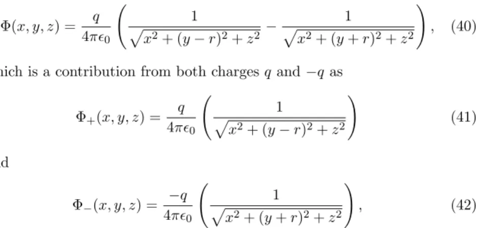
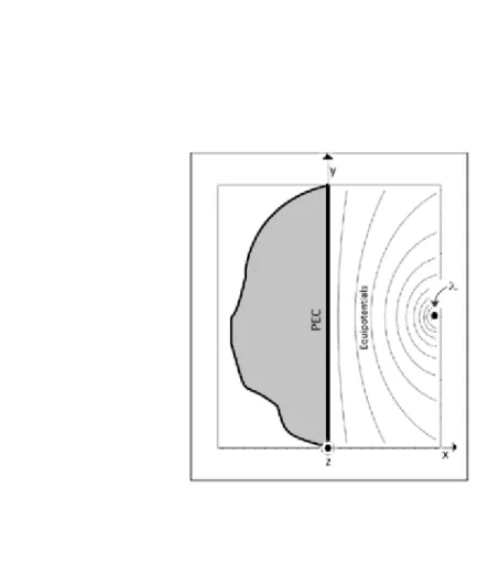
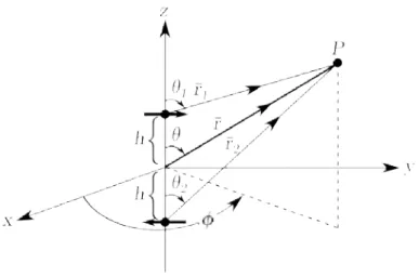
Solution of electromagnetic field problems is greatly supported and facil-itated by mathematical theorems in vector analysis. Maxwell’s equations are based on the Helmholtz’s theorem where it is verified that a vector is uniquely specified by giving its divergence and curl, within a simply con-nected region and its normal component over the boundary. This can be proved as a mathematical theorem in a general manner [6]. Solving par-tial differenpar-tial equations (PDE) like Maxwell’s equations, desires different methods, depending on, for instance, which boundary condition the PDE has and in which physical field it is studied. The Green’s function modeling is an applicable method for solving Maxwell’s equations for some frequently used cases with different boundary conditions. The issue in this type of formulation is, in the first hand, determining and solving the appropriate Green’s function by its boundary condition. Once the Green’s function is de-termined, one may receive a clue to the physical interpretation of the whole problem and hence a better understanding of it. This forms the general man-ner of applying Green’s function formulation in different fields of science. In some cases within electromagnetic modeling, where the physical source is in the vicinity of a perfect electric conducting (PEC) surface and where there is some kind of symmetry in the geometry of the problem, the Method of Images will be a logical and facilitating method to determine the appropriate Green’s function. The Method of Images can be used for the problems which include not only PEC surfaces but surfaces of materials with, for instance, dielectric characteristics or with finite specific conductance. The Method of Images is, in its turn, based on the uniqueness theorem verifying that a solution of an electrostatic problem satisfying the boundary condition is the only possible solution [24]. Electric and magnetic field of an infinitesi-mal dipole in the vicinity of an infinite PEC surface is one of the subjects that can be studied and facilitated by applying the Method of Images. In the following section, the Method of Images is applied to electromagnetic modeling of electrical sources above PEC surface.