Modern Portfolio Trading with Commodities

School of Sustainable Development of Society and Technology, Västerås NAA301 – The Bachelor Thesis in Economics (15 ECTS)

Spring Term, 2010

Modern Portfolio Trading

with Commodities

Supervisor:

Christos Papahristodoulou

Research Group:

Rahul Duggal

Date: 28 May, 2010

University: Mälardalen University, Västerås Campus, Sweden Programs: Analytical Finance (ANFI)

International Business Management (IBM)

Course: NAA301 – Bachelor Thesis in Economics (15 ETCS) Supervisor: Christos Papahristodoulou

Research Group: Spring Term, 2010

Rahul Duggal (rallee@hotmail.com)

Tawfiq Shams (tafic_87@hotmail.com)

Title: Modern Portfolio Trading with Commodities

Research Questions: What is the optimal portfolio weight composition between commodities and riskless asset for an investor with known and unknown risk preference?

Purpose: There is a big interest for alternative investment strategies than investing in traditional asset classes. Commodities are having a boom dynamic with increasing prices. This thesis is therefore based on applying Modern Portfolio Theory concept to this alternative asset class.

Methods: Basic statistical inference, Mean-variance optimization method, Excel, MATLAB

Conclusion: We managed to create optimal portfolios for investors with known and unknown risk preferences. When comparing expected returns to actual returns we found that for the investor with the known risk preference almost replicated the return of the markets. The other investor also profited but not as efficient as the market portfolio. Keywords: Mean Variance optimization, Absolute returns, Commodities,

First and foremost, I would like to thank my dear family and friends for their encouragement and support throughout my studies.

I would also like to acknowledge all my teachers who have provided me with knowledge that helped me writing this thesis.

-Tawfiq Shams

The first and foremost person I am going to thank is my late father Vijay Kumar Duggal who passed away in 2004. There are so many things I have learned and still carry from him. He is my biggest inspiration. Everything I do is for and because of him.

I would also like to thank my dear family and closest friends for everything they have supported me with.

-Rahul Duggal

Together we would like to thank Lars Pettersson (asset manager at IF Metall) who has been very helpful and supporting during our thesis work.

Finally, we would also like to express our great appreciation for the guidance and help we have received from our tutor, Christos Papahristodoulou. His aid and assistance has been really helpful to our work.

ABSTRACT ... II ACKNOWLEDGMENTS ... III

1 - INTRODUCTION AND OBJECTIVES ... 1

1.1–PROBLEM DISCUSSION ... 2

1.2–RESEARCH QUESTION ... 2

1.3-DATA AND METHODOLOGY ... 3

1.4–DELIMITATION ... 4

2 - OVERVIEW OF COMMODITIES ... 5

2.1-COMMODITY EXCHANGES ... 7

2.2-DYNAMICS OF THE COMMODITY MARKET ... 8

3 – SOME KEY DEFINITIONS AND STATISTICAL MEASURES ... 10

3.1–DEFINITIONS ... 10

3.2-GEOMETRIC VERSUS ARITHMETIC MEAN ... 10

3.3-VARIANCE AND STANDARD DEVIATION ... 11

3.4–HIGHER CENTRAL MOMENTS (SKEWNESS AND KURTOSIS) ... 12

3.5–PORTFOLIO’S EXPECTED RETURN AND RISK ... 14

3.6–DIVERSIFICATION ... 15

3.7–SHARPE RATIO ... 16

3.8-THE CAPITAL ALLOCATION LINE ... 17

4– MODERN PORTFOLIO THEORY ... 18

4.1-MEAN VARIANCE OPTIMIZATION ... 18

4.2-OPTIMAL PORTFOLIO AND THE INVESTMENT HORIZON ... 21

5 – UTILITY AND RISK AVERSION ... 22

5.1-THE COMPLETE PORTFOLIO DERIVATION (ALLOCATION BETWEEN THE RISKLESS AND THE RISKY ASSET) ... 24

6 – EMPIRICAL INVESTIGATION ... 27

6.1–DESCRIPTIVE STATISTICS ... 27

6.2–NORMALITY TEST -JARQUE-BERA ... 28

6.2.1 – Results ... 29

6.3-THE RISK FREE ASSET ... 29

6.4–FINDINGS OF PORTFOLIOS ON EFFICIENT FRONTIERS ... 30

6.5-EXPECTED RETURNS VSACTUAL RETURNS ... 33

7 - CONCLUSIONS ... 35

8 – REFERENCES ... 36

FIGURE 1-SHOW THE CLASSIFICATION OF COMMODITY SECTORS. ... 6

FIGURE 2-WEIGHT COMPOSITION IN DIFFERENT COMMODITY MARKETS IN MARCH 2008 ... 7

FIGURE 3-DIFFERENT STAGES OF SKEWNESS. ... 12

FIGURE 4-DIFFERENT STAGES OF KURTOSIS. ... 13

FIGURE 5–THE OPPORTUNITY LINE. ... 17

FIGURE 6-THE EFFICIENT FRONTIER. ... 18

FIGURE 7–CHARACTERISTICS ON THE FRONTIER ... 19

FIGURE 8-THE CAPITAL ALLOCATION LINE AND INDIFFERENCE CURVES. ... 23

FIGURE 9-EFFICIENT FRONTIER WITH COMPLETE PORTFOLIO ... 26

FIGURE 12-DEPICTION OF OUR WORK CREATED IN MATLAB. ... 33

FIGURE 11–RESULTING MEAN VARIANCE EFFICIENT FRONTIER... 45

FIGURE 12-SUGAR Q-Q PLOT AND DISTRIBUTION ... 47

FIGURE 13-LIVE CATTLE Q-Q PLOT AND DISTRIBUTION ... 47

List of Tables

TABLE 2–DESCRIPTIVE STATISTICS FOR THE ONE YEAR HOLDING PERIOD 2007-06-29 TO 2008-05-31. ... 27

TABLE 3–JARQUE-BERA TEST STATISTICS. ... 29

TABLE 4–CORRELATION VECTOR BETWEEN T-BILL AND ASSETS ... 30

TABLE 5–WEIGHT COMPOSITIONS OF PORTFOLIOS ... 31

TABLE 6–RISK-RETURN CHARACTERISTICS FOR EACH PORTFOLIOS ... 32

TABLE 7–EXPECTED AND ACTUAL RETURNS FOR PERIOD 2007-06-29 TO 2008-05-30(ONE YEAR HOLDING PERIOD). ... 33

1 - Introduction and Objectives

Commodity markets are seen as very complex and hard to understand. However, they are not that difficult. There are some basic facts that need to be known in order to understand the functions and nature of commodities. (Lerner, R 2000) The most inducing property of commodities as an asset class is that they are lacking or having a zero correlation to regular equities, which makes them attractive assets for diversified portfolios. (Lu and Almargo, 2009) In later years, the potential for profit creating investments in traditional asset classes has declined to various extents due to historically low interest rates and declining risk premiums. But on the other hand, there has been a boom dynamic within the commodities markets. An allocation to commodities offers a hedge against inflation. Commodity investments, in the long run, show equity-like returns and they are accompanied with lower volatility and shortfall risk. (Fabozzi, 2008, p.4) The Australian author Alan Heap describes in his article “China –The engine of a commodities super cycle” “that this growing trend is due

to the commodities super cycle theory, which is a lasting boom in real commodities usually due to urbanization and industrialization in major economies.” For instance, the re-building

of Europe after the Second World War distinguishes the super cycle theory. (Heap, 2005). However, in later years the prices have mostly been pushed by the heavily populated BRIC countries (Brazil, Russia, India and China). Chinas demand for industrial metals have been increasing between 70% to 90% in only a four years period (2001-2005) which has been a shock to the world wide demand and supply because of industrialization and urbanization. The average crude oil prices have been rising by 124% between the years of 2002-2006. But one should also be aware that the super cycle theory does not support a constant continuous growth phase. In 2006 it could be observed that many commodities lost approximately one fourth of its value due to economic pressures. (Fabozzi, 2008, p.4)

In general, there is a big discussion whether commodities are an asset class of their own compared to other asset classes. From definition the conditions for a market to be called an asset class is that an asset class consists of similar assets that have

 Homogenous risk-return profiles toward its own assets; that is they are highly correlated towards each other.

 Heterogeneous risk-return profiles towards other asset classes; which means low correlations towards other assets. (Fabozzi, 2008, p.7-9)

It should be acknowledged though that, like bankers or portfolio managers, individual investors and the commodity business also needs to follow the trend in the commodities universe while they decide on how to allocate their investments. For this purpose, there exist several Commodity Exchanges around the globe. These indices consist of collection of sub –indices exchange-traded funds (EFTs) from 4 different types of subsectors: Energy, Metals (precious and industrial), Agriculture and Livestock.

This paper will only study the US Standard & Poors Goldman Sachs Commodity Index (S&P GSCI), but we will briefly also talk about other commodity indices.

1.1 – Problem Discussion

There are many investment alternatives in the modern society. The most common ones are to invest in stock and bond markets. However, another alternative is to invest in the commodities markets and create wealth. In the 1950s, Professor Harry Markowitz introduced the Modern Portfolio Theory (MPT) where he showed how one can optimize investments by diversification of underlying portfolios consisting traditional asset classes. Is it possible to establish an optimized commodities portfolio in the same manner as with stocks or bonds? So the main purpose of this paper is to construct an optimal portfolio, using the MPT methods, consisting of only commodities for investors with known and unknown risk preferences. We will make an empirical study for 12 different commodities chosen from the S&P GSCI market for a time period between 2000-2007 and analyze the results whether it is appealing to invest or not. Further, a riskless asset will be introduced for the objective to either lend or borrow money to be able to create a more efficient investment horizon. We have a complete data set for the years 2000-2010 and hence we can compare return of our obtained portfolio (from the studied prediction period 2000-2007) to the actual returns for the out of sample period of 2007 to 2008 (that is, a holding period of one year) to see whether we have managed to create a better return than the market portfolio. All this will be discussed in more detail in section 1.4 Data and Methodology. We will also do some intermediate analysis to see if our framework fits in the MPT model since it assumes certain properties in the input arguments.

1.2 – Research Question

What is the optimal portfolio weight composition between commodities and riskless asset for an investor with known and unknown risk preference?

1.3 - Data and Methodology

The data to investigate consists of 12 risky commodities listed on the S&P Goldman Sachs Commodity Index (S&P GSCI), the S&P GSCI index itself and one risk-free government Treasury bill with one year to maturity. The commodities material was provided by the Chicago Board of Trade US and the government T-bill was ordered from the Federal Reserve System from the internet. (Federal Reserve System, 2010) There are two modifications to each of the commodity indices. The first one is that we ordered the data such that they are adjusted from future prices to spot prices. The second modification is that all the data are given in terms of points/ticks where each corresponding tick size-multiplier is given such that we can convert the points into dollar terms. For instance, Gold was quoted 719.53 points on 2008-10-31, with the tick-size multiplier of $100, we convert this into dollar terms and get that this is worth $71,953. The reason for different tick sizes is that each quoted number in terms of points represents one future contract size. For example, the 719.53 point represents one contract size of Gold for 100 ounces. To get the value in dollar terms we multiply this by its corresponding tick-size multiplier. See appendix 1 for each commodity tick-size multiplier. (Commodity trading system, 2008) Another important consequence with these adjustments is that one cannot buy proportions of the fixed commodity future contract sizes, which makes our optimized portfolio less possible to transact in real life. All data are given in terms of monthly close prices for the time period of 2000-04-28 to 2010-03-31. We decided to split this period into two different parts. Throughout this paper we will refer the first period to be called “The research period” which will be from 2000-05-31 to 2007-05-31. This is the period where are going to base our research on by applying statistical and MPT methods on. The second period will be called “The holding period” which will be from 2007-06-31 to 2008-05-31 which is the period where are holding our investment. The reason we chose these periods is because we didn’t want to include any crisis periods where the market trends diverges significantly too much from the expected trends. So we decided to exclude the financial crisis period that starts from around mid-2008.

There are three objectives that need to be obtained before we reach our final optimum portfolios. The first objective is to apply the Mean-Variance Optimization (MVO) method to our risky assets, commodities. This will give us efficient investment horizon of only commodities, where the weights to each commodity are the determining factors of each risk-expected return profiles. The second objective is to find the portfolio on this horizon with the maximum reward-to-variability from all the generated portfolios on the efficient frontier, called the Sharpe portfolio. This portfolio will be the suggested portfolio for an investor with an unknown risk preference. We will then introduce the riskless asset into our investment space such that we can create an even more efficient investment horizon. The last objective is to maximize utility for an investor with a fixed risk aversion and identify the appropriate portfolio (called the Complete Portfolio) for this objective.

We have mainly used two different computer softwares for different purposes, Microsoft Excel and MATLAB (Matrix Laboratory).

MATLAB is a programming language widely used by several industries and academic world. The program is mainly made for mathematical purposes that have many different applications and toolboxes. We have mostly been working with the “financial toolbox” and the “statistical toolbox”. There have been many different functions that we have used for our thesis, but the most important functions that we have used are frontcon and portalloc. The first functions solves for the quadratic problem to minimize risk and maximize returns for different weight compositions to create the efficient frontier while the latter function solves the problem to identifying the Sharpe Portfolio (optimal portfolio of only risky assets) and the Complete Portfolio (maximized utility portfolio). We will discuss these two functions in more detail later in this paper.

The other software, Microsoft Excel, has mostly been used for data handling and simpler calculations. We also had the possibility to upload excel files into MATLAB to be able to work with the programming more efficiently.

1.4 – Delimitation

1) Later in this paper we will work with utility functions and risk aversion coefficient, A, to connect an indifference curves to the mean variance space. The level of the risk aversion coefficient is a key assumption/limitation to our desired optimal portfolio.

2) In reality the central banks tends to change the risk free rate in order to adjust to economic conditions, which in turn creates some volatility to the riskless asset. We will assume that the risk or standard deviation of the risk less asset T-bill is zero to be able to work with the MPT model. It could be discussed whether this assumption should be valid or not since the risk free rates all over the world declined very sharply during the period

2000-2007.

3) Reliability of monthly returns. Since we are only handling monthly returns there can be some errors concerning the real return development of a commodity. Let us illustrate an extreme case to clear out our point. Let’s say that we have one commodity, for any specific month, that have had only positive returns for 30 days and on the 31th day of that month is registered to be negative. If this happens to frequently in a time series then we would, as consequence, calculate say, the geometric mean to be very low when in fact it is not. This is the downside of having only monthly returns with short time periods.

2 - Overview of Commodities

What kind of impact commodity markets has had throughout history is not fully known, but it has been pointed out that rice futures may have been traded in China 6000 years ago. It should be emphasized that shortages on critical commodities have sparked many wars throughout history. Examples are: in World War II, when Japan ventured into foreign lands in order to secure oil and rubber. Also, oversupply can have an overwhelming impact on a region by devaluing the prices of core commodities. Throughout history and in our modern times, commodity markets have had tremendous economic impact on nations and its people. It is known that ancient civilizations traded a wide selection of commodities. Such commodities were: livestock, seashells, spices and gold. Even if the quality of product, date of delivery and transportation methods were not reliable, commodity trading was an essential way of doing business. (Dumon, 2009)

Trading commodities are divided into four categories in order to be able to tell them apart. Each category includes commodities that have a certain particular property. These categories are as follows:

1. Energy (including crude oil, heating oil, natural gas and gasoline) 2. Metals (including gold, silver, platinum and copper)

3. Livestock and Meat (including lean hogs, pork bellies, live cattle and feeder cattle)

4. Agricultural (including corn, soybeans, wheat, rice, cocoa, coffee, cotton and sugar) (Dumon, 2009)

Since the quality of commodities is not standardized; every commodity has its own specific properties. An easy way to identify them is to distinguish between soft and hard commodities. Hard commodities are products from the energy, precious metals, and industrial metals sectors. Soft commodities are from the agricultural sector, such as grains, soybeans, or livestock, such as cattle or hogs and are usually weather-dependent, perishable commodities for consumption. (Fabozzi, Fuss, and Kaiser, 2008, p.6)

Figure 1 - Show the classification of commodity sectors. (Fabozzi et al, 2008, p.8)

Other important features of commodities are storability and availability (or renewability). Since storability plays a crucial role in pricing, we distinguish between storable and non-storable commodities. A commodity is said to have a high degree of storability if the cost of storage remains low with respect to its total value. Good examples are industrial metals such as aluminum or copper because they fulfill both criteria to a high degree. On the other hand, livestock is storable to only a limited degree since it is crucial for it to be continuously fed and housed at current costs, and is only profitable in a precise stage of its life cycle.

Then there are commodities which are nonrenewable such as silver, gold, crude oil, and aluminum. The supply of nonrenewable commodities depends on the producer’s ability to produce the raw material from the mines in both sufficient quantity and quality.

A factor that strongly influences the supply of commodities is the availability of commodity manufacturing capacities. For crude oil and some metals, the discovery and exploration of new reserves of raw materials is still an important issue. How to price nonrenewable resources depends strongly on current investor demand, while the pricing of renewable resources is more depended on estimated future production costs. (Fabozzi et al, 2008, p.7)

2.1- Commodity Exchanges

Commodity futures are traded at specialized exchanges that work as public marketplaces, where commodities are acquired and sold at fixed prices for fixed delivery dates. Commodity futures exchanges are typically structured as membership associations, where only members are allowed to trade. Transactions are made as standardized futures contracts by a broker who also is a member of the same exchange. It should be clear that a commodity exchanges main task is to provide an organized marketplace with uniform rules and standardized contracts. (Fabozzi et al, 2008. p 17-18)

US Standard & Poors Goldman Sachs Commodity Index

The Standard & Poor's Goldman Sachs Commodity Index (S&P GSCI) is recognized as a leading measure of general movements in prices in the world economy. The S&P GSCI provides investors with a reliable and publicly obtainable benchmark for commodity investment performance in the commodity markets. The index is designed to be tradable and is, primarily, calculated on a world production-weighted basis and is comprised of the principal physical commodities that are the subject of active, liquid futures markets. The weight of each commodity in the index is based on the average quantity of production as per the last five years of accessible data. The weights are chosen in a way so that they reflect the relative significance of each of the commodities in the world economy while preserving the tradability of the index. (Goldman Sachs, 2009)

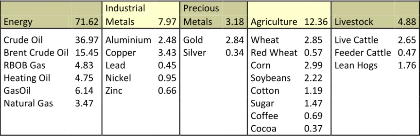
Figure 2 - Weight composition in different commodity markets in March 2008.

By looking at figure 2, it is obvious that S&P GSCI puts more weight focus in the energy sector while Dow Jones AIG has a more spread weight allocation. Below, one can see the precise weight composition in S&P GSCI.

Table 1 - Weight Composition in S&P GSCI in March 2008. (Goldman & Sachs, 2010)

2.2 - Dynamics of the Commodity Market

Investment capital market for commodities is used for the purpose of creating productive commodity capacity for the next coming generation. But there is a big difference in the supply-demand dynamics between the fungible commodities market and the investment capital commodities markets. The markets for the physical commodities have been cyclical and normal while the investment capital market for the commodities has been abnormal and non-cyclical. Generally in many cases, the commodity itself is easily accessible geologically but the capital to exploit it is restricted. The reason for this is of the political nature of the supplying countries. Since the 17th century political entities have been more interested in pursuing self interested intentions which has resulted in protectionism to several extents. The protectionism is created by constraining the free flow of capital, labor and technology by putting up higher costs/taxes to foreign countries or tariffs/subsidies to its own domestic country such that it becomes discouraging to make international investments. This in turn, results in a slowdown of commodity productive capacity around the world. The already existing productive capacity then suffers from physical shortages which, as consequence, pressure the prices of existing commodities upwards. Many have been concerned with the fact that rising prices in commodities have diverged from economic fundamentals of the physical commodities markets. This price rises however also reflects the need to motivate long-term investments to create more productive capacity since there is very high demand for hard commodities due to urbanization and industrialization around the world, especially from the BRIC-countries. Since protectionism restricts the ability to freely make investments in commodity related infrastructure, capital does not flow to the most efficient commodity investments, but rather to the most freely accessible one that is usually inefficient, extremely expensive and with poor rates of returns. The resulting excess capital that is not used in international investment is, in most cases, not redirected back to the industry at all and this creates a savings surplus which gives implications on the financial global markets. However, rather than redirecting the excess capital to, in some other way, Energy 71.62 Industrial 7.97 Precious 3.18 Agriculture 12.36 Livestock 4.88 Metals Metals

Crude Oil 36.97 Aluminium 2.48 Gold 2.84 Wheat 2.85 Live Cattle 2.65 Brent Crude Oil 15.45 Copper 3.43 Silver 0.34 Red Wheat 0.57 Feeder Cattle 0.47

RBOB Gas 4.83 Lead 0.45 Corn 2.99 Lean Hogs 1.76

Heating Oil 4.75 Nickel 0.95 Soybeans 2.22

GasOil 6.14 Zinc 0.66 Cotton 1.19

Natural Gas 3.47 Sugar 1.47

Coffee 0.69

infrastructural or production capacity investments, the capital is instead redirected to the financial sector to work out liquidity problems.

In general, the investment cycle can be divided into two phases that tends to recur every 20-25 years and last 10-15 years, that is the exploitation phase and the investment phase. (Goldman Sachs, 2008)

The exploitation phase: weak commodity prices and returns

The exploitation phase is the period where there are long periods of excess supply capacity and the utilization rates are high. This phase ends when the spare productive capacity is fully exhausted.

The investment phase: Rising costs and higher prices

The investment phase comes in the following period where investments are made to create productive capacity for the next generation of exploitation period.

Since year 2002 we have entered a new investment phase. All production capacity of hard commodities has been starved from the investments mainly made in the 1970s, which has resulted in the later year’s sharp rise in commodity prices. But due to the limited access to inputs and technology and a recent rise in protectionism, costs have also been forced up. This have resulted in a slowdown in the ongoing capacity expansion and again caused a re-acceleration of the price rises. This can also be seen on the S&P GSCI chart we have in appendix 4. Notice that the prices are rising but further accelerates around mid-2007.

3 – Some Key Definitions and Statistical Measures

In this section, different fields of the literature that are appropriate to this research will be identified and discussed.

3.1 – Definitions

Benchmark: Benchmark is a standard which the performance of securities, mutual funds or investments can be measured. Most often, broad market and market-segment stock and bond indexes are used for this purpose. It is important to compare an investment, when evaluating the performance of it, against an appropriate benchmark. In this paper we are using Standard and Poors Goldman Sachs Commodity Index (S&P GSCI) as our benchmark. (Jordan, B., Ross, S., and Westerfield, R, 2008, p. 71-72)

Short-selling: Short selling involves selling a security that the seller does not own. It can also involve any sale that is completed by the delivery of a security borrowed by the seller. Short sellers predict that the stock they are short selling will go down in price and they will be able to buy the stock at a lower amount than the price at which they sold short. (Levy and Post, 2005, p.71)

Value at Risk: Value at Risk is a concept that looks at the size of bad outcomes that can happen given the probability in a given time interval. In other words, this measures the potential loss that can occur from the mean given the probability of loss over some time period.

To be able to apply this concept one must assume a Gaussian distribution of the future returns. The formula for VaR is VaRE R( _i)Z_ 



3.2 - Geometric Versus Arithmetic Mean

Arithmetic Mean:

The arithmetic mean involves the sum of a list of numbers divided by the number of the items in that list. In other words, it is the average number of a list of numbers.

₁ 1 1 1 ( ... ) n A _{i n} i R R R R n  n 



Geometric Mean:

The geometric mean of returns is the compounded return changes of a set of data return series. 1 1

(1

)

1

R

R









According to Markowitz, it is more useful to use the geometric mean method when it comes to the calculations of the growth of a portfolio. Markowitz means that geometric mean will give a more accurate mean than arithmetic mean. Since geometric mean return is always less than the arithmetic mean return, the use of the expected return over-emphasizes the benefit of bearing increasing risk. Also, if the average of two extremes such 10000 and 0.0001 is compared, it is then obvious that geometric mean is more accurate than arithmetic because the geometric mean will be 1 while arithmetic will be 5000. (Geometric Mean, n.d)

3.3 - Variance and Standard Deviation

The variance and its square root, the standard deviation, are commonly used to determine the volatility of a stock or portfolio. Volatility is a statistical measure of the dispersion of return for a certain asset or market index. Volatility can be measured with either the standard deviation or variance between returns from that same security or market index. The larger the variance or the standard deviation is, the more spread out the return will be from the mean. Basically, the higher the volatility, the riskier is the asset or the index. (Levy and Post, 2005, p.715-716)

Variance:

The variance measures the averages squared difference between the actual returns and the average return. 2 2 1

1

(

)

1

s

R

R

n









Ri= the corresponding member of the data where i = 1, 2…n

R= The sample mean

This is only a general description of the variance, but since we are only working with the geometric sample mean in the MPT concept, we have that RRG.

The standard deviation:

The standard deviation of a sample of measurements is the positive square root of the variance.

The standard deviation is used as a measurement of risk. The lower standard deviation, the less volatile will the stock or portfolio is. (Jordan et al 2008, p. 382-384)

3.4 – Higher Central Moments (Skewness and Kurtosis)

Skewness

In our daily language, the word “skewed” refers to something that is out of line or distorted on one side. Skewness is a parameter that describes the asymmetry in a random variable’s probability distribution. More simply, it describes that a distribution is skewed if one of its tail is longer than the other. The distribution is positively skewed when high numbers are added to a normal distribution and the curve gets extreme scores on the right side. And a distribution is negatively skewed when the curve is pulled downward by extreme low numbers. Skewness can range from minus infinity to positive infinity. Skewness for a normal distribution is 0. (Wuensch, 2007 and Skewness, n.d) The formula for skewness is,

3 3 3 1 3 2 3/2 E ( ) E E ( )

[

]

[(

) ]

[

]

 is the third moment about the mean. (Wuensch, 2007) (Skewness, n.d) (Recall again that in our work we are only using the geometric sample mean.)

Kurtosis

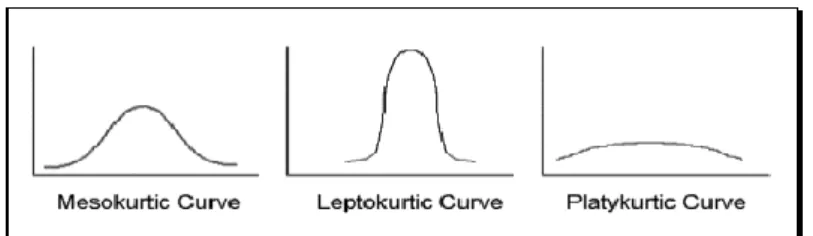
Kurtosis refers to the peakedness or flatness of a distribution. E.g. Kurtosis is a measure of how flat or peaked the top of a symmetric distribution is when it is compared to a normal distribution of the same variance. A normal curve or a normal distribution is measured as a perfect mesokurtic distribution. Curves or distributions that contain more score in the center than a normal curve tend to have higher peaks and are referred to as leptokurtic. Leptokurtic is also described as “fat in the tails” distribution. Distribution or curves that have fewer scores in the center than the normal curve and/or more scores on the outer slopes of the curve are said to be platykurtic. Platykurtic is often referred to as “thin in the tails” distribution. Kurtosis for a normal distribution is 3. The formula for kurtosis is,

where4_{is the fourth moment about the (geometric sample) mean. (Wuensch, 2007)}

Figure 4 - Different Stages of Kurtosis. (Kurtosis, n.d) 4 4 2 4 2 2 [( ) ] 3 3 [( ) ] E X E X           

3.5 – Portfolio’s Expected Return and Risk

The first thing to acknowledge is that the weights of the assets in the portfolio must sum up to 100%. Basically, the main tasks of portfolio managers are to determine the investment weights since investment weights are a decision variable.

The x represents weights of asset i in a portfolio that contains N assets. It is important to notify that when a portfolio involves short sales, weights can be negative. A portfolio which contains negative weights for some assets is called either a leveraged portfolio or borrowing portfolio. (Francis and Ibbotson, 2002, p.403)

A portfolio’s return is the sum of the weighted average of the expected returns of N assets:

Where the expected return of the portfolio is the security analysts forecast for expected rate of return from the ith asset. (Francis and Ibbotson, 2002, p.403-404)

It should be pointed out that expected return of a portfolio is based on forecast while the risk of a portfolio is calculated from historical data. The variance of the portfolio (risk) should be taken under consideration in two different ways, the first is that the variance represents the individual risks and the other is that it represents the interaction between N candidate assets. This equation is called the variance-covariance matrix:

Where and is a correlation coefficient between assets i and j. (Francis and Ibbotson, 2002, p.415-416)

3.6 – Diversification

Diversification helps an investor to manage risk and reduce the volatility of an asset’s price movements. Diversification is a technique, risk management uses, that mixes a wide variety of investments assets within a portfolio. The aim of diversification is to maximize return by investing in different investment assets that reacts differently to the same event. E.g. diversification minimizes the risk on a portfolio, but the return is not necessarily reduced. Funds that are recommended to invest in are often argued to be well-diversified. It is important to acknowledge that investment assets chosen within a portfolio do not have a perfect correlation but rather negative correlation. It should also be recognized that no matter how well diversified a portfolio is, risk can never be eliminated completely. (Fabozzi, 1999, p.398 and McWhinney, 2005) It is however important to understand the risk in order to be able to understand how to diversify. It should be noted that risk has two components, systematic and unsystematic. The sum of Systematic and unsystematic risk defines the total risk of a portfolio.

 Systematic risk, also known as, undiversifiable risk, where market forces affect the investment assets simultaneously in some systematic manner. Undiversifiable risk is associated with every company. Good examples are exchange rates, interest rates, political instability, War and changes in the level of inflation etc. Systematic risk is not connected to a company or an industry and cannot be eliminated or reduced throw diversification. (Fabozzi, 1999, p.399 and McClure, 2006)

 Unsystematic risk also known as, diversifiable risk is the other component of risk. The common sources of risk are business and financial risk. This risk is connected to a specific industry, market or a company and can be reduced throw diversification. Goods examples of unsystematic risks are Acts of God (hurricane or flood), inventions, management errors etc. The aim is to invest in various assets so that they all will not be affected by the same market events. (Fabozzi, 1999, p.399 and McClure, 2006)

To achieve superior diversification, one should not only diversify with different types of companies but also different types of industries. Assets in a portfolio, that are more uncorrelated, are better off. This is because different investment assets such as stocks and bonds will not react the same way to a market event and a combination of these assets will reduce the sensitivity of the portfolio to market swings. (McWhinney, 2005)

3.7– Sharpe Ratio

Sharpe ratio (Reward-to-Variability) was developed by William F. Sharpe and is a measurement for risk-adjusted returns that is often used to evaluate the performance of a portfolio. The Sharpe ratio can provide a clear image whether one portfolio is performing better comparable to another portfolio by making an adjustment for risk. A portfolio that reaps higher returns than its peers is a good investment only if it doesn’t come with additional risk. The better risk-adjusted a portfolios performance has been, the greater is a portfolio’s Sharpe ratio. The Sharpe ratio is defined by:

Where,

= Expected return of the portfolio = Risk free asset return

= the standard deviation of the portfolios return

Note that the numerator is the equity premium where it shows the how much excess return we can benefit above the risk free return. The simplicity of Sharpe ratio is the reason for its popularity.

If an investor chooses to go with a passive strategy, that is to replicate his or hers portfolio return with the market portfolio return, he or she will have a Sharpe ratio equal to the market Sharpe ratio.

Since, the Sharpe index shows how much additional return you can get by adding more volatility of holding the risky asset over a risk-free asset, it is then clear that the higher Sharpe ratio, the better is the portfolios performance. In isolation, Sharpe ratio of a portfolio means nothing. You need a market ratio to compare your portfolio (or several portfolios) with. The objective is to get a higher Sharpe ratio than the market Sharpe ratio. (Levy and Post, 2005, p.769-770)

3.8 - The Capital Allocation Line

The opportunity line is an investment horizon for two assets, one riskless asset and one risky asset (or portfolio). This line is obtained by the mean variance optimization for a two-asset portfolio; hence this line can also be called the efficient frontier between the two assets. This is a linear equation with the riskless asset being the y-intercept and the Sharpe ratio of the risky asset being the slope. The illustration in figure 5 is seen entirely from the riskless assets point of view. This investment horizon simply says that when we mix the two assets with different proportions we will move along the line. If we invest 100% in the riskless asset, we are lending money to, in case of treasury bills, to the government. The more weights of risky asset we include in our portfolio, the more risk we are taking, until we can reach the risky asset with 100%. It should be acknowledged that if we are investing more than 100%, we are borrowing money (or actually short selling riskless assets) to afford a greater proportion to the risky asset.

Figure 5 – The Opportunity Line. (Authors)

The opportunity line usually comes under two names, either Capital Allocation Line (CAL) or the Capital Market Line (CML) depending on the risky assets/portfolios characteristics. When the risky assets expected return-risk profile replicates the market’s we call it the CML. When it is not replicating, it is then simply called the CAL. (Levy and Post, 2005, p.296-297)

4– Modern Portfolio Theory

Modern portfolio Theory (MPT) is one of the most important and influential economics theories that deal with finance and investments. The Modern Portfolio Theory was developed by Harry Markowitz (born August 24, 1927) and was published in 1952 in the journal of finance under the name of “Portfolio Selection”. Later in 1959, He also published a book by the name of “Portfolio Selection: Efficient Diversification of Investments”. He decades later in 1990 received Sveriges Riksbank Nobel Prize in Economic Sciences for this work. What Harry Markowitz started back in the early 1960s was continued through the development of the capital market theory, whose final product, the capital asset pricing model (CAPM), allowed a Markowitz efficient investor to estimate the required rate of return for any risky asset (Markowitz, 1990).

Basically, what MPT says is that, it is not enough to take only one particular asset’s risk and return under consideration but rather investing in several assets with low correlations towards each other. This will give the portfolio advantages of diversification. Hence, the relevant objective in the MPT concept is to chose the right combination (or proportions) of these assets to the optimal portfolios. This problem is solved with the Mean-variance optimization model.

4.1 -Mean Variance Optimization

The basic idea behind this model is that one can create a whole set of portfolios that offers the maximum rate of return for any given level of risk, or alternatively, we can create portfolios that offer the minimum risk for any given level of return. When plotting all these portfolios in a return-risk graph we will get a convex curve, called the efficient frontier. This curve represents the investment horizon of efficient combinations of these assets. By looking at the graph below we are illustrating the MVO effect by assuming only two assets, say, a bond (low risk asset) and a stock (high return asset), both of them lying on the efficient frontier, or our investment horizon.

Now see that if we are investing 100% in bonds and 0% in the stock we are standing on the lower blue point. If we change these proportions by, say, 10%, we are going to stand somewhere further to the left on the frontier, with 90% bond and 10% stock. As seen graphically, this yields a lower risk, but also higher return. If we keep changing these proportions in the same manner we will lower our risk until a certain point where the risk starts to increase again. Conversely, this is called the diversification of unsystematic risk. You can notice that the risk is not eliminated fully due to the unsystematic part of the risk. The extent of how far we can diversify and eliminate unsystematic risk is determined by the correlation coefficient. The lower coefficient is between these two assets, the more we will be able to diversify “and stretch the frontier curve towards the y-axis”. In an unrealistic extreme case of, say, a correlation between these two assets being -1, then we would end up with two linear straight lines where both have the same y-intercept and different slopes. We would have then diversified away all the risk. However, in this paper we have 12 different assets (commodities) to perform the MVO for. The idea is still the same but more complexes. We will solve for this by using computer quadratic solving. (Brown et al, 2007, p.77). One important thing that we need to point out is that the efficient frontier is really made up of portfolios rather than individual assets. So when seeking the optimum portfolio, we consider all those portfolios along the efficient part of the frontier depending on the return-risk relationship that one investor has as target. Below we point out different characteristics for different points on the efficient frontier.

Figure 7 –Characteristics on the frontier. (Schmidt, 2008) Assumptions

Markowitz model, as many other models, is based on assumptions that need to be taken under consideration when dealing with MPT.

o Investors ask for maximizing the expected return of their total wealth. o All investors have the similar expected single period investment horizon.

o All investors are risk-adverse, which means that they only will accept a higher risk if they are compensated with a higher expected return.

o All markets are perfectly efficient.

Based on these assumptions, most of which are pretty much common sense, when comparing a single asset or a portfolio of assets, only assets or portfolios with the highest expected return at the same or lower risk level are considered as efficient. (Francis and Ibbotson, 2002, p.402)

Objectives and constraints

The main objective is to minimize risk with respect to every level of expected portfolio returns. This is a matter of a programming problem, since the objective function is in quadratic form for the weight allocation to each asset.

In this paper we will only work with two constraints. Firstly, we put constraint on each generated (optimal) portfolio’s risk to be minimized. Secondly, the weight, xi, allocation to each asset cannot be less than 0% (short sales restricted) or more than 100% (leverage restricted). In general terms we say that we are:

1 1

min

x x





( )

R

x E R



1

x





0

 

x

1

Inputs

 Expected Returns for all assets  Expected covariance matrix

 Number of portfolios to generate on the frontier

(In our work we created 250 portfolios to obtain a smoother efficient frontier).  Constraints on weights

Outputs

 Vector of efficient expected portfolio returns  Vector of efficient portfolio risks

Once this is obtained, we can create the efficient frontier by plotting all the returns versus the risk levels on the mean-variance space. (The MathWorks, 2010) See Appendix 6 for a more detailed description and short example for a simple portfolio using this function.

4.2 - Optimal Portfolio and the Investment Horizon

Once we have indentified all efficient portfolios we will now further indentify the most optimal portfolio from these. This is done by finding the one portfolio that possesses the highest reward-to-variability, or in other words, the highest Sharpe ratio. To be able to do this we are now going to introduce the riskless asset into the mean variance space. In this paper we are working with the Treasury bill (1-year maturity). So now the objective becomes

max P f P R R         .

Once this particular portfolio is found we will denote it the Sharpe Portfolio. This portfolio is the one portfolio that would be suggested to an investor with unknown risk preference, since it is judged to yield a moderate risk aversion coefficient level. (Brown et al, 2007, p.104-105)

At this point we are now standing with two alternatives investments, the riskless asset and the Sharpe portfolio. The question now is what investment horizon of combination is there between these two assets? The way to solve for this is basically the same as we did before, that is to find the efficient frontier by the MVO method. But since we are only dealing with two assets the whole objective is a lot easier. Nonetheless, we don’t need to bother to implement this into any MATLAB programming scripts and rather solve for it the following way. This will yield us the same outcome. We will simply draw a line from this the Sharpe portfolio to the riskless asset that will lie on the y-intercept, creating a straight line. Notice that the riskless asset becomes the y-intercept and the Sharpe ratio the slope of this linear equation. This equation is our investment horizon (or also efficient frontier) and is called the Capital Allocation Line.

P f f P

R

R

CAL

R













_{ }

_





We can now understand from this equation that that we can either invest some or all of our investments to the riskless asset (lend money to, in our case, the government) or invest 100% or more (leverage the Sharpe portfolio) in the Sharpe portfolio. Recall that if the Sharpe portfolio’s return replicates the market’s return, it is then called the market portfolio and the CAL will then be called the Capital Market line. Also, if one chooses to buy (that is to replicate) the market portfolio, then he or she is having a passive portfolio strategy. (Bodie, Kane, Marcus, Perrakis, and Ryan, 2008, p.184)

5 – Utility and Risk Aversion

Now the point is reached where the need to establish an optimal weight allocation between riskless asset and the Sharpe portfolio, tailored for a reasonable investor. It will of course be difficult for an asset manager to give his client the exactly correct portfolio combination without knowing his preferences. So what many financial theorists do is that they quantify the investors risk preference with respect to risk. The obtained quantity is denoted by the letter A, also called the Risk aversion coefficient. It is a matter of questioning the client and issue surveys and is a big matter in behavioral finance. The more risk avert an investor is, the more he or she will consider risk free investments, since there is less uncertainty with this strategy. But on the other hand, if one is less risk avert, he or she will accept higher risk with sufficiently higher expected return compensation, in other words, a higher risk premium for each additional risk level. (Bodie et al, 2008, p.173).

The discussion will now move further into how to use this risk aversion amount in order to be able to identify the optimal portfolio in the mean-variance-space. To do so, utility functions have been introduced, which is a way to assign a number to every possible asset combination such that more preferred asset combinations get assigned higher numbers than less-preferred. (Varian, 2008)

A very common utility function that is widely used by financial economists is 2

(

) 0.

)

0

(

E R

05

Utility







A



A = Risk aversion coefficient

E(R) = expected return on portfolio

p

 = risk or standard deviation of portfolio.

Firstly, by making observations to this model, one can begin to notice that the higher the risk aversion value, A, gets, the more it will penalize the whole utility score when subtracting

away the amount 2

0.005* *A _p . Secondly, one can observe that a higher expected return will contribute with a higher utility score, while simultaneously the higher risk level will lower it. Thirdly, if one would have only invested in a riskless asset he or she would yield a utility score equal to the expected return since the risk is equal to zero, making the last term vanish. So this specific utility function makes perfect sense.

The next step is to build an indifference curve that represents a fixed utility. The indifference curves are constructed by simply solving for E(R) and fix the utility score and the risk aversion and then put increments on the risk.

Required 2

( ) 0.005 _P

E R  U A

One will find several expected returns by each increment of risk, and at the same time maintain the same level of utility. An example of this is illustrated below.

Figure 8 - The Capital allocation line and Indifference Curves. (Authors)

The Capital Allocation Line has been added as well for immediate explanatory purposes of the indifference curve in the mean-variance space. Portfolio P in this graph is the optimal efficient Sharpe portfolio consisting of only risky assets (that has been obtained with the mean-variance analysis) that is tangent to the efficient frontier. This portfolio should be offered to investors regardless of their degree of risk aversion.

Now one should take a brief look at the indifference curves. The point where the indifference curve is tangent to the capital allocation line will be the overall optimal portfolio for investors given risk aversion. This portfolio is also called The Complete Portfolio. It should be emphasized that the indifference curve could end up below the Sharpe portfolio on the CAL with a significantly high risk aversion. In general, if one was risk-neutral, the indifference curve would rather be a straight line, and with a risk-loving attitude the curve is instead convex somewhere below the efficient frontier. (Bodie et al, 2008. P187-192)

5.1 - The Complete Portfolio derivation (Allocation between the

riskless and the risky asset)

So far the overall optimal portfolio has graphically been pointed out where it lies on the mean-variance space, but what is the specific asset combination at that point? Let’s start over from the beginning. So far the capital allocation line has been calculated which represents an investment opportunity set of combination of one riskless asset and one portfolio of risky assets (the optimal Sharpe portfolio). It is now important to decide what combination of the riskless asset and the risky Sharpe portfolio should be. What exact combination will give the highest utility? It will of course be the one where have a maximized utility. So let’s do that.

First let y denote the weight put in risky portfolio. Then one can form the equations for the complete portfolio, C.





P f

E(R )



yE R

(

)

 

1

y

E(R )

where one can see that he or she has risk premium in the last term for each additional weight allocation in y. One can further denote the risk to be

P

C

y







Solve for y and get that C P

y







Now substitute y into the first equation and obtain

p f f [E(R ) - R ] E(R )= R +C C P





This defines the Capital Allocation line in the mean-variance space. Notice that the slope is the Sharpe ratio (risk premium divided by the risk of risky portfolio (or, market portfolio). Now all the components needed exist in order to be able to maximize the utility function for the complete portfolio with respect to y.

y

Max

E R

(

) 0.0



0

5

×

A

×



Substitute in E(RC) and C that was just obtained

2 2

[ (

)

] 0.005

f P f P

y

Now continue with taking the derivative and equate it to zero 2 p f [E(R ) -R ] - 0.005A × 2y _P =0 U y   _ 

Now solve for y and get that

2

(

)

0.01

E R

R

y

A







This weight will be the optimal choice of investment in the risky portfolio according to a given risk aversion preference. Notice that if the risk aversion coefficient gets very large in the denominator, the whole expression will get closer to zero, meaning that the more risk averts an investor is, the less weight, y, he or she would put in the risky asset. In mathematical notations we say that

2

(

)

lim

0

0.01

E R

R

A







It is important to remember that any point on the left side of the Sharpe portfolio (where y<1) on the CAL means that one have included all or some weight allocation to the riskless assets together with the Sharpe portfolio. In case of T-bills you are actually lending some or all of your investment to the government. On the right side of Sharpe portfolio (where y>1) you are borrowing money (or short selling risk free asset) to afford a bigger quantity of the risky Sharpe portfolio than what an investor could have initially afford. This strategy is also called to leverage, which means that you are trying to amplify the return profits by placing yourself in a higher investment position. (Bodie et al, 2008, p. )

In MATLAB we used the function portalloc to find the Sharpe Portfolio and the Complete Portfolio. Here are the parameters,

Input parameters

- Vector of efficient expected portfolio returns - Vector of efficient portfolio risks

- Matrix of efficient expected portfolio weights. Output parameters

- Risk and return for Sharpe Portfolio - Risk and return for Complete Portfolio - Fraction of weights put in Sharpe Portfolio

It is important to emphasize that the inputs here are the outputs of the frontcon function that we considered earlier. See appendix 6 for a more detailed description and a short example for a simple portfolio.

Let’s now make a quick summary of the work. At first, individual assets were optimized to find the one portfolio that gives the best reward-to-variability, the Sharpe portfolio. Once this was done we introduced the riskless asset into our investment space. We created the investment horizon for the riskless asset and the Sharpe portfolio by connecting them together and formed a linear equation, the Capital Allocation Line. Thereafter the maximized utility portfolio (Complete portfolio) was found for an investor given his risk aversion. The graph below illustrates the whole idea.

Figure 9 - Efficient Frontier with Complete Portfolio. (Authors)

To keep things in order we must emphasize that we have not allowed any short sales in the Sharpe portfolio, that is 0 x_i 1. But we do allow short selling after we have obtained this portfolio when we introduce the riskless asset. The weight x is the weight parameter within the Sharpe portfolio while the weight y is the weight parameter between the riskless asset and the Sharpe portfolio. Be careful not to confuse these two!

6 – Empirical Investigation

The empirical analysis of commodity investing is based on exactly 7 years (or 84 months) that ranges from 2000-05-31 to 2007-05-31. We will apply all the techniques and methods that we have discussed so far to our data sets.

6.1 – Descriptive Statistics

The first step in the empirical analysis is to take each monthly price and calculate the percentage change from the previous month price.

1 1 t t t t P P R P    

Thereafter the descriptive statistics was extracted that characterizes each of the return distributions. Recall that we are going to have a holding period of the obtained portfolios of exactly one year (2007-06-31 to 2008-05-31) and we have therefore expressed both the risk and returns in years by annualizing them.

12

R

 

R

12

1

12



 





Descriptive

statistics

Skewness Kurtosis Min Max

Corn 10.62% 7.50% 25.77% 0.44 1.14 -15.70% 26.72% Wheat 12.91% 10.55% 22.72% 0.40 -0.49 -14.42% 16.51% Soybeans 9.36% 5.88% 26.69% -0.10 1.00 -22.72% 21.34% Coffee 6.88% 2.24% 31.58% 1.04 1.35 -14.73% 27.00% Sugar 9.06% 4.54% 30.60% 0.18 -0.36 -17.09% 21.85% Cotton 4.18% 1.36% 30.62% 0.47 0.24 -14.60% 26.28% Crude 17.36% 13.78% 27.47% -0.22 -0.37 -19.78% 19.51% Natural Gas 26.83% 13.53% 53.39% 0.49 0.07 -25.81% 42.43% Gold 13.44% 12.62% 14.12% 0.25 -0.07 -9.32% 12.43% Silver 17.44% 14.33% 25.81% -0.06 0.77 -23.44% 18.46% Live Cattle 5.47% 3.92% 17.58% -1.32 4.79 -23.05% 11.49% Lean Hogs 3.75% 1.13% 28.02% 0.12 0.21 -18.25% 22.16% S&P GSCI 14.34% 12.06% 22.17% -0.11 -0.15 -16.62% 15.84% T-bill 3.27% 3.24% 1.55% 0.57 -0.86 1.01% 6.09%

The T-bill in the last row is already given in annual terms, so we only needed to calculate the mean of all of the monthly returns for the T-bills. Recall that we are only concerned with the geometric mean in our investigation. From this data we can see that gold has the lowest risk and Silver have the highest returns, but also they have respectively very low return and high risk in them as consequence. The correlation matrix for this statistics will be listed in Appendix 2 from where we will refer to frequently throughout the empirical analysis. Also see appendix 5 for more details on what exchanges these commodities are traded on.

6.2 – Normality Test - Jarque-Bera

Since Markowitz assumes a normal distribution (also called Gaussian distribution) in the mean-variance framework, there is an importance to study the effects of non-normal distribution of the sample returns. Let us first understand why this is important. The standard deviation is a measurement of the up- and downswing deviations from the mean. In a normal distribution each z-value will have a corresponding probability occurrence value on the y-axis. If the curve gets significantly distorted one will end up with probability occurrence values that are erroneously concluded. Thus, if one is measuring the risk in terms of standard deviations from the mean, he or she needs to make sure that they have the right probability assigned for each occurrence. A sample of data will not always take on a perfect Gaussian distribution, so the concluding determination if a series is normally distributed or not is a matter of testing the data at a reasonable significance level to see at least how close it is to a normal one. Therefore, there exist many normality tests out there, such as the Lilliefors test or Kolmogorov–Smirnov test. But the use of Jarque-Bera test is preferred in this thesis since it takes into account the higher central moments, skewness and kurtosis. The Jarque-Bera test is a test of goodness-to-fit measure of departure from normality. The test is a joint-hypothesis test that is based on skewness and kurtosis. The null hypothesis is that both of the higher central moments are equal to or close to zero at a specified significance level. In other words this means that if the skewness and/or excess kurtosis deviate significantly from the value zero, there will be an increased Jarque-Bera statistics. So the higher the statistic one gets, the less normally distributed the sample is. Formula for JB:

2 2

(

3)

(

)

6

4

n

K

JB



S





We will use the significance alpha level of 5% to test our data in MATLAB with the function JBtest that returns the hypothesis result, JB-statistics and the significant p-value result. (Jarque and Bera, 1987)

6.2.1 – Results

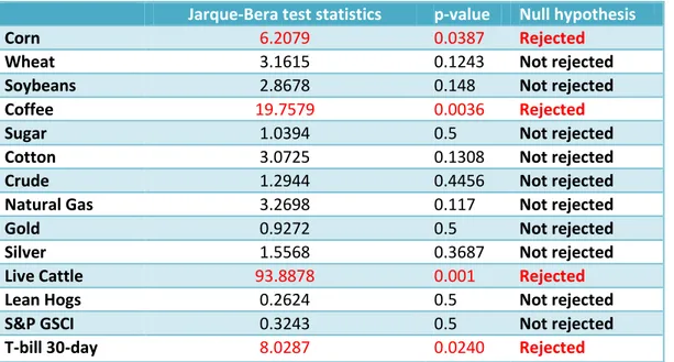
The results for the goodness to fit normal distributions have been very surprising. As we were expecting the majority of the monthly returns to have non-normal distributions we instead were proven to be wrong. Only 4 of the 15 datasets showed to be non-normally distributed. Let us discuss them in more detail.

Jarque-Bera test statistics p-value Null hypothesis

Corn 6.2079 0.0387 Rejected

Wheat 3.1615 0.1243 Not rejected

Soybeans 2.8678 0.148 Not rejected

Coffee 19.7579 0.0036 Rejected

Sugar 1.0394 0.5 Not rejected

Cotton 3.0725 0.1308 Not rejected

Crude 1.2944 0.4456 Not rejected

Natural Gas 3.2698 0.117 Not rejected

Gold 0.9272 0.5 Not rejected

Silver 1.5568 0.3687 Not rejected

Live Cattle 93.8878 0.001 Rejected

Lean Hogs 0.2624 0.5 Not rejected

S&P GSCI 0.3243 0.5 Not rejected

T-bill 30-day 8.0287 0.0240 Rejected

Table 3 – Jarque-Bera Test Statistics.

So we can observe that for each p-value being below the critical value of 5% significance level we reject the null hypothesis that the data set is normally distributed. See Appendix 7 for examples and illustration of rejected and non-rejected commodities.

6.3 - The Risk Free Asset

One of the most basic components in modern finance is the free rate of return. The risk-free rate is used by the capital asset pricing model and modern portfolio theory as the primary component from which other valuations are derived. The risk-free rate of return has a certain future result that can only be applied in theory. The risk-free rate of return is often used to evaluate whether one is being properly compensated for the additional risks that they are undertaking. The risk-free rate of return used is, traditionally, the shortest dated government Treasury bill (T-bills). T-bills are considered to be risk-free because they are backed by the government. (Schmidt, 2008) In our work we have indeed chosen the T-bill to be our riskless asset and we found that the average annual risk free rate is equal to 3.27%. As we can see in Table 2 there is 1.55% volatility in this riskless asset, and this is because in reality the central banks change their interest rates in accordance to the economic condition in various periods. The consequence will therefore be that the riskless asset is not really risk free. We will anyhow assume that the risk in our riskless asset (T-bill) is zero for us to be able