CDT 503 – Computer science, advanced level (15 hp)
School of Innovation, Design and Engineering
Master thesis
15 credits
Goran Brestovac and Robi Grgurina
Applying Multi-Criteria Decision Analysis
Methods in Embedded Systems Design
Västerås, Sweden
September 2013
ABSTRACT
In several types of embedded systems the applications are deployed both as software and as hardware components. For such systems, the partitioning decision is highly important since the implementation in software or hardware heavily influences the system properties. In the industry, it is rather common practice to take deployment decisions in an early stage of the design phase and based on a limited number of aspects. Often such decisions are taken based on hardware and software designers‟ expertise and do not account the requirements of the entire system and the project and business development constraints. This approach leads to several disadvantages such as redesign, interruption, etc. In this scenario, we see the need of approaching the partitioning process from a multiple decision perspective. As a consequence, we start by presenting an analysis of the most important and popular Multiple Criteria Decision Analysis (MCDA) methods and tools. We also identify the key requirements on the partitioning process. Subsequently, we evaluate all of the MCDA methods and tools with respect to the key partitioning requirements. By using the key partitioning requirements the methods and tools that the best suits the partitioning are selected. Finally, we propose two MCDA-based partitioning processes and validate their feasibility thorough an industrial case study.
Date: September 2013
Carried out at: MDH and ABB Corporate Research, Sweden Advisor at MDH: Gaetana Sapienza
Advisor at ABB: Gaetana Sapienza Examiner: Ivica Crnkovic
ACKNOWLEDGEMENTS
First of all we would like to thank Tihana Galinac Grbac, professor at Faculty of Engineering at University of Rijeka, for encouragement, advice and help for taking the opportunity to write our master thesis at the School of Innovation, Design and Engineering (IDT) at Mälardalen University (MDH).
Special thanks to Gaetana Sapienza our thesis supervisor at IDT for doing a splendid job at providing a lot of valuable advices, good ideas and a great guidance throughout the master thesis.
We would also like to thank Ivica Crnkovic, the master thesis examiner at MDH for providing a good environment, facilities for completing this master thesis, and all help and support while staying at MDH.
PREFACE
In today‟s industrial applications based on component design, some of the components may be implemented in software or in hardware based on a number of different and conflicting requirements. The decision impacts performance, power consumption, price, reliability and other system properties.
The system must fulfill all requirements taking into consideration all the constraints. Constraints could be project limitations like development time, budget, project deadline etc. or client strategic decisions like vendor loyalty. There are also a lot of interactions between components in the system which could lead to a multiple dependencies between them.
This leads to an optimization problem with multiple criteria. The criteria could be defined differently for software and hardware components. The criteria values for some components could be defined as ranges, might be missing or estimated. Multiple criteria decision analysis (MCDA) methods could be useful approach for solving the hardware/software partitioning problem.
Västerås, September 2013 Goran Brestovac
NOMENCLATURE
Abbreviation Explanation
AHP Analytic Hierarchy Process ANP Analytic Network Process CRSA Classical Rough Set Approach
DM Decision Maker
DRSA Dominance-based Rough Set Approach
ELECTRE ELimination Et Choix Traduisant la REalité (ELimination and Choice Expressing the REality)
ER Evidential Reasoning
HW Hardware
IDS Intelligent Decision System IT Information Technology
MCDA Multi-Criteria Decision Analysis MCDM Multiple-Criteria Decision-Making
NA Not Available
NS Not Specified
PROMETHEE Preference Ranking Organization Method for Enrichment Evaluations ROSE Rough Set Data Explorer
RSA Rough Set Approach
SMAA Stochastic Multicriteria Acceptability Analysis
SW Software
TOPSIS Technique for Order Preference by Similarity to Ideal Solution
VIKOR VIseKriterijumska Optimizacija I Kompromisno Resenje (Multicriteria Optimization and Compromise Solution)
CONTENTS
Chapter 1 INTRODUCTION 1
1.1 Motivation ...1
1.2 Research questions ... 2
1.3 Contribution ... 3
1.4 Structure of the Thesis ... 3
Chapter 2 PARTITIONING 4 2.1 Hardware/software partitioning ... 4
Related works ... 5
Chapter 3 MCDA METHODS 6 3.1 About MCDA ... 6 3.2 Ranking ... 8 AHP ... 8 ANP ... 14 TOPSIS ... 16 VIKOR ... 17 PROMETHEE I AND II ... 20 EVIDENTIAL REASONING ... 22 3.3 Classification ... 24 RSA ... 24 DRSA ... 27
3.4 Ranking and Classification ... 29
Electre III ... 29
Electre IV ... 31
ELECTRE TRI ... 33
SMAA-2 ... 34
SMAA-TRI ... 36
Chapter 4 MCDA TOOLS 37 4.1 Ranking ... 38
Electre III/IV ... 38
MakeItRational ... 39
ANP Solver ... 42
Web ANP Solver ... 43
TransparentChoice ... 44
Triptych ... 47
SANNA ... 48
Visual PROMETHEE Academic ... 49
Intelligent Decision System ... 52
4.2 Classification ... 55
Electre TRI ... 55
4eMka2 ... 56
jMAF ... 57
ROSE2 ... 60
4.3 Ranking and Classification ... 62
JSMAA ... 62
5.1 Partitioning process ... 65
5.2 Partitioning process requirements ... 66
5.3 Partitioning-driven criteria for evaluating the MCDA methods... 70
5.4 Partitioning-driven criteria for evaluating the MCDA tools ... 72
Chapter 6 RESULTS 74 6.1 Analysis and evaluation ... 74
MCDA methods evaluation ... 74
MCDA tools evaluation ... 74
Methods vs tools ... 74
Partitioning process requirements vs. Methods and Tools ... 75
6.2 MCDA-based partitioning process definition ... 77
Ranking ... 77
Classification ... 78
6.3 Wind turbine – case study ... 79
Ranking example – Visual PROMETHEE Academic & IDS ... 80
Classification example – 4eMka2 ...88
Chapter 7 DISCUSSION AND FUTURE WORK 90 7.1 Research questions ... 90
7.2 Future work ... 91
Chapter 8 CONCLUSION 92
Chapter 9 REFERENCES 93
Appendix A. Methods table 99
Appendix B. Tools table 104
Appendix C. 4eMka2 training examples 109
Chapter 1
INTRODUCTION
1.1 Motivation
In many industrial embedded systems an application could be implemented as software or as hardware executable unit. The process that determines if the application will be deployed as hardware or software is called partitioning. The partitioning process is of key importance to guarantee the application properties such as reliability, sustainability, efficiency, etc. Widely used approaches for carrying out the partitioning are based on hardware as well as software expertise, however they are not combined in synergic ways and the decisions are taken too early. As a consequence, this approach causes a number of issues such as redesign, interruption etc., which negatively affect the overall development process, the performance of the system and its lifecycle. Indeed, the decisions upon how the partitioning is carried out are very important because they affect many system properties. There are also several requirements that the system must satisfy. Additionally depending on the system size and complexity of the application there might be some dependencies between the components that have to be taken into consideration during the partitioning process.
According to the scientific papers the partitioning process is currently done based on a limited number of criteria. The partitioning is usually looked at as an optimization problem and is limited to few parameters. Parameters are usually hardware/software size, performance/timing constraints, power consumption and cost. These are the most important criteria but in practice there are a lot of other criteria that influence the partitioning process. The criteria are of different types (functional and non-functional) and some of the values could be missing or just estimated. Additionally, there might also be a number of existing components that could be reused instead of the development of the new ones. In this context it is of crucial importance to threat the partitioning problem from a multiple criteria perspective, in order to be able of taking partitioning decision on a large and even conflicting number of properties.
In this thesis we focus on defining the HW/SW partitioning process that could be used with a greater number of criteria utilizing existing MCDA methods and tools to help the decision-maker (DM) make the decision. In the process we take into consideration the reusability aspect, trying to find the best alternative from the set of existing component variants if they are available.
1.2 Research questions
In this section we introduce the research questions which have lead and guided this thesis work.
1. Could MCDA methods and tools be used for HW/SW partitioning?
Numerous MCDA methods and tools used both for ranking and classification have been proposed and studied, but only few of them have been applied to HW/SW partitioning process [1]. By answering two minor research questions (a, b) it will be also possible to answer to this main research question and find out which MCDA methods, tools and processes are able to satisfy the proposed HW/SW partitioning process requirements and what are their limitations.
a. What MCDA methods and tools exist and what are their characteristics? It is necessary to perform a systematic research and identify a number of HW/SW partitioning process requirements that will be used for evaluating MCDA methods and tools. For example, handling missing and qualitative values could represent the characteristics extracted from the requirements. Subsequently, the most suitable tools and methods with respect to the requirements for the partitioning process will be selected and applied to the wind turbine case study.
b. What kind of MCDA-based process could enable HW/SW partitioning?
We will examine and find out what kind of MCDA-based process could satisfy the HW/SW partitioning process requirements. For example, the scalability of the process (i.e. it must not be restricted to a limited number of units or alternatives) could represent one process requirement.
1.3 Contribution
In this thesis the hardware/software (HW/SW) partitioning processes that are able to handle a large number of criteria are proposed and presented on a practical example. To be able to do that the analysis of the MCDA methods and tools has been carried out. The partitioning process requirements have been identified and the key partitioning process requirements have been used in the evaluation of the MCDA methods and tools. Overall 14 methods and 14 tools have been analysed. The two partitioning processes have been created to enable the partitioning using the existing methods and tools. The first one is called the ranking process in which the existing component alternatives are available and the data is available for new hardware and/or software components. The second one is called the classification process in which the component is newly designed and there are no component alternatives available. In this case the component is defined by its criteria and the decision has to be made whether it is better to implement it as software or hardware. If the system consists of new and existing components, both processes could be used to partition the system, depending on the particular components. The ranking process could be used for partitioning components which have existing component alternatives to choose from, while the classification process could be applied in case of a new component for which there are no existing component alternatives to choose from. Both processes have been applied on the wind turbine case study.
1.4 Structure of the Thesis
This master thesis is organized as follows. The introduction to the thesis is provided in chapter 1. In chapter 2 the concept of partitioning process is introduced and the related works in the field are presented. Chapter 3 provides the background on the MCDA followed by the systematic research in which a number of the MCDA methods both for ranking and classification are identified. Chapter 4 provides the description of tools that implement these methods. The HW/SW partitioning process requirements are proposed in chapter 5. The number of the most important criteria are extracted from those requirements and used for evaluating the MCDA methods and tools. The final result of evaluation is presented in chapter 6 where the most suitable tools and methods for the partitioning process are selected. Two possible scenarios (i.e. ranking and classification scenarios) in the partitioning process are further proposed followed by the wind turbine case study of how processes work. Chapter 7 contains the discussion of the research questions and suggestions for the future work. The final conclusions are presented in chapter 8. Appendix A contains the methods table that consists of 14 MCDA methods and 32 criteria extracted from the HW/SW partitioning process requirements. Appendix B presents the tools table that consists of 14 MCDA tools and 27 criteria that are also extracted from the HW/SW partitioning process requirements. The ids file used for the wind turbine case study with the training data is presented in the Appendix C and the file with the testing data in the Appendix D.
Chapter 2
PARTITIONING
2.1 Hardware/software partitioning
The process for the development of systems that consist of software and hardware components is called hardware-software codesign. It deals with meeting the system requirements and trying to keep the project within time and budget constraints. In embedded systems some components might be implemented both in hardware and in software. Depending on the system and different component requirements, one of the two options has to be chosen. The hardware-software codesign is characterized by the concurrent development of hardware and software components.
For the system to be implemented, first the system specifications are defined. After thespecification process the system model is created. When the model is verified the HW/SW partitioning could be done. After the partitioning the software and hardware components are developed separately at the same time followed by the system integration and testing. Verification and validation are done in the end [2], [3].
The partitioning decisions are usually based on a limited number of criteria, usually hardware size, performance/timing constraints and power consumption. There are different approaches to the partitioning depending on the most important criterion and the number of criteria that are taken into consideration. In some cases it might be good enough to optimize one parameter, for example minimize the cost or hardware size while providing the acceptable level of performance.
Related works
There are many previous works done to HW/SW partitioning and numerous approaches like genetic algorithms [4], greedy heuristics [5], dynamic programming [6], simulated annealing algorithms [7] have been developed since the early 1990s.
One of these works models the Hardware Software partitioning problem as a Constraint Satisfaction Problem (CSP) [8].The near optimal solution is obtained by solving a CSP using the Genetic algorithm approach where three types of constraints (cost, timing and concurrecy) are considered.
Another paper presents two partitioning algorithms used in a HW/SW partitioning process [9]. The first one is an Integer Linear programming (ILP) based approach and the second one is genetic algorithm (GA). The partitioning problem is represented using the graph model in which nodes are the components of the system that have to be partitioned, and the edges represent communication between the components. Empirical tests have shown that the ILP-based solution works efficiently for graphs with several hundreds of nodes and produces the optimal solutions, whereas the genetic algorithm works efficiently for graphs of even thousands of nodes and gives near-optimal solutions.
The integer programming approach for solving the HW/SW partitioning problem and leading to (nearly) optimal results is also presented in another work [10]. This approach is based on the idea of „using the tools“ for cost estimation and nearly optimal results are calculated in short time beacuse the high computation time of solving IP-models is reduced by developing algorithm that splits the partitioning approach in two phases.
A technique for allocating hardware resources for partitioning has been proposed in another work [11]. The estimated HW/SW partition is built during the allocation algorithm. The components are taken one by one and then the most critical building block of the current component is allocated to hardware.
Chapter 3
MCDA METHODS
3.1 About MCDA
MCDA is an acronym that stands for Multiple Criteria Decision Analysis/Aiding, and it is sometimes referred as MCDM (Multiple Criteria Decision Making). It is a subdiscipline of operational research. Operational research is often considered to be a subfield of mathematics that applies advanced analytical methods to get optimal or near-optimal solutions in complex decision-making problems. Operational research is focused on practical problems in marketing, manufacturing, transportation, information technology (IT) and other fields. Therefore operational research overlaps with other disciplines, particularly operations management and engineering science. MCDA is a subdiscipline of operational research that explicitly deals with decision problems that use multiple criteria to determine the best possible solution [12].
The discipline was started in the 1960s and it evolved over time as new type of problems problem arose and had to be solved.
MCDA is applied in many fields like medicine, forestry, economics, management, transportation, etc. to solve a vast number of different problems. Indeed most decisions that are not easy to be taken, because they involve multiple and conflicting objectives. For instance:
Procurement: who is the best supplier? [13]
Key Performance Indicators: how to evaluate performance of business units? [14]
Portfolio Management: how to compose financial assets portfolio? [15]
Location: what is the best place to build a new facility (plant, warehouse, hypermarket, etc...)? [16]
Health Care: which criteria should be taken into account when introducing new technologies into the health care system? [17]
Sustainable Development: what is the best way to achieve sustainable development? [18]
In each case, one or several persons (DMs or stakeholders) have to compare different solutions (or actions) with several objectives in mind. For instance:
Procurement: minimize the price paid, maximize the quality of the product purchased, etc.
Key Performance Indicators: minimize costs, maximize profit, etc. Portfolio Management: minimize risk, maximize expected return, etc. Location: minimize investment cost, maximize expected return, etc.
Health Care: maximize efficiency, minimize side effects, etc.
Sustainable Development: reduce environmental impacts, reduce social impacts, etc. The degree of achievement of these objectives can be measured by defining appropriate quantitative or qualitative evaluation criteria and related metrics such as for instance:
the price of an equipment (in € or in $),
a qualitative measurement of social impact (on a scale such as: very low, low, moderate, high or very high),
These criteria are often conflicting with each other, for instance: Usually higher quality equipment is more expensive.
Taking care of environmental issues can have a negative impact on profit.
Building a new hypermarket closer to a big city will cost more money but will bring a higher level of expected return.
That's why most of decisions are difficult to make. So what decision is the best, which account, traded-off/satisfy all of the required objectives? It depends on DM‟s priorities and preferences.
MCDA methods are designed to assist DMs in such a context.
Today there are a lot of different methods available which are able to choose the best alternative, the best subset of alternatives, rank alternatives or classify/sort them into predefined preference classes [19]. For a lot of these methods there are software tools available to help the DM with the decision making. Most of the tools implement only one method, but there are some tools that implement more than one method. Unfortunately, some tools do not implement the complete method(s), but a simplified version where some steps are omitted or simplified.
Numerous methods have been proposed for dealing with complex problems in decision making. Specifically, in this thesis we are considering the problem of choosing the best alternative from a finite set of alternatives with the respect to criteria and extracting the classification rules from a set of already classified examples which can then be used to do the partitioning of the new data set. The rules are presented as “if…then…” sentences.
We studied a number of different methods in order to find the one that satisfies as many requirements as possible. The list of requirements is defined in chapter 5. The MCDA methods used in this thesis are AHP, ANP, VIKOR, PROMETHEE, TOPSIS, ELECTRE, Evidential Reasoning, SMAA, RSA and DRSA. Not surprisingly, the proposed methods may result in a different indication of ranking of all alternatives or choosing the best alternative with respect to all criteria.
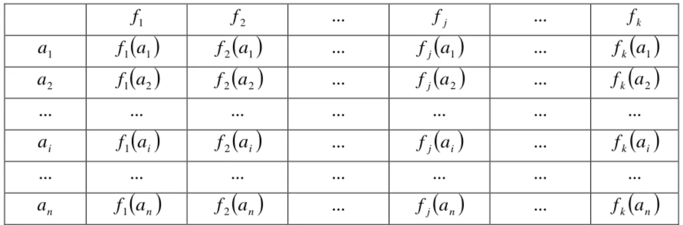
A general multicriteria decision problem can be defined through table 1 where the set of alternatives (i.e. a possible decision or an item to evaluate) is represented by
A
a
1,...,
a
n
, and the set of criteria (i.e. attributes associated to each alternative that makes it possible to evaluate the alternatives and to find the most suitable ones) byF
f
1,...,
f
n
. The evaluation value (i.e. number associated to each alternative with respect to criterion) of alternativea
i with the respect to the j-th criterion can be defined by fj(ai). The main goal ofDM is to find the alternative which best optimizes/trades-off all the criteria. The solution of multicriteria decision problem depends not only on the alternatives' values, but it is also mostly affected by different criteria weights assigned by different DMs.
Table 1. MCDA table 1
f
f
2 … fj …f
k 1a
f1
a1 f2
a1 … fj
a1 …f
k
a
1 2a
f
1
a
2f
2
a
2 … fj
a2 …f
k
a
2 … … … … ia
f
1
a
if
2
a
i …f
j
a
i …f
k
a
i … … … … na
f
1
a
nf
2
a
n … fj
an …f
k
a
n Detailed method histories, descriptions, properties and limitations together with available tools are presented in the following subchapters.3.2 Ranking
Ranking is the process of putting a set of alternatives in order from the most desirable to the least desirable based on values of multiple criteria. Since usually not all criteria are equally important, criteria weights are used to express the criteria importance.
AHP
The Analytic Hierarchy Process (AHP) is one of the most popular mathematical method applied for MCDA. It was developed by Thomas L. Saaty in the 1970s and it can be defined as a structured technique for organizing and analysing complex decisions [20]. Initially developed for contingency planning [21], the method can be used for solving decision making problems in almost any type of subject.
The main objective of the AHP method is to get ranking of a finite set of alternatives in terms of a finite number of decision criteria. It is based on establishing preferences between criteria and alternatives using pairwise comparisons. The most suitable alternative for a DM is always the best ranked.
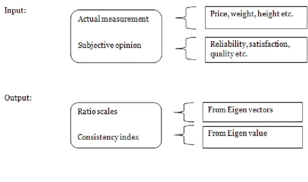
As shown on the Figure 2 it is possible to use as input to AHP method actual measurements like height, weight and price or use subjective opinions like reliability, satisfaction and quality. The output of the AHP method, as shown on the Figure 2 , are the ratio scales that describe DMs preference in comparing two elements in decision making process using intensity of importance defined in table 3. The ratio scales are obtained from the Eigen vectors that are used to derive the priorities between compared elements.
Another output is consistency index (CI) obtained from the Eigen values that are used to derive priority vectors. Saaty proposed the consistency ratio to check the consistency of comparing two elements in decision making process. The consistency ratio (CR) is calculated by dividing the consistency index (CI) by the random consistency index (RI).
RI
CI
CR
(1)
Table 2. Random consistency index table (n represents the number of items compared in matrix)
The random consistency index is obtained from the table 2 with respect to number of elements compared in matrix that is defined in table 4. If the value of consistency ratio is smaller than 0.01, the inconsistency is acceptable. If the consistency ratio is greater than 0.01, DM needs to revise its subjective judgments. If the value equals to 0 then that means that the judgments are consistent.
The hierarchical structure of the AHP method is shown on the Figure 3. It consists of a goal at the top, criteria influencing the goal in the next level down, possibly subcriteria in levels below that and alternatives of choice at the bottom of the model. In the AHP method the independence among criteria, subcriteria or alternatives is assumed. If the decision problem assumes dependence among criteria, subcriteria or alternatives, the ANP method is more appropriate and will be further discussed.
n 1 2 3 4 5 6 7 8 9 10
RI 0 0 0.58 0.9 1.12 1.24 1.32 1.41 1.45 1.49
AHP involves ten steps, as follows:
1. Define the main goal of your decision problem.
2. Structure elements of the decision problem in groups of criteria, sub-criteria, alternatives.
3. Construct a pairwise matrix as shown by the example in table 4.
a. All criteria are compared one-to-one with the other criteria using the Saaty scale as proposed in table 3, e.g. if something is considered twice as important as something else, a weight of 2 is given in the matrix for that relation. Apply the same comparison procedure for comparing sub-criteria and alternatives.
4. Normalizing matrix weights.
a. Each weight is divided by the sum of all weights in each matrix column. 5. Deriving a priority vector, i.e. the resulting relative weights
a. The sum of each row of normalized weights gives a priority vector. 6. Calculating a maximum Eigen value vector.
a. The product of the pairwise matrix (step 3) and the priority vector (step 5). 7. Calculating the consistency index.
a. The sum of the values in a maximum Eigen value vector is subtracted by the number that represents the size of the comparison matrix (e.g. the size is equal to 3 if there are 3 alternatives) and divided by the size of the comparison matrix minus 1.
8. Calculating the consistency ratio.
a. The consistency ratio is calculated by dividing the consistency index (CI) by the random consistency index. A consistency check is made to see if the ratio is smaller than 0.1. If the value of consistency ratio is smaller or equal to 0.1, the inconsistency is acceptable. If the inconsistency ratio is greater than 0.1, there is need to revise the subjective judgment.
9. Evaluate the criteria and alternatives with respect to the weighting. 10. Get ranking.
The pairwise comparison judgments used in the AHP pairwise comparison matrix are defined as shown in the Fundamental Scale of the AHP in the table below.
Table 3. The fundamental scale of AHP
Intensity of importance
Definition Explanation
1 Equal importance Two elements contribute
equally to the objective
3 Moderate importance Experience and judgment
slightly favor one element over another
5 Strong importance Experience and judgment
strongly favor one element over another
7 Very strong importance An activity is favored very strongly over another
9 Absolute importance The evidence favoring one
activity over another is of the highest possible order of affirmation
2,4,6,8 Used to express intermediate values
Decimals 1.1, 1.2, 1.3, …1.9 For comparing elements
that are very close Rational numbers Ratios arising from the scale
above that may be greater than 9
Use these ratios to complete the matrix if consistency were to be forced based on an initial set of n numerical values Reciprocals If element i has one of the
above nonzero numbers assigned to it when compared with element j, then j has the reciprocal value when compared with i
If the judgment is k in the (i, j) position in matrix A, then the judgment
1/k must be entered in the
inverse position (j, i).
To compare n elements in pairs construct an n x n pairwise comparison matrix A of judgments expressing dominance. For each pair choose the smaller element that serves as the unit and the judgment that expresses how many times more is the dominant element. Reciprocal positions in the matrix are inverses, that is aij 1 /aji.
The AHP process is here described in details. The goal represents the parent node of the criteria and they comprise one of the comparison groups. The criteria will be pairwise compared with respect to the goal. The pairwise comparison judgments are made using
table
3
and the judgments are arranged in a matrix, called the pairwise comparison matrix.Considering an example comprising of 4 criteria, the numbers in the cells in an AHP matrix as shown on
table 4
, by convention, indicate the dominance of the row element over the column element. In the AHP pairwise comparison matrix intable 4
the (Criteria_2, Criteria_3) cell has a judgment of 3 in it, meaning Criteria_2 is moderately important than Criteria_3. So logically this means Criteria_3 has to be 1/3 as important as Criteria_2. Thus, 1/3 needs to be entered in the (Criteria_3, Criteria_2) cell. The diagonal elements are always 1, because an element equals itself in importance.There will be 6 judgments required for these 4 elements. If the number of elements is n then the number of judgments is n(n-1)/2 to do the complete set of judgments.
Table 4. The AHP pairwise comparison matrix
Criteria_1 Criteria_2 Criteria_3 Criteria_4
Criteria_1 1 1/4 1/3 1/2
Criteria_2 4 1 3 3/2
Criteria_3 3 1/3 1 1/3
Criteria_4 2 2/3 3 1
The priorities of an AHP pairwise comparison matrix are obtained by solving the principal Eigen vector of the matrix. The mathematical equation for the principal Eigen vector w and principal Eigen value
max of a matrix A is presented by equation (2). It saysthat if a matrix A times a vector w equals a constant (maxis a constant) times the same vector, that vector is an Eigen vector of the matrix. Matrices have more than one Eigen vector; the principal Eigen vector which is associated with the principal Eigen value max (that is, the largest Eigen value) of A is the solution vector used for an AHP pairwise comparison matrix. The Eigen vector of the matrix shown in table 4 is depicted in table 5 and the most important criteria with the respect to goal is Criteria_2.
w
Table 5. Eigen vector for matrix shown in table 4 Criteria Priorities Criteria_1 0.0986 Criteria_2 0.425 Criteria_3 0.1686 Criteria_4 0.3077 Total 1.000
Perron's Theorem [22] shows that for a matrix of positive entries, there exists a largest real Eigen vector and its Eigen vector has positive entries. This is an important theorem that supports the use of the Eigen vector solution in AHP theory to obtain priorities from a pairwise comparison matrix. The book [23] gives more details about the mathematics background of the pairwise comparison matrix.
The AHP uses a data structure called a Super Matrix that contains priorities of the children from a comparison group of children and priorities of the parent from the comparison group of the parent. The name Super Matrix is used for this matrix because it is made up of column vectors of priorities, each of which was obtained from a matrix. So in a way it is a matrix of matrices.
There are three Super Matrices:
1) The unweighted Super Matrix contains the derived priorities obtained from the pairwise comparison results.
2) The weighted Super Matrix, weighted by the importance of clusters, is important only in network models [24], and will be discussed in the next subsection. The weighted Super Matrix is the same as the unweighted Super Matrix for hierarchy model. In the weighted Super Matrix all columns must sum to zero.
3) The limit Super Matrix is the final version of the Super Matrix obtained by raising the weighted Super Matrix to powers until all columns are the same (i.e. until it converges).
The simple way to get the ranking of alternatives for a hierarchy is to multiply the priority of each element in the hierarchy (derived through pairwise comparisons) by the weight of its parent element and sum the bottom level priorities of the alternatives to get the final ranking.
However, the solution may also be obtained using a Super Matrix. The weighted Super Matrix is raised to powers until it converges to the limit Super Matrix which contains the final results, the priorities for the alternatives, as well as the overall priorities for all the other elements in the model.
Since the AHP method is based on establishing preferences between criteria and alternatives using pairwise comparisons, it only supports quantitative values as input values to matrices (i.e. qualitative values, handling missing data, etc. is not supported by this method).
One of the advantages using the AHP method is that it allows decomposing a large problem into its constituent parts using the hierarchical structure. When the problem is presented with the hierarchical structure it becomes very easy to explain to other people. Since AHP is one of the first methods used in multi criteria decision analysis, there are a lot of tools which implement this method. It is also possible to create its own Excel sheet implementing AHP method which can then be used for decision problems with different number of criteria.
On the other side, the disadvantage of using AHP method may be a limited number of criteria. Since it is necessary to perform n(n-1)/2 pairwise comparisons it is recommended to use not more than 10 criteria. DMs are often not used to give a pairwise comparisons between items (i.e. it may be difficult to decide if one alternative is strongly or more strongly preferable than another alternative). They are more used to give either a sorting or ranking based on the importance. If the consistency index is too high, it may be a problem to explain to people to make another pairwise comparisons and reconsider their inputs. This method suffers from the rank reversal problem (i.e. the ranking can be reversed when a new alternative is introduced).
ANP
The Analytic Network Process (ANP) method represents a generalization of the Analytic Hierarchy Process (AHP). It was developed in 1996. by Thomas L. Saaty and has been applied in many research papers such as research on evaluation index system of mixed-model assembly line [25], university-industry alliance partner selection method [26], partner selection method for supply chain virtual enterprises [27], etc.
The main objective of the ANP method is to get ranking of a finite set of alternatives in terms of a finite number of decision criteria. It is based on establishing preferences between criteria and alternatives using pairwise comparisons. The most suitable alternative for a DM is always the best ranked.
The structure of ANP is shown on Figure 4. It consists of 4 clusters and 7 nodes. The decision nodes are organized in a network of clusters with links between the nodes going in either direction or both directions. The first cluster consists of Goal, the second cluster of Criteria 1 and 2, the third cluster of Criteria 3 and 4, and the fourth cluster of Alternative 1 and 2. As shown, in ANP nodes might be grouped in cluster whereas in AHP this is not possible. Thus, beside priorities in the comparison of one node to a set of other nodes, it is also possible to define cluster priorities with respect to the goal. Matrix is used to represent the network of ANP. This matrix is composed by listing all nodes horizontally and vertically. The connection and weight between one node (columns-header) to another node (row-header) of the network is presented entering values from the table 3. After populating all rows and columns, this matrix becomes so called Super Matrix consists of values expressing relative importance of one node/cluster to other node/cluster.
The pairwise comparison of nodes or clusters to each other‟s and the calculation of local priorities are the same as in AHP method. After calculating the Eigen vector of the pairwise comparison matrix we get the local priorities arranged as column vectors in the super matrix. After all comparisons are completed we get an unweighted Super Matrix of the network model. The matrix then needs to be normalized and we get resulting weighted Super Matrix. The whole model is synthesized by calculating the weighted Super Matrix, taken to the power of k + 1 until it converges (in this case all columns are the same), where k is an arbitrary number. The weighted Super Matrix is called the Limit Matrix. The final result is ranking of the alternatives in network model.
Difference in structure between AHP and ANP is shown on Figure 5. A hierarchy in AHP is a network too, but a special kind of network with a goal cluster from which all the arrows lead away, and a sink cluster (the alternatives) that all the arrows lead into. Links go only downward in a hierarchy. A typical network has neither sinks nor sources; and the links can go in any direction. A network can more faithfully represent the relative world we really live in. Let‟s consider an example of buying a car. One does not buy a car by determining in the abstract the importance of the criteria before going shopping and looking at a few cars. The available cars determine how important the criteria are. And when new cars are added to those being considered, the importance of the criteria may change. Thus, ANP reflects the way how we make decisions where the importance of criteria can change with the available alternatives.
Since the ANP method is based on establishing preferences between criteria and alternatives using pairwise comparisons, it only supports quantitative values in range from 1 to 9 as input values (i.e. qualitative values, handling missing data, etc. is not supported by this method).
One of the advantages using ANP method is introduction of clusters and links between the elements going in either one direction or both directions. Thus, it is possible to deal with more complicated problems. Also, we can obtain much deeper understanding of a decision problem and interconnections between elements in the structure.
On the other side, the disadvantage of using ANP method may be a limited number of criteria and alternatives. Since it is necessary to perform n(n-1)/2 pairwise comparisons it is recommended to use not more than 5 criteria and alternatives in a cluster. People are often not used to give a pairwise comparison between items. They are more used to give either a sorting or ranking based on the importance. If the consistency index is too high, it may be a problem to explain to people to make another pairwise comparison and reconsider their inputs. Due to feedback loops and interconnections it may be very difficult to create own implementation of ANP in Excel spreadsheet, so it is necessary to obtain a specific software. This method suffers from the rank reversal problem (the ranking can be reversed when a new alternative is introduced).
TOPSIS
TOPSIS is an acronym for Technique for Order Preference by Similarity to Ideal Solution. It is multiple-criteria decision analysis method proposed by Hwang and Yoon in 1981. It is used for ranking the alternatives with a finite number of criteria.
The method is not limited to a specific field and so far has been applied in supply chain management and logistics [28], [29], business and marketing management [30], energy management [31], chemical engineering [32] etc.
TOPSIS method is getting into account the distance of alternatives from the positive-ideal and negative-positive-ideal solution.
Paper [19] provides a method explanation and it was a source for the following formulas. It has five steps. The first step after creating the decision matrix is the normalization of the input data. The construction of the normalized decision matrix is done using the formula
m i ij ij ijx
x
r
1 2for i=1,…,m; j=1,…,n;
(3)
where xij are original and rij are normalized values.
After that the weighted normalized decision matrix is created in the second step, taking into account the criteria importance with the formula vij wjrij where wj is the weight of j criterion.
The positive and negative ideal solutions are determined in the step 3. Positive ideal solution is given by the following formula
}
,...,
,...,
,
{
}
,...
2
,
1
|
)
'
|
min
(
),
|
max
{(
* * * 2 * 1 * * n j ij i ij iv
v
v
v
A
m
i
J
j
v
J
j
v
A
(4)
The negative ideal solution is
} cos | ,..., 2 , 1 { ' } | ,..., 2 , 1 { } ' ,..., ' ,..., ' , ' { ' } ,... 2 , 1 | ) ' | max ( ), | min {( ' 2 1 criteria t with associated j n j J where criteria benefit with associated j n j J where v v v v A m i J j v J j v A n j ij i ij i
(5)
In step 4 the separation from the positive and the separation from the negative ideal alternative are calculated.The separation from the positive ideal solution is calculated by formula m i v v S n i j ij i ( ) 1,2,..., 1 2 * *
(6)
and the separation from the negative ideal solution is given by formulam
i
v
v
S
n i j ij i'
(
'
)
1
,
2
,...,
1 2
(7)
In the fifth step the closeness coefficients are calculated.
' 0 1 ,..., 2 , 1 , 1 0 , ' ' * * * * * * A A if c A A if c m i c S S S c i i i i i i i i i (8)
The alternatives are ranked according to the descending order of the closeness coefficient values, so the higher the value the better the solution.
TOPSIS method supports quantitative values and it is relatively simple to use and implement. Therefore the method is widely used in numerous real-life problems. There are also multiple tools that support this method.
The negative side of the method is that it does not support uncertain or missing values. Like most of the MCDA methods it could suffer from rank reversal problem.
VIKOR
VIKOR is a method used in multicriteria decision analysis developed in 1998. by Serafim Opricovic. It has been applied in many areas such as neural network [33], multi-criteria decision making problems under intuitionistic environment [34], suppliers selection [35], etc.
The main objective of the VIKOR method is to evaluate several possible alternatives according to multiple conflicting criteria and rank them from the worst to the best one. The most suitable alternative for DM is always the best ranked.
It is based on ranking and selecting from a set of alternatives. The positive and negative ideal solutions are defined. The positive ideal solution is the alternative with the highest ranked value in terms of benefit, and the lowest ranked value in terms of cost. The negative
ideal solution is the alternative with the lowest ranked value in terms of benefit, and the highest ranked value in terms of cost.
The procedure of VIKOR method consists of several steps:
1. First we need to compute the best and the worst value of each criteria.
Suppose we have m alternatives, and n criteria. Various j alternatives are denoted as A(1), A(2), ... , A(j).Letfij presents the value of the ith criterion function for the alternative A(j). The best value for all n criteria functions is denoted as
fi* and presents the positive ideal solution for the ith criterion. The worst value
for all n criteria functions is denoted as fi- and presents the negative ideal solution for the ith criterion. If ith criterion function represents a benefit then
the following equations can be obtained, as defined in [36]:
*
max
i i ijf
=
f
f
i-=
min
if
ij(9)
If ith criterion function represents a cost then the following equations can beobtained, as defined in [36]:
*
min
i i ijf
=
f
f
i-=
max
if
ij(10)
2. For each alternative compute the ideal value Sj (or utility measure) and negative value Rj (or regret measure) using the following equations, as defined in [36]:
n i i i ij i i j f f f f S 1 * *
i i ij i i i j f f f f R * *max
where j = 1 , ..., m andi = 1, ..., n
(11)
Wi are the weights of criteria expressing DM‟s preferences and may be
assigned using the AHP method.
3. For each alternative compute the synergy value Qj using the following equations, as defined in [36]:
*
* * * 1 R R R R v S S S S v Qj j j * min max j j j j S S R- R = = * max min j j j j S S R R -= = where j = 1, ...,m and i = 1, ..., n
(12)
v represents the weight for the strategy of maximum group utility and can
take any value from 0 to 1. It is usually set to value 0.5.
4. The final step consists of ranking the alternatives by measured values S, R and Q in decreasing order and then proposing a compromise solution consisted of the alternative A(1) which represents the best ranked solution by the measure Q (minimum) [36].
When the compromised solution is proposed, two conditions must be satisfied:
-
a) Acceptable advantage – (A(2) denotes the second best ranked alternative)
DQ A Q A Q 2 1 where 1 1 DQ m = -(13)
b) Acceptable stability in decision making - the proposed alternative A(1) must also be best ranked by S and/or R.
If one of the conditions mentioned above is not satisfied, alternative solutions are:
a) Alternatives A(1) and A(2) if the condition b) is not satisfied.
b) Alternatives A(1), A(2), ..., A(m) if the condition a) is not satisfied. A(m) is determined by the relation
(
(M))
( )
(1)Q A - Q A <DQfor maximum M.
Compared to AHP method, in VIKOR method it is not necessary to perform consistency test, as discussed in AHP chapter. This method supports only quantitative values and it is relatively simple to use and implement.
The VIKOR method has a significant advantage over the other ideal point method, such as TOPSIS method, because the “VIKOR algorithm can order directly without considering that the best solution is closer to the ideal point or more farther to the worst ideal point” [37]. On the other side, there is no available tool developed that implement this method. VIKOR is not able to handle incomplete and uncertain information. This method suffers from the rank reversal problem (i.e. the ranking can be reversed when a new alternative is introduced).
PROMETHEE I AND II
PROMETHEE is an acronym for Preference Ranking Organization Method for Enrichment Evaluations. It was developed in the 1980s and applied in many areas such as automotive sector [38], web service selection [39], exploration strategies for rescue robots [40], suppliers evaluation [41], etc.
It is based on building an outranking on the set of alternatives in which the main objective is to find the alternative that is the most suitable for DM. Outranking methods are based on a more familiar way of thinking. Instead of trying to define what is good and what is bad, it is usually much easier to compare one solution to another. That is the underlying principle of outranking methods.
There are different types of PROMETHEE methods (and their extensions). The family of PROMETHEE methods is presented in table 6.
Table 6. Family of PROMETHEE methods
Name of method Short description
PROMETHEE I Used for a partial ranking – considers
only dominant characteristics of one alternative over other. Based on the positive and negative flows.
PROMETHEE II Used for a complete ranking –
considers both dominant and outranked characteristics of one alternative over other. Based on the net flow.
PROMETHEE III extension Extension to PROMETHEE II which is based on interval ranking of alternatives [44].
PROMETHEE IV extension Extension to PROMETHEE II which includes the infinite set of actions (continuous set of possible alternatives), but was never further developed nor applied [42].
PROMETHEE V extension Extension to PROMETHEE II that
supports the optimization under constraints [43].
PROMETHEE VI extension Extension to PROMETHEE II which includes the sensitivity analysis procedure into decision making process [44].
The PROMETHEE I and II methods consist of several steps that are subsequently described. In the first step a preference function has to be associated with each criterion in
order to reflect the perception of the criterion scale by the DM. Usually the preference function Pj
ai,ak
is a non-decreasing function of the difference fj
ai fj
ak between theevaluations of two alternatives
a
i anda
k. Several typical shapes of preference functions are proposed in the literature [45], and indications are given on the way to select appropriate functions for different types of criteria. The value of Pj
ai,ak
is a number between 0 and 1. It corresponds to the degree of preference that the DM express fora
i overa
k according tocriterion fj. Value 0 corresponds to no preference at all while 1 corresponds to a full preference.
In a second step the DM assesses numerical weights to the criteria to reflect the priorities: more important criteria receive larger weights. We note wj the weight of criterion
j
f and we assume that the weights are normalized (sum of all weights are equal to one). A
multicriteria pairwise preference index is then computed as a weighted average of the preference functions:
k j k i j j k ia
P
a
a
a
1,
,
(14)
Three preference flows are then computed in order to globally evaluate each alternative with respect to all other ones. The positive flow is a measure of the strength of an alternative
i
a
with respect to the other ones, the negative flow is a measure of the weakness of analternative
a
i with respect to the other ones. Finally the net flow is the balance between the two first ones. Obviously the best alternative should have a high positive value (close to 1) and a low negative value (close to 0), and thus a high positive balance value.PROMETHEE I ranking is obtained by looking at the positive flow value and negative flow value. It is a partial ranking as the two flows usually give a different ranking of the alternatives because they synthesize the pairwise comparisons of the alternatives in two different ways. A traditional way to present PROMETHEE 1 is via a network representation where arrows indicate preferences. However that representation doesn‟t give any visual information about the differences between the flow values. It is for instance difficult to appreciate how the ranking would be influenced by small changes in the weighting of the criteria.
PROMETHEE II final ranking is obtained by net flow values. All alternatives are compared but the differences between the positive and entering flows are lost, leading to a possibly less robust ranking.
These methods are able to handle only quantitative and missing values in information table. When the missing value is encountered, the PROMETHEE I and II methods perform all the pairwise comparisons and the resulting preference degree is set to zero as if both alternatives had equal evaluations on that criterion.
The advantages of using PROMETHEE II methods are listed as follows. The PROMETHEE 2 method classifies alternatives which are difficult to be compared because of a trade-off relation of evaluation standards as non-comparable alternatives. It is not necessary to perform a pairwise comparisons again when comparative alternatives are added or deleted. [46]
On the other side, these methods suffer from the rank reversal problem (the ranking can be reversed when a new alternative is introduced).
EVIDENTIAL REASONING
Evidential reasoning approach is a MCDA method that is applied in many areas such as object recognition system [47], remote sensing images [48], evaluating students learning ability [49], fault diagnosis [50], etc.
The main objective of the method is ranking the alternatives with a finite number of criteria.
This method is also able to address uncertainties such as incomplete information using belief structure based on Dempster-Shafer theory of evidence [51]. The missing data in incomplete decision matrix are denoted by “*“. Dempster-Shafer theory provides methodology for solving incomplete decision matrix. It is necessary to ensure that the values in decision matrix are qualitative. If they are quantitative, the direct application of this approach may lead to large errors.
For example, when assessing the quality of specific hardware-software component for our system, we can have five evaluation grades:
1 2 3 4 5
, , , , , , , , Worst Poor H H H H H H Average Good Excellent (15)
Suppose we have G alternativesAj
j1,...,G
and we need to evaluate them with respectto T criteria C ii
1,...,T
. The assessment of a criterion C on an alternative 1 A where 1 n,1presents the degree of belief that the criterion C1 is assessed to the evaluation gradeHn is
presented using the belief structure:
1 1
1,1, 1
, 2,1, 2
, 3,1, 3
, 4,1, 4
, 5,1, 5
S C A H H H H H
(16)
The value of n,1 is always between 0 and 1 and the sum of all degrees of belief ( 1,1, 2,1, 3,1, 4,1, 5,1in our case) must not be larger than 1. If the sum of all degrees of belief is equal to 1 we have a complete distributed assessment, otherwise we have an incomplete assessment.For example, the distributed assessment result of the quality of specific hardware-software component for criterionC1with the respect to alternativeA1for our system could be:
1 1
Excellent, 40% , Good, 20% , Average, 20% , Poor, 0% , Worst,0%
S C A
(17)
The above can be read as follows: We have 40% of belief degree that the quality of specific hardware-software component for our system is excellent, 20% that the quality is good or average and 0% of belief degree that the quality is poor or worst.
For each criterion we can define an extended decision matrix S C A
1
1
which consists of T criteria C ii
1,...,T
, G alternatives Aj
j1,...,G
and N evaluation grades
1,..., N
n H n :
i j
n, n i,
j
S C A H A n1,...,N i1,...,M j1,...,K (18) The main goal of Evidential reasoning algorithm is to aggregate belief degrees based on the Dempster-Shafer theory. Thus, in Evidential reasoning approach it is not necessary to aggregate average scores and in this way this method is different from other MCDA methods.Suppose we have the following two complete criterion assessments and we need to aggregate them to generate a combined assessment.
1 1
1,1, 1
, 2,1, 2
, 3,1, 3
, 4,1, 4
, 5,1, 5
S C A H H H H H
2 1
1,2, 1
, 2,2, 2
, 3,2, 3
, 4,2, 4
, 5,2, 5
S C A H H H H H (19)The next step is to define a basic probability mass mn j,
j1, 2
and the remaining belief
, 1, 2 H j
m j for criterion j (with weighti) unassigned to any of the Hn
n1,..., N
as follows (equations are obtained from [52]):
,1 1 ,1 1,...,5 n n m n 5 ,1 1 ,1 1 1 1 1 H n n m
,2 2 ,2 1,...,5 n n m n 5 ,2 2 ,2 2 1 1 1 H n n m
(20)To generate a combined probability massesm nn
1,...,5
and m we need to use the HEvidential Reasoning algorithm to aggregate the basic probability masses as follows (equations are obtained from [52]):
,1 ,2 ,1 ,2 ,1 ,2
n n n H n n H m k m m m m m m
n1,...,5
,1 ,2
H H H m k m m 1 5 5 ,1 ,2 1 1 1 t n t n k m m
(21)We can aggregate the combined probability masses for all other criteria at the same way. Because we have only two assessments, the combined degrees of belief n
n1,...,5
, as defined in [52], are generated by:1 n n H m m
n1,...,5
(22)The final assessment for the alternativeA can be defined as follows: 1
1
1, 1
, 2, 2
,
3, 3
, 4, 4
,
5, 5
S A H H H H H
(23)
An average score for alternative
A1can be defined as follows:
1 5
1 i i i u A u H
(24)
Where u H is the utility of the i-th evaluation grade
i H . By applying the equation (24) iit is possible to obtain the utility interval for all decision alternatives of the problem with incomplete decision matrix and get the final ranking of alternatives.
The biggest advantage is the possibility of handling qualitative and missing data using belief matrix structure. The evidential reasoning approach is implemented in Intelligent Decision System software (IDS) which is fully functional without any limits and is available for free.
The disadvantage of the method is that it is implemented in only one tool (IDS) which has the limitation on the size of the decision problem. It cannot handle decision problems with more than 50 alternatives and 50 criteria. This method is too complex to be manually implemented.
3.3 Classification
Classification is the process of assigning alternatives to a set of predefined classes or categories. Depending on the method used classes could be defined using training examples or manually by the DM.
RSA
RSA is an acronym for Rough Sets Approach. It is a specific type of multi-criteria decision analysis method based on a classification. It was introduced by Pawlak [53]. It is used in many areas such as breast cancer classification [54], approximation of sensor signals [55], measuring information granules [56], cognitive radio networks [57], etc.
The main objective of this method is extraction of the classification rules from a set of already classified examples. Extracted rules can be used to make partition of new data sets and they are presented in the form similar to human language as “if…then…” sentences.
The following description of the rough set approach is obtained from [58]. This method concerns with an experience that is recorded in a structure called an information system. The information system may contain various types of information (e.g. events, observation, states, etc.) in terms of their criteria (e.g. variables, characteristics, symptoms, etc.). There are two groups of criteria. The first group is called “condition criteria” and it takes into account results of some measurements or data from observations. The second group of criteria is called “decision criteria” and it concerns with the expert‟s decisions. The most