J
Ö N K Ö P I N GI
N T E R N A T I O N A LB
U S I N E S SS
C H O O L JÖNKÖPING UNIVERSITYT h e v o l a t i l i t y r a c e i n C o m m o d i t i e s
A s t u d y o f t h e o p t i m a l h e d g e r a t i o i n C o p p e r ,
G o l d , O i l a n d C o t t o n
Master thesisAuthors: Haglund, Fredrik Svensson, Johan Tutor: Wramsby, Gunnar Jönköping 27th May 2005
Master thesis in Business Administration
Title: The volatility race in commodities - A study of the optimal hedge ratio in Copper, Gold, Oil and Cotton
Authors: Fredrik Haglund and Johan Svensson Tutor: Gunnar Wramsby
Date: 27th May 2005
Subject terms: commodities, hedging, optimal hedge ratio, futures, Oil, Copper, Cotton, Gold
Abstract
IntroductionCompanies that are dependent on different commodities as input or output are ex-posed to price risk in these commodities. The price changes can be expressed as vola-tility and higher volavola-tility results in higher risk. Hedging the commodity contracts with futures can offset this risk. One of the most important questions in this field is to what extent the risk exposure should be hedged with futures contract, i.e. the op-timal hedge ratio.
Purpose
The study aims to conduct an analysis of the variance in different commodities con-tracts and provide evidence of the optimal hedge ratio in the respective commodities. Method
We used a quantitative study with daily spot and futures price changes of Copper, Gold, Cotton and Oil. We investigated the 6-month hedging behaviour where time-series were created for the period January-June each year during 2001-2004. We used a simple linear regression of the futures and spot price changes and a minimum vari-ance model in order to calculate the optimal hedge ratio.
Conclusion
Companies that are dependent on Copper, Gold, Cotton and Oil can significantly reduce the risk by engaging in futures contracts. The optimal hedge ratio for Copper is (96%), Gold (52%), Cotton (96%) and Oil (88%). By applying the optimal hedge ra-tio, a company may reduce their risk exposure up to 90% compared to an unhedged position.
Table of Contents
1
Introduction ... 4
1.1 Background ... 4 1.2 Problem discussion ... 5 1.3 Research questions ... 5 1.4 Purpose ... 5 1.5 Delimitations... 62
Frame of Reference ... 7
2.1 Futures Markets ... 7 2.1.1 Basis Risk... 72.1.2 Futures Pricing and Contracts ... 8
2.2 Hedging and Optimal Hedge Ratio ... 8
2.2.1 Optimal Hedge Ratio for Commodities ... 9
2.3 General Statistical tests ... 11
2.3.1 Test for Stationary Time Series ... 11
2.3.2 Test for Normality ... 12
2.3.3 Test for Autocorrelation... 13
2.3.4 Test for heteroscedasticity ... 14
2.4 The Optimal Hedge Ratio and Risk Reduction statistics ... 14
2.4.1 The Minimum Variance Hedge Ratio ... 14
2.4.2 Simple Linear Regression Analysis ... 15
2.4.3 Risk Reduction ... 16
3
Methodology... 17
3.1 Applied Method ... 17
3.2 Data collection... 17
3.2.1 Data ... 18
4
Empirical findings and Analysis... 20
4.1 General statistic ... 20
4.1.1 Copper... 20
4.1.2 Gold ... 21
4.1.3 Cotton... 22
4.1.4 Oil ... 23
4.2 Optimal Hedge Ratio and Risk Reduction ... 24
4.2.1 Copper... 24 4.2.2 Gold ... 26 4.2.3 Cotton... 27 4.2.4 Oil ... 28
5
Conclusion ... 31
6
Final discussion ... 32
6.1 Methodology criticism... 346.2 Further research recommendations... 34
Tables
Table 1 Copper statistics for June contracts 2001-2004 ... 21
Table 2 Gold statistics for June contracts 2001-2004... 22
Table 3 Cotton #2 statistic for June contracts 2001-2004 ... 22
Table 4 Oil Light Crude statistic for June contracts 2001-2004... 23
Table 5 Copper OHR and Risk Reduction ... 25
Table 6 Gold OHR and Risk Reduction... 26
Table 7 Cotton OHR and Risk Reduction ... 27
Table 8 Oil Light Crude OHR and Risk reduction... 28
Appendices
Appendix 1 Copper price level time-series data... 39Appendix 2 Gold price level time-series data ... 41
Appendix 3 Cotton price level time-series data... 43
1 Introduction
1.1 Background
Companies that are dealing with commodities either as input for production or as output are vulnerable to price changes in these commodities. Surging commodity prices will be painful for companies that use these commodities in their production process, with increasing raw material costs and decreasing profit margins as a result. On the other hand, companies in for example the mining industry gain from an in-crease in the market price of for example Gold or Copper. Naturally, companies that are dependent on a number of commodities either as an input or output are exposed to a number of risks when the commodity prices move in an undesired direction, e.g. increased and unpredictable raw material costs, reduced profit margins and falling share prices (Cameron, 2002; Leuthold & Tzang, 1990; Uptigrove, 2004)
It is not only the oil price that has experienced a significant increase during the last years but also all the metal prices have seen a similar development. As an example, the price of copper has increased 179 percent in the last two years (Commodity Price Index, 2005). These substantial price fluctuations affect not only single companies but also industries and even countries, since some countries are heavily dependent on its commodity export or import (Satyanarayan, Thigpen & Varangis, 1994).
The market for commodities has a long history, agricultural futures contracts have been trading since the 1800s and metal futures contracts since the 1930s (Siegel & Siegel, 1990). Companies as well as speculators use the market extensively. The mar-ket price (spot price) of a commodity, changes accordingly to supply and demand in the same way as the price of a share. Commodities are traded in contracts and differ in amount and time from one commodity to another. The same thing is true for the futures. The futures can be used both for speculation and hedging (Siegel & Siegel, 1990). Several researches suggest that hedging is an effective way to reduce risk expo-sure. Although most agree, numerous studies highlight the implication by choosing the amount to hedge i.e. the hedge ratio (Baillie & Myers, 1991; Ederington, 1979; Satyanarayan, et al, 1994).
In a study by Byström (2000) the hedging performance of Electricity Futures on the Nordic Power Exchange (Nord Pool) were examined. Byström (2000) presents em-pirical results that indicated of gains from hedging. Baillie and Myers (1991) ducted a study where six commodity contracts were examined over two futures con-tracts periods. The authors calculated the optimal hedge ratio in the six commodities. The results in this study indicated that different hedge ratios should be applied to dif-ferent commodities. Satyanarayan et al. (1994) investigated the hedging performance of different cotton futures contracts with four different hedge ratios and compared the risk, return and risk reduction in the different cotton futures. The authors con-cluded that the applied hedging techniques reduced risk in almost all cases. Moreover, Fackler and McNew (1991), Leuthold and Tzang (1990) have also studied hedge ratios in different commodity contracts, but found contradictionary results compared to previous studies, which makes the topic relevant for further studies.
The results from these studies are not only of academic relevance but also of practice importance. Companies that need commodities in their production could have a lot to gain from using futures contracts to hedge their input. A study that reveals the op-timal hedge ratio for a particular commodity would thereby be of significant interest in a business perspective.
1.2 Problem
discussion
All companies that are dependent on commodities are affected by the price changes in the commodities. The price changes can be expressed as volatility and higher vola-tility results in higher risk. Hedging the commodity contracts with futures can offset this risk. To be able to explain how hedging is actually performed we need to intro-duce a statistical term called variance, which is basically the difference between a set of data points around their mean value. The futures contract is purchased with the objective to minimize the variance between the future and spot price. When the fu-ture is minimizing the variance at the most, one is said to have an optimal hedge ratio (Siegel & Siegel, 1990).
Theories discuss the implications regarding the hedge ratio and numerous researchers have tried to solve this problem, without finding a standardized answer how to con-struct an optimal hedge ratio. Almost all previous studies in the academic area have been conducted in solely statistical manner without consideration to the business per-spective. It would hence be interesting to link the statistical tests results with a busi-ness perspective and try to give hedging suggestions to companies that are facing commodity risk exposure.
By investigate the variance in the historical spot and futures prices between 2001 and 2004 in four commodities; we aim to find evidence of the optimal hedge ratio in these commodity contracts. We will be able to evaluate the hedge ratios performance in the commodities and compare them to each other and thereby demonstrate how to con-struct the best optimal hedge ratio.
1.3 Research questions
• What is the variance in each respective commodity?
• What is the optimal hedge ratio to minimize the variance in each respective commodity?
• What is the risk reduction, when the optimal hedge ratio is applied in the re-spective commodities?
• How could a company gain from hedging the respective commodities?
1.4 Purpose
The study aims to conduct an analysis of the variance in different commodities con-tracts and provide evidence of the optimal hedge ratio in the respective commodities.
1.5 Delimitations
The aim of this thesis is not to forecast the future prices of the respective commodi-ties. Although a forecast of the optimal hedge ratio for the different commodities could partially be based on this study, it must be stated that a forecast of the future price fluctuations demands a more detailed analysis than just historical data as used in this thesis.
We make an assumption throughout this thesis that the objective of the hedger is to minimize risk regardless off the reduction trade off, e.g. the hedger is highly risk-averse.
We chose to analyse the futures contracts in our four commodities, excluding for-ward and option contracts. Firstly, the futures contracts are the most common method to hedge against commodity risk exposure on the different commodity ex-changes, and secondly, this thesis would be to vast if all the different derivative con-tracts were included.
When we discuss risk management, we exclude a foreign exchange risk perspective and focus exclusively on commodities. Thus, readers should keep in mind that this delimitation results in an incomplete illustration of the implications within risk man-agement.
2 Frame
of
Reference
The frame of reference chapter consists of four main parts. Firstly, we will present general theories about the futures market. Secondly, hedging theories and the optimal hedge ratio for the commodity market will be discussed. Thirdly, a number of gen-eral statistical tests that are important when analysing time-series data will be exam-ined. Lastly, the statistical tests for calculating the optimal hedge ratio and risk reduc-tion will be presented.
2.1 Futures
Markets
The futures market offers investors a number of investment opportunities, from re-ducing or eliminating risk to speculating on price movements in the spot market or to diversify the portfolio. Futures contracts represent agreements to take or make de-livery of some commodity at a later date. Futures are standardized so that size, deliv-ery procedures, expiration dates, and other terms are the same for all contracts. This standardisation allows futures to be traded on exchanges, which provides liquidity to market participants (Moy, 2000; Hull, 2003).
Futures have a number of useful applications. First, they can be used to hedge risk in the spot or cash market. By taking a position opposite to that position held in the spot market, it is possible to reduce or even eliminate risk. Second, because futures are essentially costless, they can be used to speculate on the future price of a com-modity. Third, because the futures contract is based on delivery of some asset or commodity in the spot market, there should be a relationship between the two prices. If these prices get out of line, an opportunity to arbitrage the difference be-tween the two prices will exist. And finally, futures can be used to adjust the risk of a portfolio (Moy, 2000; Hull, 2003).
2.1.1 Basis Risk
Basis is an important concept in understanding the pricing and risk of using futures contracts. Basis is the current spot market price of the commodity minus the price of the futures contract on that commodity. The basis can be either positive or negative. When the basis is positive, prices in the cash market are higher than the futures prices, also called backwardation. When the basis is negative, prices in the cash mar-ket are lower than the futures prices, also called contango (Siegel & Siegel, 1990). For example, the crude oil market is typically in backwardation whereas the Gold market typically is in contango (Cameron, 2002).
During the life of a futures contract, the basis will change. As the contract gets closer to expiration, the basis becomes smaller. At expiration, the basis of a contract will be zero because the futures price at expiration must equal the spot market price. Al-though the basis of a contract will equal zero at expiration, it can fluctuate during the life of the contract. The basis of a contract can widen or narrow. This type of risk is referred to as basis risk, which basically relates to the imperfect relationship between the future price and spot price at expiration. However, this is mostly an issue when
cross hedging is used. Cross hedging is a term to describe a hedge situation where an asset is hedged with the closest security that exists. For example, a share will be hedged with futures on the index that the underlying share is part of. Fortunately, there are futures contracts that exactly match most commodities today, which mean that the commodity that is supposed to be hedged has high correlation with the fu-tures contract and practically no basis risk needs to be accounted for (Moy, 2000; Hull, 2003; Siegel & Siegel 1990).
2.1.2 Futures Pricing and Contracts
The value of a futures contract is determined by the underlying commodity and the principle of arbitrage. Arbitrage occurs when it is possible for investors to earn a guaranteed profit without using any of their own money. This opportunity arises when the relationship between cash and futures prices gets out of line. In principle, the value of a futures contract should be equal to the current cash market price plus any cost of carrying the commodity. These costs include interest, storage, and insur-ance costs. When the prices of the two markets get out of line, arbitrageurs will drive the prices back to their equilibrium state by purchasing in the market where the price is too low and simultaneously selling in the market where the price is too high (Moy, 2000; Hull, 2003).
Four basic categories of futures contracts can be traded. The underlying asset or commodity can be a physical commodity, a foreign currency, an asset earning inter-est, or an index (Moy, 2000; Hull, 2003). We will only discuss futures contracts with an underlying physical commodity.
2.2 Hedging and Optimal Hedge Ratio
Hedging entails the reduction of risk by taking an opposite position in the futures market from the trader’s spot market position. There are different types of hedging strategies but all with the same intention to reduce risk. Basically there are two ways to use a futures contract for hedging. A company that knows that it is due to sell an asset at a particular time in the future can hedge by taking a short futures position. This is known as a short hedge. If the price of the asset goes down, the company makes a loss on the sale of the asset but makes a gain on the short futures position. If the price of the asset goes up, the company gains from the sale of the asset but takes a loss on the futures position. Similarly, a company that knows that it is due to buy an asset in the future can hedge by taking a long futures position, known as a long hedge. If the price of the asset rises, the futures position will profit and offset the company’s loss due to higher supply costs (Hull, 2003; Siegel & Siegel 1990).
The most common hedge does not make or take delivery, which mean that the fu-tures will not be executed. Instead, the seller (buyer) of the fufu-tures contract cancels his delivery commitment by buying (selling) a contract of the same futures prior to delivery (Ederington, 1979).
The hedge ratio is the ratio of the size of the position taken in futures contracts to the size of the exposure. Several types of hedge ratios can be produced depending on the type of risk that the hedger is concerned with. However, the following factors are usually important determinants of the hedge ratio:
1. Size of the spot or cash market position. 2. Size of the futures contract.
3. Sensitivity of spot price and futures price relative to some external factor.
The first two factors are quite obvious. The larger the size of the spot market posi-tions relative to the size of the futures contracts, the greater the number of contracts necessary to hedge the risk. The third factor adjusts the number of contracts for the different sensitivities of spot prices and futures prices. If the spot price changes 20 percent more when the futures price changes, the hedge ratio needs to be adjusted with that difference. More specifically, the hedge ratio needs to be 1.20, to reduce the risk. The hedger would thereby have to offset the risk with 1.20 futures contracts (Siegel & Siegel 1990).
2.2.1 Optimal Hedge Ratio for Commodities
In this section we present the academic research in the field of deriving an optimal hedge ratio for commodity contracts. The statistical model used in the different arti-cles will be presented since this is vital for comparison to our own study. In brief, the GARCH and the ordinary least square regression model are the two most common statistical methods. More importantly, the implication of the hedge ratio for the dif-ferent commodity contracts will be presented and the reduction in risk that this im-plies.
Risk evaluation has long been a focus for all financial institutions. Such evaluation cannot be done without measuring the volatility for asset returns. Engle (1982) devel-oped enhanced methods for conducting these kinds of evaluations. He discovered that the concept of autoregressive conditional heteroscedasticity (ARCH) accurately cap-tures the properties of many time-series and developed methods for statistical model-ling for time-varying volatility. Engle’s model has become an important tool for both researchers and financial analysts (Baillie and Myers, 1991; Bollerslev, 1986). Together with widely known CAPM and Black and Scholes, ARCH and its variety models are today used on a frequent basis when pricing derivatives and handling financial risks (Ekonomipriset, 2003).
It is crucial to understand the distribution of commodity cash and futures markets, when constructing optimal hedging strategies on the commodity markets. Baillie and Myers (1991) present a study, which investigates the distribution of commodity cash and futures prices of beef, coffee, corn, cotton, gold and soybeans. They apply the re-sults to estimate the optimal futures hedge. Early studies by Mandelbrot (1963) and Fama (1965) states that commodity price changes appear to be non-normal distrib-uted with volatile periods where variance changes over time.
In a study by Baillie and Myers (1991), the authors used a Generalized Autoregressive Conditional Heteroscedastic (GARCH) model, which was originally constructed by
Engle (1982) and enhanced by Bollerslev (1986). The advantage of a GARCH model is that convenient assumptions about the conditional density of commodity price changes can lead to a robust model that allows for time-dependent variances. The study concluded that the GARCH model was effective in describing the distribution of commodity cash and futures prices, and that it resulted in a natural description of time-varying optimal hedge ratios on commodity futures market (Baillie & Myers, 1991). However, it is important to mention that long-term contracts were used, up to two years (1985-1987). It seems reasonable that longer contracts also experience dif-ferences in variances, which would make a GARCH model suitable. Baillie and Myers (1991) also used an ordinary lest square (OLS) regression model (the OLS as-sumes a constant variance over time) when calculating the optimal hedge ratio. The OLS optimal hedge ratio for the different commodities was the following: Beef (7%), Coffee (25%), Corn (61%), Cotton (38%), Gold (50%) and Soybeans (76%). The op-timal hedge ratio using the GARCH framework was similar for all commodities ex-cept for Corn and Cotton that experienced large volatility over time. Leuthold and Tzang (1990) also examined Soybeans commodities with an optimal hedge ratio for all contracts around 90%
In the study by Byström (2000) on electricity futures on Nord Pool, the most inter-esting result where that all the dynamic hedge ratios i.e. GARCH perform worse than the static ones (e.g. the OLS). There do not seem to be any major gains from modelling spot and futures returns on Nord Pool with time-varying volatilities, which means that, although all models reduce the variance, the Naive and OLS per-formed better than the GARCH models on the unconditional variance. The finding that the naive hedge performs equally well as (or even slightly better than) the OLS hedge was also found in the US stock index market by Park and Switzer (1995), which is an example of how simpler models sometimes work better than more elabo-rate ones. Despite the weak performance by the GARCH models on unconditional variance, the models did perform well on the conditional variance. Although, there seem to be some gains from including heteroscedasticity and time-varying variances (GARCH) in the calculation of hedge ratios, the constant OLS hedge ratios is nearly as successful in reducing the portfolio variance on electricity contracts. The electric-ity market is found to have higher volatilelectric-ity than traditional financial markets, which contributes to make hedging important, where the risk reduction is between 13%-18% compared to the unhedged position. Hence the authors conclude that companies can gain from hedging electricity futures.
This has also been seen in studies on other energy commodities where Yasdanfar (2003) provides empirical evidence that oil corporations engage actively in the futures market with different types of hedging. In this study, this activity has significantly lowered the variability of their futures cash flows. Both the large and medium-size oil companies in this study normally hedge 50% of their exposure, where the large com-panies always have a futures position open. The comcom-panies all use selective hedging, where short-term contracts of one-month are the most common used contract. Moreover, not a single company in this study uses a fully-hedged position (i.e. a Na-ive hedge). However, the portion to hedge increases during exceptionally uncertain
situations, where the companies find it very difficult to predict the future prices. The international oil companies uses futures more extensively than the Swedish subsidiar-ies, which often is due to a lack of information and knowledge present in smaller companies.
Myers (1991) has found by modelling Wheat spot and futures prices that the GARCH model only performs marginally better than a simple constant hedge ratio. Moreover, Myers (1991) states that using an OLS model may be sufficient in this case. Also, since the GARCH model only performs marginally better, and is much more complex to estimate, the author argues that the OLS model may be a sufficient method. The optimal hedge ratio for Wheat in the study by Myers (1991) with the OLS constant hedge ratio is 90% and the GARCH hedge ratio only deviates slightly around this ratio over time. The risk reduction for the OLS and the GARCH hedge is 45% for both models compared to the unhedged position, indicating that compa-nies significantly can reduce their risk exposure to wheat.
This is supported in a study by Fackler and McNew (1991) who states that the rela-tive complex nature of the GARCH framework makes it easier to implement an OLS, which generates sufficient result. In this study, live cattle and corn commodities are examined during the period 1976-1992 with a roll-over procedure during these years. The constant (OLS) optimal hedge ratios are proven to be accepted over the time-varying optimal hedge ratio and are 91% for corn and 47% for live cattle, pro-viding evidence that firms exposed to risk in these commodities may reduce their risk significantly.
Satyanarayan et al. (1994) investigated the hedging performance of different cotton futures contracts by calculating an ordinary least squares (OLS) on four different hedge ratios and compared the risk, return and risk reduction in the different cotton futures. Satyanarayan et al. (1994) found that that the risk can be reduced to 50% by employing cotton futures. The Naive (i.e. a fully hedged position) hedges also re-duced the risk but at some times it lead to significant risk increases instead of decreas-ing. The article concludes that developing countries that are highly depended on ex-porting different types of cotton significantly can reduce their risk exposure by em-ploying cotton future contracts on the New York Commodity Exchange.
2.3 General
Statistical tests
In this section, we will discuss and present some general statistical tests that were car-ried out on the data. These test if the data is stationary, normally distributed, auto-correlated and heteroscedastic.
2.3.1 Test for Stationary Time Series
The usual properties in time series data are that the observations follow a stationary stochastic process. A stochastic process is stationary if its mean and variance is con-stant over time, and the variance depends only on the time lag and not on the actual
times when the observations are observed. Using non-stationary data in time series are called spurious and generates misleading result. If the data are non-stationary, the ordinary least square regression is not the most suitable model. Instead, a more dy-namic GARCH model would be more suitable that takes into consideration the con-ditional (time-varying) variance over time. According to Engle (1982), time-series data during longer time periods is often non-stationary since the volatility and variance are not constant. Hence, it is important to test if the data in a time-series is stationary (Griffiths, Hill & Judge, 2001). The stationary of a time series can be tested with a unit root test called the Augmented Dickey-Fuller (ADF) test.
The ADF-test in equation 2.1 develops critical values to check for a unit root (a ran-dom walk process). This is important since financial time-series data often has a strong trend. t m i t i t t y a y v y
∑
= − − + ∆ + + = ∆ 1 1 1 0 γ α (2.1) Where(
1 2)
1 − − − = − ∆yt yt yt , ∆yt−2 =(
yt−2− yt−3)
, … 0 =γ to test if there is a unit root non stationary process
t
v is a random disturbance with zero mean and constant variance σv2
This value will be compared to the tau (τ) statistic and it must take a larger value in
order to be a stationary process (Griffiths et al., 2001). In the study by Baillie and Myers (1991) on commodity contracts all time-series were non-stationary.
In the study by Byström (2000) the short-term electricity contracts with roll-over procedure creating a four year time-series, were found to be a non-stationary process. It makes sense that volatility and variance do not have a constant value during such a long period. Our study consist of contract not longer than 6-month, which makes us believe that most of the time series may be stationary processes. However, this must first be tested.
2.3.2 Test for Normality
To test if the data is normally distributed is important in order to select the best sta-tistical model. With non-normal data i.e. high kurtosis and/or skewness, an ordinary least squares regression model is not suitable. Instead, a more dynamic GARCH model will fit the data better.
Skewness is a measure of the degree of asymmetry of a distribution. If the distribu-tion stretches to the right more than to the left, the distribudistribu-tion is right skewed (posi-tive). If the distribution stretches to the left more than to the right, it is left skewed (negative). Zero skewness implies a symmetric distribution. If skewness, variance and mean for two distributions are equal, the shape may still be different. The relative kurtosis is important since it measures the peakedness of the distribution. A kurtosis
less than three implies a flatter distribution, also called platykurtic, than the normal distribution, and a kurtosis larger than three implies a more peaked distribution, also called leptokurtic (Aczel, 2002).
Besides analysing the skewness and kurtosis in order to se if the data is normally dis-tributed, the Jarque-Bera test is an important method. The Jarque-Bera statistics is
2 2
χ -distributed under the null of normality. The Jarque-Bera test statistic is:
(
)
⎟⎟ ⎠ ⎞ ⎜⎜ ⎝ ⎛ + − − = − 4 3 6 2 2 K S k N Bera Jarque (2.2)Where N is the number of observations, S is the skewness, k is the number of es-timated coefficients and K the kurtosis.
This is considered an effective method to test for normality when the sample size is greater than 30 (Aczel, 2002: Byström, 2000).
2.3.3 Test for Autocorrelation
A current error term may not only contain information from its own period but may be effected with information from previous time periods. In this case, the error term are said to be correlated in some way i.e. autocorrelation. Autocorrelation should always be tested when working with series data. If the data in a time-series is found to be autocorrelated the ordinary least squares method is not a suitable method, inferior to more dynamic models such as the GARCH.
The Ljung-Box test statistic for autocorrelation will be tested. Other test for autocor-relation is the Durbin-Watson test, which is easier to generate but is not as robust and detailed as the Ljung-Box test. Hence, we will use the Ljung-Box test in this thesis. This test makes it possible to analyse more in detailed if and how the autocorrelation looks like.
The Ljung-Box test statistic is:
(
)
∑
= − + = k i i LB J T T T Q 1 2 2 τ (2.3)Where τi is the i-th autocorrelation and T is the number of observations.
Under the null hypothesis, Q is distributed as a χ2 with degrees of freedom equal to the number of autocorrelations (Griffiths et al., 2001).
Byström (2000) analysed autocorrelation with Ljung-Box and found that no autocor-relation was found is the spot market, while some autocorautocor-relation was present at long lags in the futures market. In the study by Baillie and Myers (1991), no evidence of autocorrelation was found in either the spot or the futures series. We will test for autocorrelation using Ljung-Box for lag 6 and lag 16, in order to see if the first
obser-vation is autocorrelated with the 6th and the 16th observations. This is the same num-ber of lags that Byström (2000) used in their study.
2.3.4 Test for heteroskedasticity
If the variances for all observations in a time-series are not the same over time, the data is heteroscedastic, which means that the random variable yt and the random
er-ror et is heteroscedastic. Homoskedasticity exists when yt and et are the same for all
observations. If the variances are not constant, the ordinary least squares model is not suitable since it calculates the unconditional variance, i.e. a constant variance for all observations. A GARCH model generates a conditional variance, i.e. where the vari-ance is not constant over time (Enders, 2004).
A formal test for heteroskedasticity is the Goldfeld-Quandt test. To compute this test, the sample is first split into two equally large sub-samples. The estimated error variance 2
1
σ and 2 2
σ is calculated for the two sub samples. At this stage, it can be seen if the two sub samples have similar variances.
Then, GQ=σ12/ σ22 is calculated and reject the null hypothesis of equal variances if
c
F
GQ> , where Fc is a critical value from the F -distribution with
(
T1−K)
and(
T2−K)
degrees of freedom. The values T1 and T2 are the number of observations in each of the sub samples (Griffiths et al., 2001).Normally when testing for heteroskedasticity the ADF test is sufficient enough, as explained above. However, the Goldfeld-Quandt test is also calculated since it is im-portant to do more than one test for heteroskedasticity, since it is a vital element when examining time-series (Enders, 2004).
2.4 The Optimal Hedge Ratio and Risk Reduction statistics
In the preceding chapter we presented some important statistical tests that needs to be carried out on the data prior to a statistical method can be selected. In this chapter, the Minimum Variance Hedge Ratio and the Simple Linear Regression methods will be presented. These are the two methods we will use to calculate the optimal hedge ratio. Also, the risk reduction statistics will be presented in order to calculate the de-gree of risk reduction a specific hedge ratio implies.2.4.1 The Minimum Variance Hedge Ratio
When hedging price risk, the optimal proportion of the future contract that should be held to offset the cash position is called the optimal hedge ratio. This ratio is tradi-tionally estimated by examining the ratio between the unconditional covariance be-tween spot and futures prices and the unconditional variance of the price of futures (Byström, 2000). In the study by Byström (2000) a minimum variance (MV) hedge ra-tio is calculated on electricity futures together with more elaborate GARCH models. The MV hedge ratio successfully reduces the variance compared to the spot position.
However, even though the study shows that more elaborate models perform better, the simpler models is nearly as successful in reducing the portfolio variance.
This is similar to Baillie and Myers (1991) who also concludes that the simpler models sometimes perform better or equally as good as the more advanced models.
For each spot contract, the hedge ratio tells us how many futures contracts should be purchased or sold. Let st+1 and f t+1 be the changes in spot and futures prices, respec-tively, between time t and t+1, respecrespec-tively, and let h t be the hedge ratio at time t.
Then, 1 1 1 + + + = t − t t t s h f port (2-4)
is the return to a trader going long in the spot market and going short in the futures market at time t. The variance of this return portfolio is
(
)
var( )
var( )
2 cov(
,)
,vart portt+1 = t st+1 +ht2⋅ t ft+1 − ⋅ht ⋅ t st+1 ft+1 (2-5) and the minimum variance ratio, ht, min.var., can then be derived by simply minimizing
this variance with respect to ht. We end up with the following expression for ht, min.var :
(
)
( )
1 1 1 . var . min , var , cov + + + = t t t t t t f f s h (2-6)2.4.2 Simple Linear Regression Analysis
Using an ordinary least square (OLS) simple regression model is a common tool to estimate the portfolio variance and optimal hedge ratio for commodity futures con-tract. Both Byström (2000), Baillie and Myers (1991) and Satyanarayan (1994) includes an OLS in their studies for the optimal hedge ratio.
According to Fry, Groebner, Shannon and Smith (2001) a simple regression analysis is a technique using two variables, one dependent and the other one independent. When there is a linear relation between the two variables, it called a simple linear re-gression analysis. The objective of the linear rere-gression analysis is to represent a rela-tionship between the values of x and y. The model is expressed as in equation 2-4.
ε β β + + = x y 0 1 (2-7) where:
y = Value of the dependent variable x = Value of the independent variable
0 = Population’s y-intercept
= Error term, or residual (i.e., the difference between the actual y value and the value of y predicted by the population model)
The regression slope coefficient is defined by Fry et al. (2001) as the average change in the dependent variable for a unit change in the independent variable. The slope coef-ficient may be possible or negative, depending on the relationship between the two variables.
Sample data are used to estimate 0 and 1, where the true slope of the line represent-ing the relationship between the two variables. This regression line is the best estima-tion but since there are an infinite number of possible regression lines for a set of points, we need to determine a criterion for selecting the best line. The criterion is called the least squares criterion and it is a method to determine the regression line that minimizes the sum of squared residuals. The calculations are usually performed in Excel or Minitab and are presented in an ANOVA table, as an example, the sum of squared errors are displayed as SSE. SSE is further used when calculating the standard deviation. However, consideration has to be made regarding the data, i.e. sample from a population (Fry et al. (2001).
The population variance of the observations is the average squared deviation of the data points from their mean, a method used to measure the variation in the popula-tion. The variance of a population is σ2and the averaging is done by dividing by N. The mean is a measure of the centre of a set of data by dividing the sum of the values by the number of the values in the data (Fry, 2000).
2.4.3 Risk Reduction
In the preceding two sections we presented the two statistical methods that will be used to calculate the optimal hedge ratio. When we have reached to a conclusion of an optimal hedge ratio for a specific commodity, it is vital to examine what reduction in risk that this implies. Hence, we will in this section discuss a method to calculate the risk reduction.
Satyanarayan et al. (1994) use following formula in their study to calculate the risk reduction: % Reduction in Risk
(
(
)
)
⎥ ⎦ ⎤ ⎢ ⎣ ⎡ − = Unhedged hedged var var 1 (2-8)By applying this formula we can calculate the risk reduction benefits of hedging as the percentage of the unhedged variance that the different hedging techniques elimi-nates and thus give suggestions of appropriate optimal hedge techniques to use in re-spectively commodity.
3 Methodology
3.1 Applied
Method
According to Holme & Solvang (1997) there are two different approaches used when writing a thesis, the quantitative approach and the qualitative approach.
The quantitative approach is according to Holme & Solvang (1997) preferable when a phenomenon is to be measured. The measurement can be used to find relationships between different features in the study. Statistical methods are often used to make general assumptions of the studied population (Holme & Solvang, 1997).
We used a quantitative approach in our thesis. By analysing the futures and spot price changes during the time period 2001-2004 for four commodities, we found evidence of the optimal hedge ratio in each respective contract. We chose to analyse Oil, Cop-per, Cotton and Gold. The reason for choosing these commodities is explained be-low:
Oil is a vital commodity in the world where the volatility of price changes has an impact on both macro and micro level.
Copper is the third most traded commodity in the world, with significant impor-tance for companies’ financial performance as an input as well as output in produc-tion processes (NYMEX, 2005). Copper has experienced a steep increase in price the recent years and an analysis on the optimal hedge ratio would be of interest for many companies.
Cotton has been analysed in previous studies with interesting results that can be compared to the results in our study. Cotton is a commodity that is different by na-ture to Gold, Copper and Oil and can thereby contribute to an interesting analysis. Gold is chosen since the authors believe it to have a lower variance than the other commodities studied. Thus, it will be interesting to analyse the optimal hedge ratio with a comparison to the other commodities.
3.2 Data
collection
The topic of the thesis sprung from the authors’ interest in hedging. Articles related to hedging were found in database searches in JSTOR, ABI/Inform Global, World Bank and WoPEc. We used keywords as Hedging, Optimal Hedge Ratio, Futures, Commodities, GARCH and a combination on those words. These keywords were also used in Google searches. When searching for information about historical com-modity future prices, we used various internet sources like Chicago Board Of Trade, London Metal Exchange and private websites. The websites were found via Google searches. We collected the futures historical data from a commodity trading applica-tion called Track `n Trade Pro. The Commodity spot prices were not for free and were bought from a well-known commodity website called Norman’s historical data. These sources are frequently used by speculators and organisations and together with
the nature of the data, high reliability can be assured. In addition to internet searches we had telephone and email correspondence with support staff at the London Metal Exchange.
3.2.1 Data
In this thesis, we use daily futures and spot closing prices for four contracts per commodity (Gold, Copper, Oil and Cotton), during the period 2001-2004. The Gold and Copper data used in this study are traded on the Commodity Exchange of New York (COMEX). The Oil Light Crude is traded on the New York Mercantile change (NYMEX) and the Cotton #2 data are traded on the New York Cotton Ex-change (NYCE).
Daily returns instead of weekly are used since this is expected to improve the esti-mate (Duffie, 1989). For each commodity, we used 6 month contracts maturing in June or July each year, depending on what contracts that was available for the respec-tive commodities. The June contract for Copper and Gold, and the July contract for Oil and Cotton. Hence, the futures contract in our sample starts trading the first days of January and expires the last days of June or July. The spot data was then collected for each commodity over the dates that the contract traded. We used the logarithm difference in spot and futures price. The price changes rather than price levels are used because spot and futures price levels of commodities often are non-stationary. We used the logarithm of price changes to control the non-stationary price levels (Milonas and Vora, 1987). However, in the appendixes the price levels of the com-modities can be seen in order to analyse how the spot and futures prices move to-gether over time. The price levels are for illustrative purpose only and no statistical tests are carried out on this data.
The futures contract is primarily used as a hedging instrument, and not for delivery of an actual commodity, where few contracts are traded the final week. Hence, in or-der to avoid thin market and expiration effects each contract is closed out 10 days prior to the maturity date. This is similar to the study of electricity futures in By-ström (2000). We have used 6-months contracts since longer contracts than 6 months have a low or non existing volume for most of the contracts, and may hence create misleading results. This also means that for the contracts we chose, companies nor-mally do not engage in contracts with longer maturities than 6-months. In the study of Byström (2000) three weeks contract are chosen that are rolled forward prior to the maturity date of each contract. The negative aspect with this is the basis risk that the roll-over effect creates, something that Byström also recognises as a problem. Hence, we chose to avoid this risk by using 4 separate contracts without rolling the contracts forward. This is similar to the study by Baillie and Myers (1991) where one contract for each commodity was selected, without any roll-over procedure.
After the logarithm difference in spot and future prices was calculated, several statis-tical calculations were carried out as presented in section 2.3. Further, the OHR was calculated as discussed in Hull (2003) and in Byström (2000). This is a minimum vari-ance hedge ratio that maximizes the mean-varivari-ance utility. Several previous studies such as Baillie and Myers (1991), Ederington (1979), Andersson and Danthine (1981)
and Satyanarayan, et al. (1994) used an ordinary least square (OLS) regression model to calculate the optimal hedge ratio. In contrast to the minimum variance hedge ratio, the OLS model is an invariant unconditional version. Thus, a simple regression model is calculated, where the logarithm on futures price changes are regressed on the logarithm on spot price changes. In this model, the slope coefficient is the optimal hedge ratio. The optimal hedge ratio of the OLS model and the minimum variance model will be presented together with a Naive hedge (a one-to-one hedge ratio), where the spot contract is offset exactly by one future contract. The variance and risk reduction can be compared between the two optimal hedge ratios, the Naive hedged position and the unhedged (spot) position.
4
Empirical findings and Analysis
In the first part we present the various general statistical tests for the data. In the sec-ond part, the optimal hedge ratio and the risk reduction for the four commodities are presented.
4.1 General
statistic
In this section the mean, variance, test for normality, test for stationary, test for autocorrelation and the test for homoskedasticity is presented. The vital parts of this section are to compare the values in the tables to the critical values for each statistical test. Although, these tests are presented in the framework of reference, a brief sum-mary will be presented here. Note that all values used in this thesis are logarithm val-ues.
The critical values for the different tests presented below are attached below the ta-bles. The mean and the variance are important variables in order to see if the mean is close to zero and how the variance may be different from the spot and the futures contract. If the skewness values are zero, it implies a symmetric distribution, where a positive value implies a right-skewed distribution and a negative value a left-skewed distribution. The kurtosis variable presents if the data is characterized by a flatter or more peaked setting. A kurtosis of three implies a normal distribution, a value of lar-ger than three a fat-tailed distribution (leptokurtic) and smaller than three a flatter distribution (platykurtic).
The Jarque-Bera (J-B) test combines the skewness and kurtosis values and if the data is smaller than the critical value, it is considered to be normally distributed. The Aug-mented Dickey-Fuller (ADF) test presents if the data is stationary, where a value smaller than the critical value implies that the data is stationary. The Ljung-Box (L-B) tests for autocorrelation at lag 6 and lag 16, where a value smaller than the critical value implies that no autocorrelation exists in the data. The Goldmand-Quand (G-Q) tests for homoskedasticity in the data i.e. if the data has a constant variance over time, where a value smaller than the critical values implies that the data is homoscedastic.
4.1.1 Copper
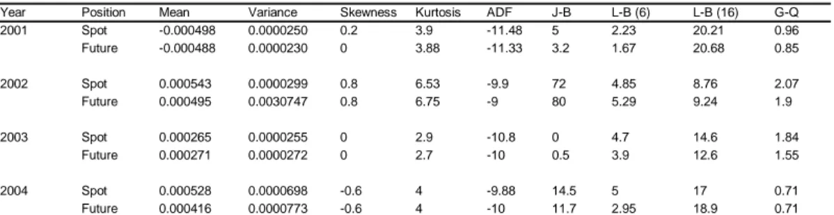
The statistics for the Copper spot and futures contract during the years 2001-2004 can be seen in table 1 below. The kurtosis presents some evidence of a leptokurtic distri-bution, with a non-normal distribution of the data in two of the four years. The skewness is close to zero at all contracts, which implies a symmetric distribution. These findings go in line with Byström (2000) and Baillie and Myers (1991) that commodity prices often are non-normally distributed. However, we will later show that the situation for the other commodities in this study is somewhat different. The Augmented Dickey-Fuller (ADF) test provides clear evidence that the time-series are stationary and the Goldmand-Quand (G-Q) shows that two of the years are ho-moscedastic, and two years are slightly heteroscedastic. This means that the variance for the spot and the futures contract are similar over time during the time period
ex-amined in this thesis. This is somewhat surprising and in contrast to several other studies (Byström, 2000; Baillie & Myers, 1991). However, the reason for the contra-diction is probably because we use time-series data of 6 months; where there is less likely to be large changes in variance over time, due to economic changes.
The Ljung-Box (L-B) statistics provides evidence that no autocorrelation is found in either the spot or the futures market, which is similar to the data in Baillie and Myers (1991). However, this is in contrast to Byström (2000) where autocorrelation was found in the futures market but not in the spot market.
The futures position in our study has a slightly higher variance than the spot position in three of the years.
Table 1 Copper statistics for June contracts 2001-2004
Year Position Mean Variance Skewness Kurtosis ADF J-B L-B (6) L-B (16) G-Q
2001 Spot -0.000498 0.0000250 0.2 3.9 -11.48 5 2.23 20.21 0.96 Future -0.000488 0.0000230 0 3.88 -11.33 3.2 1.67 20.68 0.85 2002 Spot 0.000543 0.0000299 0.8 6.53 -9.9 72 4.85 8.76 2.07 Future 0.000495 0.0030747 0.8 6.75 -9 80 5.29 9.24 1.9 2003 Spot 0.000265 0.0000255 0 2.9 -10.8 0 4.7 14.6 1.84 Future 0.000271 0.0000272 0 2.7 -10 0.5 3.9 12.6 1.55 2004 Spot 0.000528 0.0000698 -0.6 4 -9.88 14.5 5 17 0.71 Future 0.000416 0.0000773 -0.6 4 -10 11.7 2.95 18.9 0.71
The critical values for Augmented Dickey-Fuller (ADF), the test for non-stationary data, on the 0.01 level is -3.4. The critical values for 0.01 for Ljung-Box (L-B), the test for autocorrelation, are 31.99 for lag 16 and 16.8 for lag 6. The critical value for Jarque-Bera (J-B), the test for normality, is 9.21 on the 0.01 level. The Goldmand-Quand (G-Q), the test for homoskedasticity, critical values is 1.54 on the 0.05 level
4.1.2 Gold
The test statistic for Gold is very close to the data presented for Copper above. How-ever, this will be presented briefly below.
The statistics for the Gold spot and futures contracts during the years 2001-2004 can be seen in table 2 below. The kurtosis values presents evidence of a leptokurtic distri-bution for most contracts. The Jarque-Bera (J-B) test provides mixed results where most of the contracts are non-normally distributed. This is similar to Copper and goes in line with Byström (2000) and Baillie and Myers (1991).
The Augmented Dickey-Fuller (ADF) test provides clear evidence that the time-series are stationary and the Goldmand-Quand (G-Q) shows that all years are homoscedas-tic. This means that the variance for the spot and the futures contract are similar over time during the time period examined in this thesis. This is in line with the data for Copper but in contrast to several other studies as mentioned earlier.
The Ljung-Box (L-B) statistics provides evidence that no autocorrelation is found in either the spot or the futures market, which is similar to the data in Baillie and Myers (1991). However, this is in contrast to Byström (2000) where autocorrelation was found in the futures market but not in the spot market.
The futures position in our study has higher variance in two of the four years.
Table 2 Gold statistics for June contracts 2001-2004
Year Mean Variance Skewness Kurtosis ADF J-B L-B (6) L-B (16) G-Q
2001 Spot 0.0000154 0.0000197 1.8 16.5 -11 936.6 15.6 19.6 0.4 Future -0.000053 0.0000181 1 8.4 -10 159 10.7 19.4 0.5 2002 Spot 0.000506 0.0000128 0 3.67 -10.6 2.2 3.3 19 1.22 Future 0.000472 0.0000126 0.3 3.9 -10 5.9 5.5 19.7 1.21 2003 Spot 0.00204 0.0000223 -0.6 3.79 -9.8 10.75 5.1 16.4 1.53 Future 0.000162 0.0000239 -0.4 3.02 -11.7 2.76 6.2 24.6 1.61 2004 Spot -0.000329 0.0000179 -0.2 2.6 -9.4 1.6 6.7 21 0.76 Future -0.000358 0.0000252 -0.95 4.15 -11 23.4 4 17.7 1
The critical values for Augmented Dickey-Fuller (ADF), the test for non-stationary data, on the 0.01 level is -3.4. The critical values for 0.01 for Ljung-Box (L-B), the test for autocorrelation, are 31.99 for lag 16 and 16.8 for lag 6. The critical value for Jarque-Bera (J-B), the test for normality, is 9.21 on the 0.01 level. The Goldmand-Quand (G-Q), the test for homoskedasticity, critical values is 1.54 on the 0.05 level
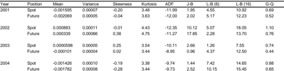
4.1.3 Cotton
The statistics for Cotton #2 spot and futures contract during the years 2001-2004 can be seen in table 3 below. The kurtosis, skewness and Jarque-Bera (J-B) values present evidence of a symmetric and normal distribution for all contracts except one. This is in contrast to several other studies and also somewhat different to Copper and Gold where at least two were non-normally distributed with leptokurtic distribution. However, the other test statistic presented below is similar to Gold and Copper. The Augmented Dickey-Fuller (ADF) test provides clear evidence that the time-series are stationary and the Goldmand-Quand (G-Q) shows that all years are homoscedas-tic, similar to the case for Gold and Copper. This means that the variance for the spot and the futures contract are similar over time during the time period examined in this thesis.
The Ljung-Box (L-B) statistics provides evidence that no autocorrelation is found in either the spot or the futures market, which is similar to the case of Copper and Gold as discussed above.
The futures contract has a lower variance than the spot position all years except one.
Table 3 Cotton #2 statistic for June contracts 2001-2004
Year Position Mean Variance Skewness Kurtosis ADF J-B L-B (6) L-B (16) G-Q 2001 Spot -0.001595 0.00007 -0.20 3.48 -11.99 1.95 4.55 10.92 0.69 Future -0.002069 0.00005 -0.04 3.63 -12.00 2.02 5.17 12.23 0.52 2002 Spot 0.000883 0.00011 -0.01 4.43 -12.35 10.12 5.07 18.05 1.10 Future 0.000339 0.00066 0.38 4.75 -11.27 17.85 2.28 13.70 0.76 2003 Spot 0.0000598 0.00005 0.25 3.54 -10.11 2.66 1.26 7.55 0.74 Future -0.000101 0.00004 0.02 3.44 -8.95 0.96 4.37 12.50 0.44 2004 Spot -0.001426 0.00010 -0.19 3.38 -9.74 1.44 7.42 14.65 0.88 Future -0.001782 0.00008 -0.28 3.44 -9.73 2.52 10.15 15.45 0.65 The critical values for Augmented Dickey-Fuller (ADF), the test for non-stationary data, on the 0.01 level is -3.4. The critical values for 0.01 for Ljung-Box (L-B), the test for autocorrelation, are 31.99 for lag 16 and 16.8 for lag 6. The critical value for Jarque-Bera (J-B), the test for normality, is 9.21 on the
0.01 level. The Goldmand-Quand (G-Q), the test for homoskedasticity, critical values is 1.54 on the 0.05 level
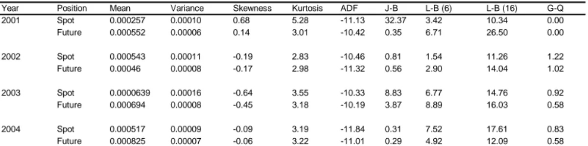
4.1.4 Oil
The statistics for Oil Light Crude spot and futures contract during the years 2001-2004 can be seen in table 4 below. The kurtosis and skewness values present evidence of a symmetric and normal distribution for most contracts. Similar as for Cotton, most of the contracts are normally distributed.
The Augmented Dickey-Fuller (ADF) test provides clear evidence that the time-series are stationary and the Goldmand-Quand (G-Q) shows that all years are homoscedas-tic, similar to the other commodities examined. This means that the variance for the spot and the futures contract are similar over time during the periods examined in this thesis.
The Ljung-Box (L-B) statistics provides evidence that no autocorrelation is found in either the spot or the futures market, which is similar to the case of the other com-modities.
The futures contract has a lower variance than the spot position during all years.
Table 4 Oil Light Crude statistic for June contracts 2001-2004
Year Position Mean Variance Skewness Kurtosis ADF J-B L-B (6) L-B (16) G-Q 2001 Spot 0.000257 0.00010 0.68 5.28 -11.13 32.37 3.42 10.34 0.00 Future 0.000552 0.00006 0.14 3.01 -10.42 0.35 6.71 26.50 0.00 2002 Spot 0.000543 0.00011 -0.19 2.83 -10.46 0.81 1.54 11.26 1.22 Future 0.00046 0.00008 -0.17 2.98 -11.32 0.56 2.90 14.04 1.02 2003 Spot 0.0000639 0.00016 -0.64 3.55 -10.33 8.83 6.77 14.76 0.92 Future 0.000694 0.00008 -0.45 3.18 -10.19 3.87 8.89 16.03 0.58 2004 Spot 0.000517 0.00009 -0.09 3.19 -11.84 0.31 7.52 17.61 0.83 Future 0.000825 0.00007 -0.06 3.22 -11.01 0.29 4.92 12.09 0.58 The critical values for Augmented Dickey-Fuller (ADF), the test for non-stationary data, on the 0.01 level is -3.4. The critical values for 0.01 for Ljung-Box (L-B), the test for autocorrelation, are 31.99 for lag 16 and 16.8 for lag 6. The critical value for Jarque-Bera (J-B), the test for normality, is 9.21 on the 0.01 level. The Goldmand-Quand (G-Q), the test for homoskedasticity, critical values is 1.54 on the 0.05 level.
4.1.4.1 Summary of the General Statistics
The variance for the spot and futures data set generated mixed result for the various commodities, where the Oil and Copper generated a higher variance for the futures for most years whereas Cotton and Gold had a mixed result between the years, where the futures where higher in some years but lower in some other. Common is that the variance is very close between the futures and spot, which is expected since the spot and futures contracts often follow each other closely.
Most of the spot and futures time-series above have normally distributed data, al-though with some leptokurtic characteristics. Oil and Cotton has a more symmetric and normal distributed data than Gold and Copper.
All time series for spot and futures where found to be stationary, where also most of the data sets are proven to be homoscedastic i.e. the variance is constant over time. This is in contrast to previous studies, where longer time periods than 6-months have been examined. Since we focused on a 6-month hedging decision, which is a relative short period, it is not surprising that the variance is constant over time. No autocor-relation was found in either short or long lags in the spot and the futures time series. Based on the above tests, we can conclude that since the time-series are stationary with a close to constant variance over time and close to normally distributed data for most time-series, we can continue by using an ordinary least squares regression and a minimum variance model to analyse the optimal hedge ratio and risk reduction for the different commodities. Thus, using more elaborate methods such as the GARCH framework will not be necessary and will therefore not be used in this thesis.
4.2 Optimal Hedge Ratio and Risk Reduction
In this section the optimal hedge ratio (OHR) and risk reduction for the five modities are presented. There are four different portfolios examined for each com-modity: the unhedged i.e. buying in the spot market, the Naive i.e. a fully hedged po-sition (100%), the ordinary least square (OLS) hedge ratio and the minimum variance (MV) hedge ratio.
In this part we focus on the OHR calculated by the OLS and MV in order to analyse what may be the OHR for each commodity. The variance will also be examined since this gives evidence which portfolio that may reduce the variance most effec-tively. The risk reduction parameter is important since it presents how much, in per-centage, that a portfolio may reduce the risk compared to the unhedged portfolio. In addition to this, we will have a general discussion how companies exposed to risk in these commodity may offset this risk.
4.2.1 Copper
The four different portfolios for Copper during the time period 2001-2004 can be seen in table 5 below.
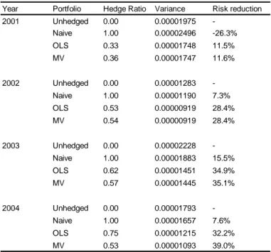
Table 5 Copper OHR and Risk Reduction
Year Portfolio Hedge Ratio Variance Risk reduction 2001 Unhedged 0.00 0.0000250 -Naive 1.00 0.0000017 93.2% OLS 0.94 0.0000018 92.7% MV 1.00 0.0000017 93.2% 2002 Unhedged 0.00 0.0000299 -Naive 1.00 0.0000018 93.8% OLS 0.99 0.0000018 93.9% MV 0.96 0.0000018 94.0% 2003 Unhedged 0.00 0.0000255 -Naive 1.00 0.0000018 92.9% OLS 1.02 0.0000019 92.5% MV 0.92 0.0000016 93.6% 2004 Unhedged 0.00 0.0000698 -Naive 1.00 0.0000114 83.6% OLS 0.98 0.0000111 84.1% MV 0.88 0.0000103 85.3%
The different years provides evidence of similar hedge ratios for the minimum vari-ance (MV) and the ordinary least squares (OLS). The span of the OHR is 88%-102% with an average of 96%. Since the OLS and MV are close to 100% for all years the best strategy is to consider a fully hedged position. Since the OHR is calculated as be-ing close to one, the Naive hedge performs equally well in reducbe-ing the variance for all years and companies does not have to consider leaving any portion of their expo-sure unhedged. The companies that are dependent on Copper either as a input or output should hence, based on the time-series examined in this thesis, remain fully hedged or at least around 90%.
The unhedged position generates higher variance for all years, which is naturally since the OHR is considered to be close to one. Hence, it is not recommended for companies to remain unhedged since exposure to Copper volatility may imply higher costs in their production, with lower margins as a result. Copper is the world third most used metal and is primarily used in industries such as construction and indus-trial machinery manufacturing (NYMEX, 2005). Hence, copper is vital for many corporations active in these industries, both as input in their production process and as an output for suppliers active in these industries.
The price levels of Copper spot and futures can be seen in Appendix 1, where a clear backwardation relationships is presents i.e. the spot is higher than the futures price. Hence, the mining industry may be reluctant to hedge futures since they would not prefer to lock in a price lower than the current spot price, whereas companies de-pendent on Copper in their production process would gain from lower futures prices compared to the current spot prices. Whatever the case may be, the metal processing industry profits and the share prices of the companies in this industry is a direct func-tion of the market prices of the commodities (FICCI, 2005).
4.2.2 Gold
The four different portfolios for Gold during the time period 2001-2004 can be seen in table 6 below.
Table 6 Gold OHR and Risk Reduction
Year Portfolio Hedge Ratio Variance Risk reduction 2001 Unhedged 0.00 0.00001975 -Naive 1.00 0.00002496 -26.3% OLS 0.33 0.00001748 11.5% MV 0.36 0.00001747 11.6% 2002 Unhedged 0.00 0.00001283 -Naive 1.00 0.00001190 7.3% OLS 0.53 0.00000919 28.4% MV 0.54 0.00000919 28.4% 2003 Unhedged 0.00 0.00002228 -Naive 1.00 0.00001883 15.5% OLS 0.62 0.00001451 34.9% MV 0.57 0.00001445 35.1% 2004 Unhedged 0.00 0.00001793 -Naive 1.00 0.00001657 7.6% OLS 0.75 0.00001215 32.2% MV 0.53 0.00001093 39.0%
The MV and OLS hedge ratios generate similar values for all years, with risk reduc-tion significantly higher than the Naive hedge in all cases. The OHR is in the span of 33%-75%, with an average of 52%. The Naive hedge reduces the variance better for Gold than for Copper when comparing the different portfolio alternatives. This is true with the exception of 2001 where it is better to remain unhedged than consider-ing a Naive hedge. In this year, the Naive hedge generates a negative risk reduction due to the large variance, which has also been seen in Satyanarayan et al. (1994) where the Naive hedge in some cases caused a negative risk reduction.
Baillie and Myers (1991) generated an OHR of 50% for the OLS hedge and a hedge ratio of 30%-60% using the GARCH framework, with only small variations over time. This goes in line with the OHR of Gold in our models.
The unhedged position performed almost equally well in reducing the variance as the Naive hedge. The OLS and the MV hedge reduced the variance slightly more than the other two portfolios. In strong contrast to Copper, corporations, governments and investors do not gain as much from hedging Gold contracts as the case for the other commodities studied, even though some of the risk exposure can be reduced. Gold futures contracts are used in many different commercial and industrial areas; concentration of gold is found in association with copper and lead in a vide range of products. Gold is an excellent conductor of electricity making it widely used in elec-tronics and other high-tech applications. As in the case for Copper, a wide range of
companies uses the futures contract as a hedging instrument, from mining companies to fabricators of finished products (NYMEX, 2005).
In the case of the crude oil markets the market is often in backwardation, which is of-ten referred to as a reason why oil majors do not hedge. In the Gold market it is the opposite, where the market is often in contango. Hence, many gold producers have regularly hedged their production forward, partly to pick up the contango (Cameron, 2002). Our data of Gold spot and futures on the price level also provides evidence of a somewhat contango effect i.e. the futures price is higher than the spot (see appendix 2). However, this is only marginal and Gold is the commodity in this study where spot and futures prices follow each other most closely. Hence, a small variation be-tween the spot and futures prices implies a smaller hedge ratio compared to the other commodities.
Mining companies within the Gold and Copper industry have a commodity risk ex-posure foremost on the output side, where they supply Gold or Copper to their cus-tomers. This can successfully be offset by futures hedging with significant risk reduc-tion as a result. In addireduc-tion, mining companies may also be exposed to commodity inputs required for the mining process. This can be oil fuel, gas and electricity that is necessary to supply power to the mines (Cameron, 2002). Hence, it is important to hedge these exposures as well.
4.2.3 Cotton
The four different portfolios for Cotton #2 during the time period 2001-2004 can be seen in table 7 below.
Table 7 Cotton OHR and Risk Reduction
Year Portfolio Hedge Ratio Variance Risk reduction 2001 Unhedged 0.00 0.00007160 -Naive 1.00 0.00001152 83.9% OLS 0.78 0.00001624 77.3% MV 1.10 0.00001103 84.6% 2002 Unhedged 0.00 0.00011018 -Naive 1.00 0.00001348 87.8% OLS 0.75 0.00002522 77.1% MV 1.22 0.00001015 90.8% 2003 Unhedged 0.00 0.00005100 -Naive 1.00 0.00000709 86.1% OLS 0.80 0.00000985 80.7% MV 1.09 0.00000680 86.7% 2004 Unhedged 0.00 0.00009623 -Naive 1.00 0.00000655 93.2% OLS 0.88 0.00000928 90.4% MV 1.08 0.00000606 93.7%
The hedge ratios for MV and OLS for Cotton have higher ratios than Copper and Gold, where all Cotton ratios are closer to 1. Also, the MV and OLS ratios provide evidence of different hedge ratios in several of the cases, where some has a value of
higher than one. Surprisingly, the Naive hedge performs better in reducing the vari-ance than the OLS for all years. However, the MV model reduced the varivari-ance slightly more than the Naive. The unhedged position has a higher variance in all years than the other portfolios.
Hence, for companies with an exposure to volatility in Cotton, the OHR is 75%-122% with an average of 96%. It is imperative to not remain unhedged since this gen-erates a significant higher variance than the other alternatives.
Our results are somewhat different than to the OHR of 38% that Baillie and Myers (1991) calculated for Cotton between January 1985 and July 1986. The reason for this may be that the time period used in our study is different both from the number of observations and the date when the study took place. The risk reduction and OHR for different types of Cotton by Satyanarayan et al. (1994) provides similar result as in our study, where the authors concluded that a risk reduction of over 50% was pre-sent, and in many cases up to 90%. Similar to the OHR for the MV model in our case, several of the OHR by Satyanarayan et al. (1994) also have a value higher than 1.
Similar to Satyanarayan et al. (1994) who argues that cotton dependent export coun-tries (the top five in the world is China, USA, India, Pakistan and Brazil (Cotton Outlook, 2005) can lower their risk exposure by engaging in the futures market, our analysis views the same picture where the variance can significantly be reduced with hedging in the futures market. This should be considered for companies in emerging countries that can engage in the futures market to hedge their future cash flows. This is especially critical for Cotton since the harvesting season occurs only during a cer-tain time period, where hence a large portion of that year’s cash flow is generated. It can clearly be seen in Appendix 3 that a contango effect is present between the spot and future price levels, i.e. the futures price is higher than the spot price. This implies that Cotton producers may benefit from the contango effect in the short-run.
To hedge risk exposure in Cotton is also important for companies active in industries that are dependent on cotton either as input or output in the production process, for example in the textile industry. This is especially crucial in the textile industry since it is difficult to pass on price increases to consumers. However, these companies may slightly be negatively affected by the contango effect in the short-run (Cotton Out-look, 2005).
4.2.4 Oil
The four different portfolios for Oil Light Crude during the time period 2001-2004 can be seen in table 8 below.
Table 8 Oil Light Crude OHR and Risk reduction
Year Portfolio Hedge Ratio Variance Risk reduction 2001 Unhedged 0.00 0.0005531
-Naive 1.00 0.0002459 55.5% OLS 0.58 0.0002956 46.6% MV 0.98 0.0002456 55.6% 2002 Unhedged 0.00 0.0005979