Urban biodiversity; a global perspective.

(1)

U

RBAN BIODIVERSITY

;

A GLOBAL

PERSPECTIVE

Isaac Awuku Acheampong

July 2013

TRITA-LWR Degree Project 13:37

ISSN 1651-064X

(2)

Isaac Awuku Acheampong TRITA LWR Degree Project 13.37

ii © Isaac Awuku Acheampong

Degree Project for Master’s program in Environmental Engineering and Sustainable Infrastructure

Department of Land and Water Resources Engineering Royal Institute of Technology (KTH)

SE-100 44 STOCKHOLM, Sweden

Reference should be written as: Acheampong, I A (2013) “Urban biodiversity; a global perspective” TRITA LWR Degree Project.13:37. 28p.

(3)

iii DEDICATION

This project is dedicated to Mr. Kwabena Kesse, popularly known as Kessben. Without him, I couldn’t have travelled to Sweden to begin this MSc program.

(4)

(5)

v

S

UMMARY IN

S

WEDISH

Majoriteten av världens städer är belägna i eller nära områden med hög biodiversitet. Den ökande andel av befolkningen som bor i städer globalt sett har resulterat i en snabb urban expansion, vilken kan utgöra ett hot mot urban biodiversitet och kan därigenom få konsekvenser för den ekologiska balansen och människors välbefinnande. Urban biologisk mångfald är därför en viktig faktor att ta hänsyn till i utvecklingen av våra städer. När den urbana mångfalden påverkas, påverkas ekosystemtjänster också. Ekosystemtjänster är förmåner och tjänster som människor erhåller från ekosystem, vilka består av alla levande organismer och relaterade icke-levande miljöer. Det blir därför viktigt att få fram tillräckligt med information om utvecklingen i ekosystemen och miljön genom tillförlitliga och konsekventa indikatorer.

Det främsta syftet med denna studie är att jämföra ett antal städer över världen med hjälp av globala datamängder för att kunna mäta urban biologisk mångfald, vilket är en hållbarhetsfråga som är har hög politisk relevans. I studien ingick 102 städer över hela världen och fokus för analysen var områden belägna inom 15 km och 30 km från städernas centra.

Den rumsliga analysen gjordes i GIS-programmet ArcGIS 10. Data från MODIS och GLOBCOV som användes för analysen omklassades för att huvudsakligen fokusera på urban markanvändning, naturlig vegetation och jordbruksmark. Baserat på denna omklassning analyserades varje stad med avseende på andel markanvändning för varje markanvändningsklass i 15 km och 30 km buffertzoner. En regressionsanalys utfördes också med växt- och fågelarter som responsvariabler, som analyserades i relation till andel urban markanvändning och annan markanvändning. Resultaten visade bland annat att städer med stor befolkning och högre andel urban markanvändning hade lägre andel naturlig vegetation, och vice versa. Regressionsanalysen visade att utbredningen av urban markanvändning influerade antal fågelarter och antal inhemska fågelarter (p<0.05). På liknande sätt påverkades också antal växtarter och antal inhemska växtarter av urban markanvändning (p<0.05). Dessutom visade resultaten, att båden inom 15 km och 30 km hade andel och fragmentering av naturlig vegetation inverkan på antal växtarter. Detta var dock inte fallet med fågelarter.

Sammanfattningsvis kan den allmänna trenden med hög andel urban markanvändning och låg andel naturlig vegetation i och kring städer ses som oroande. Det tyder på att den kontinuerliga ökningen av stadsbefolkningen sannolikt kommer att förvärra situationen ytterligare, vilket resulterar i höga krav på städernas ekologiska fotavtryck och ekosystemtjänster som helhet. Eftersom biologisk mångfald i städerna har betydelse för ekosystemtjänster och människors hälsa, behöver dessa indikatorer kontinuerligt övervakas och utvecklas, samtidigt som de behöver relateras till möjligheter att bevara naturliga ekosystem och dess funktioner i stadsnära miljö.

"Endast genom att förstå miljön och hur den fungerar, kan vi ta de nödvändiga besluten för att skydda den. Endast genom att värdera alla våra värdefulla naturresurser och mänskliga resurser kan vi hoppas att bygga en hållbar framtid. " – Kofi Annan, fore detta generalsekreterare för FN.

(6)

(7)

vii

S

UMMARY IN

E

NGLISH

A majority of the world’s cities are situated in or near areas of high biodiversity. Rise in global urban population resulting in rapid urban expansions (larger cities) is a threat to urban biodiversity, which has implications for the ecological health and general wellbeing of humans. Urban biodiversity is thus an important factor in the development of our cities. When urban biodiversity is affected, ecosystem services are also affected. Ecosystem services are benefits or services humans derive from the ecosystem, which is made up of all living organisms and the non-living environments. It therefore becomes essential to provide adequate information about trends in the ecosystem and environmental conditions in general by way of reliable and consistent indicators.

The main objective of the study is to compare a number of cities across the globe using global data sets for a measure of urban biodiversity, a sustainability concern of high policy relevance. The study involved 102 cities across the globe, and the focus of the data analysis was within 15 km and 30 km buffers from the approximate centres of the cities. The spatial analysis was conducted in a Geographic Information System (GIS). The MODIS and GLOBCOV data used for the analysis was reclassified to mainly focus on urban land use with respect to artificial developments, natural habitat and agriculture. Based on this reclassification, each city was analysed for the percentage of land use for each component within the 15 km and 30 km buffers. Regression analysis was also performed with plants and birds species as response variables to the percentage of urban land use and the other reclassified components.

The results show among other things that cities with high population and higher percentage of land use dedicated to artificial infrastructure recorded lower percentage size of natural habitat, and vice versa. The regression analysis with total and native birds as response variables to percentage urban size as predictor shows a significant level of influence as the p-values were less than 0.05. Similarly, total and native plant species are also influenced significantly by both percentage urban and natural habitat. In these regression analyses within 15 km and 30 km, p-values were less than 0.05. Furthermore, the results show that within both 15 km and 30 km, the percentage size of natural habitat and number of patches has a significant effect on the number of plant species. This was however not the case with regards to bird species. In conclusion, the general trend of high urban extent resulting in low percentage of natural habitat within the cities can be seen as worrying. It suggests that the continual increasing of urban population is likely to further aggravate the situation, resulting in unbearable demands on the cities ecological footprints and ecosystem services as a whole. Thus the more our cities grow; the further humanity may be separated from nature. Since urban biodiversity has implications for human and ecological health, its indicators must be constantly measured and monitored, while adhering to best practices that conserve nature.

“Only by understanding the environment and how it works, can we make the necessary decisions to protect it. Only by valuing all our precious natural and human resources can we hope to build a sustainable future.” – Kofi Annan, Former UN Secretary General.

(8)

(9)

ix

A

CKNOWLEDGEMENTS

I express my sincerest gratitude to Ulla Mörtberg (assistant professor), my advisor, for her support, encouraging advice and constructive suggestions. Her inputs, comments and suggestions immensely enriched the content of this study, and I am thankful.

I am grateful to my parents, family and friends for their support and encouragement. Their presence around me gives me a sense of purpose and fulfillment. Of particular mention are Rita Ansah Quagrain, Jemima Kusi Asare and Nana Kwasi Anaisie, for standing with me in difficult moments. I appreciate the efforts of Isaac Owusu-Agyeman, my friend and brother. I will forever cherish our union and friendship. To Felix Osei Bonsu, and Peter Amoah Tawiah, thank you very much for your outstanding support. A special word of thanks to Jan Haas of the Geoinformatics department, KTH for his assistance, and also to all who in diverse ways assisted me in this study.

(10)

(11)

xi

A

CRONYMS AND ABBREVIATIONS

CIESIN Centre for International Earth Science Information Network ESRI Environmental Systems Research Institute

FR Full Resolution

GIS Geographic Information System

GPWv3 Gridded Population of the World, Version 3 LCCS Land Cover Classification System

MEA Millennium Ecosystem Assessment MERIS Medium Resolution Imaging Spectrometer MODIS Moderate Resolution Imaging Spectrometer SEDAC Socioeconomic Data and Application Centre UN United Nations

(12)

(13)

xiii

T

ABLE OF

C

ONTENTS

Dedication ... iii

Summary in Swedish ...v

Summary in English ... vii

Acknowledgements ... ix

Acronyms and abbreviations... xi

Table of Contents ... xiii

Abstract ... 1

1. Introduction ... 1

1.1. Problem Statement ... 2

1.2. Objectives of the study ... 2

2. Background... 2

2.1. Indicators... 2

2.2. Urban Biodiversity ... 3

2.3. Ecosystem services ... 3

3. Materials and Methods ... 4

3.1. Materials ... 4

3.1.1. Study area ... 4

3.1.2. Data ... 4

3.1.3. Description of datasets ... 5

3.1.4. Population data ... 5

3.1.5. Programs and Software ... 7

3.2. Methods ... 7 3.2.1. Cities ... 7 3.2.2. Buffers ... 7 3.2.3. Data Processing ... 7 3.2.4. Data Reclassification ... 7 3.2.5. Data Analysis ... 9 3.2.6. City Population ... 11 3.2.7. Fragmentation ... 12 3.2.8. Predictor-Response Model ... 13

4. Results and Discussion ... 14

4.1. Land cover composition in the cities ... 14

4.1.1. GLOBCOVER ... 14

4.1.2. MODIS... 15

4.2. GLOBCOVER versus MODIS ... 15

4.3. Patch metrics ... 21 4.4. Regression analysis ... 22 4.5. General Discussion ... 24 5. Conclusion ... 25 References ... 26 Other References ... 27

(14)

(15)

1

A

BSTRACT

A majority of the world’s cities are situated in or near areas of high biodiversity. Rise in global urban population resulting in rapid urban expansions (larger cities) is a threat to urban biodiversity, which has implications for the ecological health and general well being of humans. The study exploits consistent global land use data to compare 102 cities across the globe on a measure of urban biodiversity, within 15 km and 30 km from the approximate centres of the cities. Cities with high population and higher percentage of land use dedicated to artificial infrastructure recorded lower percentage size reserved for natural habitat, and vice versa. Further testing in regression analysis with birds and plants species as response variables shows a relation with urban extent and size of natural habitat which seeks to promote sustaining ecosystems services. Since urban biodiversity has implications for human ecological health, its indicators must be constantly measured and monitored, while adhering to best practices that conserve nature.

Keywords: Urban biodiversity; Indicators; Ecosystem services; Fragmentation; Regression analysis.

1. I

NTRODUCTION

“I view great cities as pestilential to the morals, the health, and the liberties of man.” - Thomas Jefferson

Can man in anyway separate himself from his environment? To a larger extent, the environment as well as quality of life for humanity and the natural world is determined by our association with cities (Hoornweg et al., 2006). As we fashion out cities that are ecologically sustainable, there is a need to develop passable environmental indicators capable of providing resource for urban planning (Stanley, 2008), management decision-making and policy formulation (Donnelly et al., 2007). This is necessitated by current trends which anchor that socioeconomic development vis-à-vis the concept of ecological cities should be based on sustainable development (Rudisser et al., 2012; Stanley, 2008). Tanguay et al., (2010) as well as several other publications reckon that sustainable development encompasses the environmental, social and economic, and as far back as the United Nations (1992) conference that enacted the Agenda 21, the need for sustainable development indicators to aid in decision making is accentuated.

A critical aspect of ecology of cities is biodiversity conservation in the long term (Balmford et al., 2005), where indicators are essential to assess anthropogenic influence on biodiversity (Rudisser et al., 2012). Ultimately, in the long term analysis, human wellbeing is central to conserving biodiversity and its services. This is the underpinning factor for the convention on biological diversity’s 2010 target, when in 2002 at the World Summit on Sustainable Development in Johannesburg, the governments represented committed themselves to “….achieving by 2010 a significant reduction of the current rate of biodiversity loss at the global, regional and national level…” (UNEP, 2002). Of similar importance in the features of ecology in cities is a measure of energy use and energy efficiency, which is a key in activating fundamental social and economic activities in the cities (Keirstead and Schulz, 2010). However, in recent times ‘acceptability’ of energy policies (Schiffer, 2008) is pre-requisite for a robust sustainable energy future (Shell, 2008).

This study set the tone for a comparative study between cities on biodiversity efficiency; a sustainability issue of high policy relevance in recent times.

(16)

2

1.1. Problem Statement

Many user organizations of environmental indicators including the World Bank bemoan the disaggregated nature of available city indicators, which are mostly unreliable and non-comparable across cities and over time (Hoornweg et al., 2006). It is becoming increasingly difficult to substantiate information provided by these indicators due to the absence of robustness in the selection process of the indicators (Dale and Beyeler, 2001). This calls for a systematic approach in the process of selection and development of environmental indicators (Niemeijer and de Groot, 2008). Though this systems approach has been applied in the past (Bossel, 2001), Niemeijer (2002) opines there is need for improvement in the indicator selection process in order to achieve effective and consistent corroboration of indicators (Bockstaller and Girardin, 2003). Comparability of these environmental indicators across cities globally over time, as well as consistency in the use of global datasets remains a major challenge.

In related studies, while Keirstead and Schulz (2010) recommended a dynamic framework for the analysis of cities with respect to energy use and energy efficiency paying particular attention to “understanding diversity”, Rudisser et al (2012) suggests developing highly intelligible environmental indicators to support the ‘planning and evaluation of policies’ that have direct consequence on biodiversity.

1.2. Objectives of the study

The main objective of the study is to compare a number of cities across the globe using global data sets for a measure of urban biodiversity, a sustainability concern of high policy relevance.

The study has the following specific objectives;

• To define the percentage component of relevant land use class within 15 km and 30 km from the centre of the cities, as a measure of fragmentation

• To assess the effect of urban activities on biodiversity within the urban extents

•

To test statistically through regression and residual analysis the relation between anthropogenic factors such as urban extents as predictors and plant/bird species richness as response within the cities.

2. B

ACKGROUND

2.1. Indicators

Different definitions abound for environmental indicators; however, the prime focus is their ability to provide adequate information about trends in the ecosystem and environmental conditions in general. “Indicators” can be explicated as a degree of a relevant environmental phenomena used to appraise environmental conditions (Heink and Kowarik, 2010). The European Environmental Agency (2005) also defines indicators as a measure usually quantitative that is used to basically exemplify complex phenomenon. An environmental indicator according to the USEPA (2010) is defined as “a numerical value that helps provide insight into the state of the environment”. These implies that environmental indicators are required to be measurable and valid scientifically, so as to provide some form of authentic verification of trends in quality with respect to the ecosystem and environment in general (Donnelly et al., 2007). It is also important that the environmental indicators fashioned out are able

(17)

3

to act as a tool to assess the interactions between various sectors and players in the city and their ecosystems environment.

The framers of the UN Agenda 21 at the Rio conference were spot-on in emphasising the crucial role of environmental indicators in achieving sustainability in our cities, which led to the documentations of some guidelines towards achieving this goal (UN, 1992). However, even right from inception of the concept of indicators, the challenge of modalities, consistency, reliability and comparability across cities over time were intimated. The use of global datasets GlobCov & MODIS can be a way forward to enhance the comparability, stability and reliability of environmental indicators. Their capacity to aid decision makers in evaluating existing systems of sustainability in the cities is also expected to improve

.

2.2. Urban Biodiversity

Urban biodiversity is an important factor in the development of our cities. It is even more of global extent as sustainability and preservation of species and reserves are largely dependent on the urban environments. That is, commercial and residential areas / activities greatly impact green urban infrastructure (Hostetler et al., 2011). In as much as individual actions are crucial to the operation and maintenance of preserved natural areas, Hostetler and Noiseux (2010) suggested that many who lived in such preserved regions lacked this understanding. Considering the rate of springing up of big cities where artificial built up systems are gradually taking over natural native systems through urbanization (Pickett et al., 1997), a lot of species are in danger of been extinct (Olden et al., 2005), as well as other negative effect on other habitat fragmentation parameters, and this pose a worrying threat to biodiversity in so many ways (Turner et al., 2004). Much therefore need to be done through the use of indicators and effective monitoring to achieve plausible management goals as far as this aspect of sustainability is concerned (Mulder et al., 1999, Thompson 2006). Even though the use of indicators to direct reserves and forest management has attracted many criticisms in the past (e.g., Prendergast et al., 1993, Carignan and Villard, 2002, etc.), yet many other studies including McLaren et al., (1998), Lindenmayer, (1999), Carignan and Villard, (2002), among others agree that there is a need for some form of indicators. Thompson, (2006) particularly submits that it is difficult to surmise sustainability without the use of indicators and monitoring. The key concern here is the use of systems thinking and robustness in the selection and definition of environmental indicators for such purposes, which are a major focus and an integral part of this study.

2.3. Ecosystem services

All living organisms (plants, animals and humans) and the non-living environment interact to form a complex known as the ecosystem (MEA, 2005). It is often said that the well being of humans is largely dependent on the kind of services benefited from ecosystems, widely known as ecosystem services. Ecosystem services can therefore be simply defined as the benefits or services humans gain from ecosystems. This is proportioned into four different forms, namely provisioning, regulating, cultural and supporting services. This concept of ecosystems services was formalized in 2005 by the United Nations in its Millennium Ecosystem Assessment (MEA, 2005). As population growth with its associated expansion of urban areas increases human demands on natural resources, the global ecological footprint is overstretched, and

(18)

4

chiefly affected is urban biodiversity. Ecosystems services are thus so fundamental to human life, such that its depletion and degradation has staid repercussion. However, if the very essence of preserved and well managed ecosystems services is to be appreciated, then planned expansion of cities and urban areas is to be oriented towards achieving it, and primly to be considered is urban biodiversity. In the design of the conceptual framework for the millennium assessment, the pivotal hub was placed on human well being and biodiversity, identifying that, decisions by humans on ecosystems have their well being as central (MEA, 2005).

3. M

ATERIALS AND

M

ETHODS

The various methods employed in carrying out the study are comprehensively dealt with in this chapter. It also presents the materials used in the study such as data, sources of data, programs and software as well as the study area.

3.1. Materials

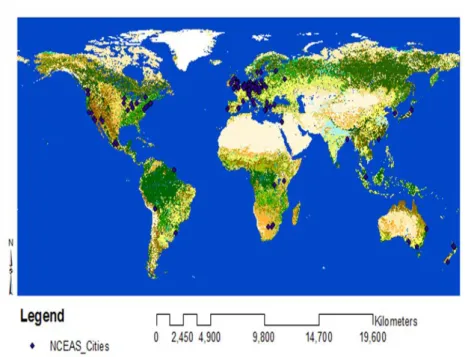
3.1.1. Study area

The study covers 102 cities across the globe, with majority of the cities within Europe. There were no particular criteria for selecting the cities covered in the study, except based on the availability of biodiversity data. However, all the six continents were covered. As many cities as possible were covered to ensure a very broad base for the comparison the study seeks to do. The map layout and list of the cities are presented in figure 1 and appendix A respectively.

3.1.2. Data

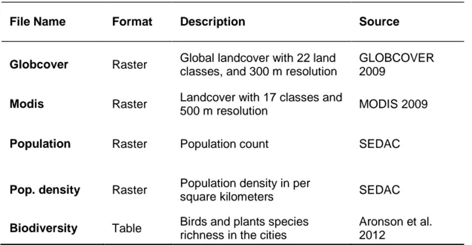
The following data were used in the study. They include global raster datasets for input into a Geographic Information System (GIS) (Table 1), as well as statistical population and population density figures of the cities. Data on number of birds and plants for each city was collected from Aronson et al. 2012.

(19)

5 3.1.3. Description of datasets

Globcover

The Globcover 2009 land cover map is a 300 m resolution land cover map of global extent produced from the Medium Resolution Imaging Spectrometer (MERIS) Full Resolution (FR) time series and classified according to United Nations (UN) Land Cover Classification System (LCCS), (Bontemps et al., 2010). The map has 22 land cover types which are well documented, highly reliable and comparable globally (Bontemps et al., 2010).

Modis

The MODIS data is a map of urban extent covering the globe of 500 m pixel size. It was produced by the MODIS land group and associate partners to present a current map of urban, settled and built up areas of the land surface of the earth. The map was produced using Moderate Resolution Imaging Spectrometer (MODIS) data at a spatial resolution of 1km, and has a total of 17 land cover classes (Scheneider et al., 2003). In developing the map, urban extents were defined as areas where more than 50% the land space is covered by human made surfaces such as roads, infrastructure etc, and all non-vegetative elements. That is, adjoining patches of built-up land greater than one square kilometre was considered urban (Scheneider et al., 2009). According to Scheneider et al., (2009), accuracy appraisal pegs the MODIS 500 m map as the most pragmatic presentation of global urban land use, which is also validated, consistent, and comparable globally and can serve as the basis for advanced global urban land use depiction.

3.1.4. Population data

The population and population density grid data, available as “Gridded Population of the World, Version 3”, was prepared by the Centre for International Earth Science Information Network (CIESIN), Columbia University and published through the Socioeconomic Data and Application Centre (SEDAC). The population count grid estimates human population for the year 2010 by 2.5 arc-minute grid cells through the number of persons per grid. Subsequently, the population density grids are obtained by dividing the population count by land area representing persons per square kilometre.

Table 1: Data used.

File Name Format Description Source

Globcover Raster Global landcover with 22 land _{classes, and 300 m resolution} GLOBCOVER ₂₀₀₉

Modis Raster Landcover with 17 classes and _{500 m resolution} MODIS 2009

Population Raster Population count SEDAC

Pop. density Raster Population density in per _{square kilometers} SEDAC

Biodiversity Table Birds and plants species

richness in the cities

Aronson et al. 2012

(20)

6

(21)

7 3.1.5. Programs and Software

The main software used for the study was the GIS program ArcGIS version 10 from ESRI (ESRI 2008). GIS is particular useful for integration of data from different sources and formats, as well as for spatial analysis. All geographic data processing, spatial analysis, spatial statistics, patches and landscape metrics computation were carried out in ArcGIS, while Microsoft Excel was used for some of the statistics computations and graphs. All regression analysis and plots of the data were carried out using the software MINITAB.

3.2. Methods

3.2.1. Cities

All the cities under study were captured in ArcGIS as points. The points represented the approximate centres of the cities, around which major urban functionalities and activities revolve.

3.2.2. Buffers

In ArcGIS, buffer zones of 15 km and 30 km were created around the city centre points. For most of the time, the question remains unanswered what the exact boundaries of cities are; so for the purpose of this study, all data capture and subsequent analysis was restricted to 15 km and 30 km radii from the approximate centres of the cities. 3.2.3. Data Processing

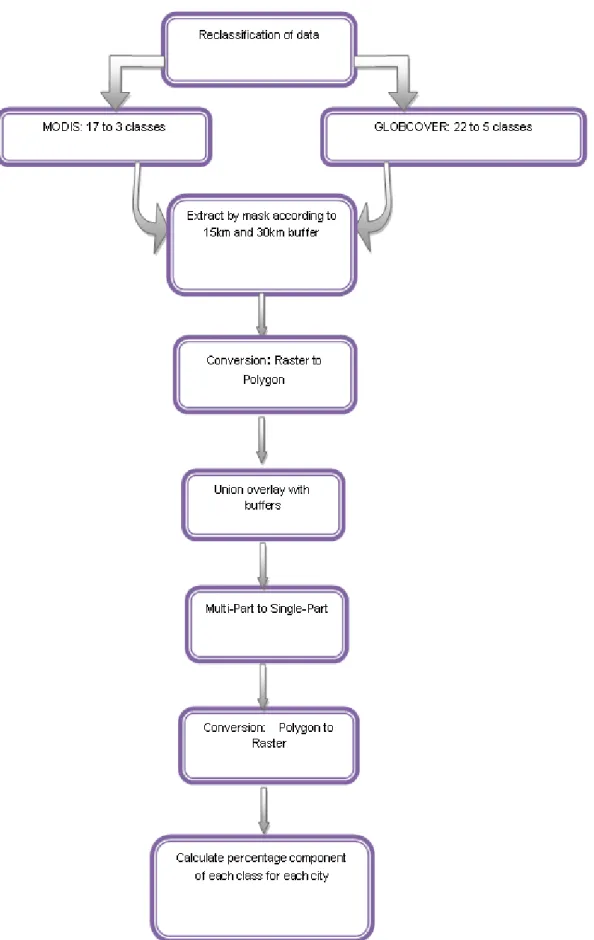
The summary of the data processing is presented in figure 2. 3.2.4. Data Reclassification

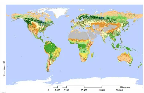
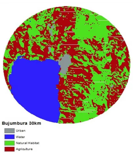
The original GLOBCOVER data (Fig. 3) with 22 classes of different land cover uses (Table 2) was reclassify into 5 interesting classes of land cover uses, namely urban, water, natural habitat, agriculture and others (Table 3). Particular attention was paid to mosaics of land uses which were largely considered as natural habitat or relatively undisturbed nature reserves / vegetation. This reclassification was necessary due to the primary focus of the study on biodiversity efficiency in the cities being considered. The map of the reclassified GLOBCOVER data is presented in figure 4.

Figure 3: GLOBCOVER map (300 m pixel size) with 22 land use classes (Source: GLOBCOVER 2009).

(22)

8

Table 2: Original classes and codes for GLOBCOVER data.

CODE Description

11 Post-flooding or irrigated croplands (or aquatic) 14 Rainfed croplands

20 Mosaic cropland (50-70%) / vegetation (grassland/shrubland/forest) (20-50%)

30 Mosaic vegetation (grassland/shrubland/forest) (50-70%) / cropland (20-50%)

40 Closed to open (>15%) broadleaved evergreen or semi-deciduous forest _(>5m) 50 Closed (>40%) broadleaved deciduous forest (>5m)

60 Open (15-40%) broadleaved deciduous forest/woodland (>5m) 70 Closed (>40%) needleleaved evergreen forest (>5m)

90 Open (15-40%) needleleaved deciduous or evergreen forest (>5m) 100 Closed to open (>15%) mixed broadleaved and needleleaved forest (>5m) 110 Mosaic forest or shrubland (50-70%) / grassland (20-50%)

120 Mosaic grassland (50-70%) / forest or shrubland (20-50%) 130 Closed to open (>15%) (broadleaved or needleleaved, evergreen or

deciduous) shrubland (<5m)

140 Closed to open (>15%) herbaceous vegetation (grassland, savannas or lichens/mosses)

150 Sparse (<15%) vegetation

160 Closed to open (>15%) broadleaved forest regularly flooded (semi-_{permanently or temporarily) - Fresh or brackish water} 170 Closed (>40%) broadleaved forest or shrubland permanently flooded -

Saline or brackish water

180 Closed to open (>15%) grassland or woody vegetation on regularly flooded or waterlogged soil - Fresh, brackish or saline water

190 Artificial surfaces and associated areas (Urban areas >50%) 200 Bare areas

210 Water bodies

220 Permanent snow and ice 230 No data (burnt areas, clouds,…)

(23)

9

Subsequently, the MODIS data of urban extent covering the Globe (Fig. 5) with 17 classes of land cover uses (Table 4) was reclassified into 3 classes (Table 5), namely water, urban and non-urban. In the reclassification of the MODIS data, the focus was on what is urban, and what is non-urban since urban extent is the prime focus of this MODIS dataset. Therefore, apart from what is defined and considered as urban, and water, all others was grouped under the class non-urban. The resulting map is presented in figure 6.

3.2.5. Data Analysis

The data was analysed using ArcGIS. Using the reclassified GLOBCOVER and MODIS data as input and the city buffers of 15 km and 30 km as input feature mask data with the Spatial Analyst Tool in ArcGIS, the features of the reclassified datasets within the buffers were extracted. The extracted raster data were vectorized and subsequently united with resulting polygon shapefiles for both GLOBCOVER and MODIS, and for the city buffers of 15 km and 30 km.

The output data from this operation was a table with the attributes of the city buffers, as well as the GLOBCOVER data and MODIS data. In this way each city was linked to the specific features of GLOBCOVER and MODIS within 15 km and 30 km from the approximate centres of the cities. Using the data management tool ‘multipart to singlepart’, and ‘select by attributes’ from the resulting attribute table, all features relating to each city under both GLOBCOVER and MODIS within both 15 km and 30 km buffers were selected, and the selected features exported to separate shapefiles.

Table 3: Reclassified classes of GLOBCOVER data.

Value Description GLOBCOVER code

1 Urban areas, artificial surfaces and

associated areas 190 2 Water bodies 210, 170, 180 3 Natural habitat 40, 50, 60, 70, 90, 100, 110, 120, 130, 140, 150, 160 4 Agriculture 11, 14, 20, 30 5 Others 200, 220, 230

(24)

10

Table 4: Original classes and codes for MODIS map.

CODE Description

0 Water

1 Evergreen needleleaf forest

2 Evergreen broadleaf forest

3 Deciduous needleleaf forest

4 Deciduous broadleaf forest

5 Mixed forest 6 Closed Shrubland 7 Open shrubland 8 Woody savanna 9 Savanna 10 Grassland 11 Permanent wetland 12 Cropland 13 Urban

14 Cropland natural vegetation mosaic

15 Snow and ice

(25)

11

This was performed separately for the 15 km buffer both for GLOBCOVER and MODIS data, and for the 30 km buffer both for GLOBCOVER and MODIS as well.

Thus for each of the 102 cities buffers of both 15 km and 30 km, relating features were exported into a taseparate shapefile for that city for each of the two datasets being analysed. Each of the cities polygon shapefiles were then converted to raster for both GLOBCOVER with 5 classes and MODIS with 3 classes for both 15 km and 30 km buffers (e.g. Fig. 7). The raster datasets was re-projected using Lambert projections for the continents under which each city falls. The percentages of each component of GLOBCOVER and MODIS within the 15 km and 30 km buffers of each city were calculated.

3.2.6. City Population

Even though various statistical institutions of the various countries and city boards have published data of estimated population, area and population density of the cities, they were not considered wholly definite and well defined for the purpose of this study. This is due to the Figure 5: MODIS map (500 m pixel size) with 17 land use classes (Source: MODIS land group, 2009).

(26)

12

unanswered issue of actual boundaries of population counts of cities within countries, besides, all data analysis were restricted to 15 km and 30 km radius from the approximate centres of the cities, hence the need to define both population and population density of the cities according to the same radius. In this respect, total population and population density of the cities were estimated from the population and population density grid data respectively. This was done by estimating the total count of population from cells within the buffers of the cities. Zonal statistics was performed in ArcGIS to obtain the population and population density of each city within both 15 km and 30 km buffer zones.

3.2.7. Fragmentation

For a study like this which focuses on biodiversity efficiency, measures of fragmentation are essential for a better understanding. For the purpose of this study, two fragmentation parameters were used; percentage of habitat/land cover as well as the landscape metric Table 5: Reclassified classes of MODIS map.

Value Description MODIS code

0 Water 0

1 Urban 13

2 Non-urban 1 - 12, 14 - 16

Figure 7: Land use classes representation within 30 km of Bujumbura.

(27)

13

parameter ‘number of patches’ within the buffers for each city, computed in ArcGIS. A patch represents an area or polygon within a map covered by a particular land cover class (Eiden et al., 2000). From the polygon shapefile of features extracted by the buffers from the GLOBCOVER data of 5 classes, the interesting feature classes namely urban, water, natural habitat and agriculture were exported to a separate shapefile for each of these classes and for both buffers. The polygon shapefiles of each feature class was subsequently converted to raster. By performing zonal statistics on the raster maps for each feature class (urban, water, natural habitat, agriculture), the number of patches of each feature class for each city within both 15 km and 30 km buffer zones were recorded.

3.2.8. Predictor-Response Model

With the biodiversity data on plants and birds, the purpose was to model their response to the various components of the landcover in the cities as predictors. Thus a regression analysis was carried out using the number of birds and plants as response variables, and the interested land cover classes, namely size of urban, natural habitat, number of patches of natural habitat and human population as predictors. This was done for both the 15 km and the 30 km buffers. All regression analysis was done using MINITAB.

For bird response analysis, total number of bird species as a response variable was regressed against percentage urban as the only predictor,

(28)

14

and subsequently the residuals from this analysis was used as response and regressed against percentage natural habitat as predictor, number of patches of natural habitat as predictor and combined percentage natural habitat and number of patches of natural habitat as additional predictor. This was repeated with the number of native bird species, and the whole process as above repeated for plants as response variable, both total number of plant species and number of native plant species. The results of all the analysis and statistical components were recorded to a table.

4. R

ESULTS AND

D

ISCUSSION

This section provides the results for the various spatial analyses and statistics carried out for the study.

4.1. Land cover composition in the cities

4.1.1. GLOBCOVER

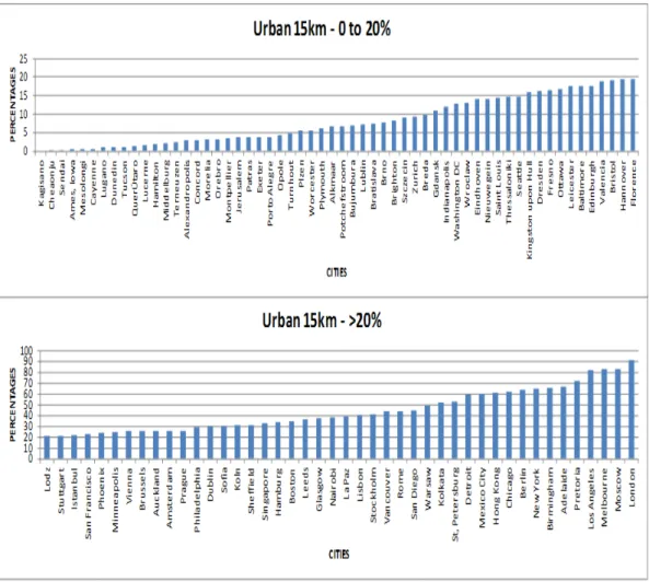
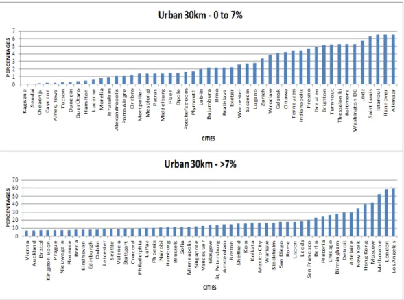
The representation of all cities in terms of percentages of urban, water, natural habitat, agriculture and other are recorded in. The cities are covered on the average with 23.7% and 10.4% urban, 11.2% and 12.7% water, 38.9% and 45.5% natural habitat, 25.9% and 31% agriculture within the 15 km and 30 km buffers respectively. The graphical representation of all landcover classes for all cities is presented in figures 8-15. Apart from water and agriculture, all cities were fairly covered with urban extents and natural habitat. Most developed cities in Europe and Northern America has a higher urban percentage compared to the developing cities in Africa and Asia. Consequently, the pattern shows a reverse situation for size of natural habitat. For a majority of the cities with higher urban extent, the size of natural habitat is low, and the reverse also holds (Fig. 16). This trend invariably has dire consequence for size of natural habitat extents in the cities as urbanization increases and cities continue to grow, and confirms the long held perception and Figure 9: Percentage of water within 15km.

(29)

15

fears that urban expansion is at the expense of conservation of natural vegetation. How cities are planned and fashioned out is critical to preserving the size of natural habitat extent, and for that matter related biodiversity, in the cities.

4.1.2. MODIS

The results of the MODIS data analysis of percentage of water, urban and non-urban were recorded to a table. The prime component of the MODIS data analysis is a measure of urban extents for the cities, which recorded an average of 36.1% and 17.1% within 15 km and 30 km respectively. Percentages of non-urban on the average for all cities were 55.5% and 71.0% within 15 km and 30 km respectively.

4.2. GLOBCOVER versus MODIS

A conspicuous trend from the results of the analysis of both GLOBCOVER and MODIS data is a decrease in the urban extents of the cities moving from 15 km buffer from the approximate centres of the cities into the 30 km buffer (Fig. 17).

Conversely, natural habitat/non-urban extents increase from the 15 km buffer to the 30 km buffer for majority of the cities. This suggests a probable trend where the design, planning, and development of the cities are oriented towards shifting biodiversity from the nucleus of the cities. Even though both GLOBCOVER and MODIS map are of global extents, the results from both data analysis show some differences in urban extents within the buffers for the cities (Fig. 18). This could be attributed to the interpretation and definition of what is defined and considered as urban. Mapping of urban areas is always extremely difficult Figure 10: Percentage of Natural Habitat within 15km.

(30)

16

due to the assorted nature of land use forms in urban settings (Schneider et al., 2009). It is worth noting that the main focus of the MODIS map is

Figure 12: Percentage of urban within 30km. Figure 11: Percentage of Agriculture within 15km.

(31)

17

Figure 13: Percentage of water within 30km.

(32)

18

Figure 15: Percentage of Agriculture within 30km.

(33)

19

Table 6: Regression parameters predictors of birds and plant species within 15km and 30km buffer from the centre of the cities

BIRD ANALYSIS 15KM BUFFER

Predictor Response Coefficient F P R-sq

% Urban Total Birds 0.46 9.19 0.004 16.10% % Natural Habitat Residuals -0.37 0.91 0.35 1.90% Number of Patches of Natural Habitat Residuals -0.05 0.19 0.668 0.40% Combined % Natural Habitat and Number of

patches of Natural habitat Residuals -0.46//-0.09 0.74 0.484 3% % Urban Native Birds 1.36 9.24 0.004 16.10% % Natural Habitat Residuals -0.33 0.74 0.39 1.50% Number of Patches of Natural Habitat Residuals -0.05 0.17 0.68 0.40% Combined % Natural Habitat and Number of

patches of Natural habitat Residuals -0.42//-0.08 0.62 0.544 2.60%

BIRD ANALYSIS 30KM BUFFER

% Urban Total Birds 0.99 5.31 0.026 10% % Natural Habitat Residuals -0.38 0.86 0.36 1.80% Number of Patches of Natural Habitat Residuals -0.018 0.29 0.59 0.60% Combined % Natural Habitat and Number of

patches of Natural habitat Residuals -0.64//0.05 1.1 0.34 4.50% % Urban Native Birds 2.201 5.12 0.028 9.60% % Natural Habitat Residuals -0.33 0.69 0.411 1.40% Number of Patches of Natural Habitat Residuals -0.017 0.25 0.616 0.50% Combined % Natural Habitat and Number of

patches of Natural habitat Residuals -0.57//-0.05 0.91 0.411 3.70%

PLANT ANALYSIS 15KM BUFFER

% Urban Total Plants 7.71 6.55 0.013 10.50% % Natural Habitat Residuals 5.11 3.18 0.08 5.40% Number of Patches of Natural Habitat Residuals -1.71 3.21 0.079 5.40% Combined % Natural Habitat and Number of

patches of Natural habitat Residuals 3.47/1.17 2.18 0.122 7.40% % Urban Native plants 6.03 7.49 0.008 11.80% % Natural Habitat Residuals 4.27 4.23 0.044 7.00% Number of Patches of Natural Habitat Residuals -1.36 3.81 0.056 6.50% Combined % Natural Habitat and Number of

patches of Natural habitat Residuals 3.03/-0.882 2.76 0.072 9.10%

PLANT ANALYSIS 30KM BUFFER

% Urban Total Plants 10.9 4.4 0.04 7.30% % Natural Habitat Residuals 6.5 4.51 0.038 7.50% Number of Patches of Natural Habitat Residuals -0.66 7.03 0.01 11.20% Combined % Natural Habitat and Number of

patches of Natural habitat Residuals 3.21/-0.521 3.92 0.026 12.50% % Urban Native plants 9.26 5.98 0.018 9.60% % Natural Habitat Residuals 5.41 6.07 0.017 9.80% Number of Patches of Natural Habitat Residuals -0.535 8.99 0.004 13.80% Combined % Natural Habitat and Number of

(34)

20

Figure 18: Difference in percentage urban land cover from MODIS and GLOBCOVER data for all cities.

Figure 17: Comparing %urban land cover within 15 km and 30 km buffer for MODIS and GLOBCOVER.

(35)

21

urban extents. Despite the differences, the key factor is the consistency in the data, and their global extents which makes the comparable study more reliable and relevant.

4.3. Patch metrics

The number of patches for each land use class was recorded. However, the number of patches of natural habitat is further used as a predictor in the predictor-response model for birds and plant species.

Figure 19: Bird regression plots within 15 km buffer

A. Total birds versus % urban .

B. Native birds versus % urban .

C. Residual total birds versus % natural habitat and number of patches.

(36)

22

4.4. Regression analysis

The results of the regression analysis show a positive correlation between size of urban extent and total birds as well as number of native birds in both 15 km (Fig. 19) and 30 km (Fig. 20) buffers, however a stronger correlation within 15 km from the centre of the cities (Table 6). This suggests that the reported bird species were by instruction being recorded in from larger areas in larger cities. Subsequently, the results further show that there is no correlation between the number of bird species and the size of natural habitat or number of patches of natural habitat or both within 15 km and 30 km as well (Fig. 19, 20). This means

Figure 20: Bird species regression plots 30 km buffer

A. Total birds versus % urban .

B. Native birds versus % urban .

C. Residual total birds versus % natural habitat and number of patches.

(37)

23

that the urban areas, carefully structured and managed, can accommodate higher number of bird species and individuals as well. Similarly, the regression of total plant species and number of native plants against size of urban extent of the cities within both 15 km and 30 km buffers shows a positive correlation (Fig. 21, 22). Contrary to the situation with birds species, the plant species regression analysis further show a positive relation with size of natural habitat but however shows a negative correlation with number of patches of natural habitat. The significance level of these correlations is further determined by the p-values obtained in the analysis. Here, p-values less than 0.05 (Table 6) are considered significant. Within 15 km and 30 km, analysis with both total and native birds as response to percentage of urban size produce p-values less than 0.05 (Table 6). This shows that there is a significant level of influence of bird species presence by the percentage size of urban within the cities. However, total and native plant species are significantly influenced by both percentage of urban and natural habitat, as the p-values for these analysis within 15 km and 30 km are less than 0.05 (Table 6). The trend in these results tends to promote a cohabitation individuals and larger size of natural habitat preserved, which Figure 21: Plant species regression plots within 15 km buffer

A. Total plants versus % urban.

B. Native plants versus % urban.

C. Residual total plants versus % natural habitat and number of patches.

(38)

24

consequently can host larger species of plants. Eventually, the concept of ecosystems services is upheld in this case as well. The statistical parameters of all the regression analyses are presented in table 6.

4.5. General Discussion

By 2010, 50.6% of the world’s human population lived in urban areas and cities (UN, 2008). It is further predicted that that by 2050, more than 70% would be living in cities (UN, 2008, Chan et at., 2010). The analysis of the data in this study reveals that increase in urban size and population leads to a reduction in the size of natural habitat in the cities, and it is increasingly evident that at this rate the ecological footprint of many cities is outstretched and largely unsustainable (Kareiva et al., 2007). To some extent, the results and analysis of the study suggest that improved resource for planning and management decision making is crirical to biodiversity conservation in the long term, as prescribed in previous studies (E.g. Donnelly et al., 2007 and Stanley, 2008). Even though in addition to human activities, natural systems also contributes to fragmentation of habitat (Pickett and Thompson, 1978), which in-fact is actually loss of habitat (Andren, 1994), it is widely believed that a consistent measure of urban biodiversity to be achieved even as cities expand is essential in saving the natural habitat. Interestingly, the regression analysis of birds and plant species provides a soothing. The expanding urban areas with relatively low size of natural habitat have capacity to host larger number of plant and bird species. This could be explained by the fact that new habitats created by humans have the

Figure 22: Plant species regression plot within 30 km buffer

A. Total plants versus % urban.

B. Native plants versus % urban.

C. Residual total plants versus % natural habitat and number of patches.

(39)

25

potential of increasing the presence of species in the habitat (Andren, 1994), even at this, plant species richness require a larger size of natural habitat within urban areas. This perhaps suggests that promoting the integration of urban expansion and biodiversity conservation is a useful step towards building sustainable cities.

As an indicator to guide decision makers, city authorities and planners, the question is asked of whether it is prudent to set a fixed target of a percentage of urban land use for biodiversity preservation. In his review of the effects of habitat fragmentation on birds and mammals in landscapes with different proportions of suitable habitat, Andren (1994) suggested that preserving about 30% of suitable habitat of a landscape is of much relevance. However it is still not absolute in determining the pattern of growth/expansion since considerations for ecosystem services would require integration of nature reserves with human settlements rather than maintaining the two separately.

5. C

ONCLUSION

The use of global data sets for the analysis in the study yielded essential results, consistent enough to form the basis of a reliable comparison of the cities across the globe on a measure of urban biodiversity. In the overall, all cities are fairly represented in terms of urban extent, natural habitat, agriculture, water and others. The general trend of high urban extent resulting in low percentage of natural habitat within the cities is worrying. It suggests that the continual increasing of urban population is likely to further aggravate the situation, resulting in unbearable demands on the cities ecological footprints and ecosystem services as a whole. Thus the more our cities grow; the further humanity is separated from nature.

The plants and birds species samples used in the regression test analysis suggest a relation with urban extents and size of natural habitat, especially for plant species, where size of natural habitat within the cities is critical. These inclinations explicate the concept of ecosystem services which promotes mutual coexistence between humans and their ecosystem. Without this, generations to come may not have the prospect to appreciate nature and also gain from it.

In the light of these, studies based on a systems approach and scientific principles for testing indicator species and other relevant variables for assessing extent of urban biodiversity loss must be austerely pursued, both city wide and globally, with inherent monitoring programs. This awareness must of a necessity influence the orientation of city authorities towards building sustainable cities. A change that must not be seen as an obstacle to rapid development, but a challenge accepted by all in preserving the diminishing urban biodiversity.

(40)

26

R

EFERENCES

Andren, H., 1994. Effects of habitat fragmentation on birds and mammals in landscapes with different proportions of suitable habitat: A review Oikos, 71 (3), 355 – 366.

Balmford, A., Bennun, L., ten Brink, B., Cooper, D., Cote, I.M., Crane, P., Dobson, A., Dudley, N., Dutton, I., 2005. The Convention on Biological Diversity’s 2010 Target. Science 307, 212– 213.

Bockstaller, C., Girardin, P., 2003. How to Validate Environmental Indicators. Agric. Syst. 76, 639 – 653

Bossel, H., 2001. Assessing Viability and Sustainability: A Systems-based Approach for Deriving Comprehensive Indicator Sets. Conserv. Ecol. 5, 12.

Carignan, V. and Villard, M.A., 2002. Selecting indicator species to monitor ecological integrity: a review. Environmental Monitoring and Assessment 78, 45 – 61.

Dale, V.H., Beyeler, S.C., 2001. Challenges in the Development and Use of Ecological Indicators. Ecological Indicators 1, 3 – 10.

Donnelly, A., Jones, M., O’Mahony, T., Byrne, G., 2007. Selecting Environmental Indicator for Use in Strategic Environmental Assessment. Environmental Impact Assessment Review 27, 161 – 175.

Eiden, G., Kayadjanian, M., Vidal, C., 2000. Capturing landscape structures; Tools. In: From land cover to landscape diversity in the European Union.

Heink, U., Kowarik, I., 2010. What are Indicators? On the Definition of Indicators in Ecology and Environmental Planning. Ecological Indicators 10, 584 – 593.

Hoornweg, D., Nuñez, F., Freire, M., Palugyai, N., 2006. The World Bank; Third World Urban Forum, Vancouver.

Hostetler, M.E., Noiseux, K., 2010. Are green residential developments attracting environmentally savvy homeowners? Landscape Urban Plan. 94, 234–243.

Hostetler, M., Allen, W., Meurk, C., 2011. Conserving Urban Biodiversity? Creating Green Infrastructure is only First Step. Landscape and Urban Planning 100, 369 – 371

Kareiva, P., Watts, S., McDonald, R., Boucher, T., 2007. Domesticated nature: Shaping landscapes and ecosystems for human welfare. Science 316, 1866 – 1869.

Keirstead, J. and Schulz, N. B., 2010. London and Beyond: Taking a Closer Look at Urban Energy Policy. Energy Policy 38, 4870 – 4879. Lindenmayer, D.B., 1999. Future directions for biodiversity conservation

in managed forests: indicator species, impact studies and monitoring programs. Forest Ecology and Management 115, 277 – 287.

MEA (Millennium Ecosystem Assessment), 2005. Ecosystems and Human Well-Being: A Framework for Assessment. Island Press, Washington, 155pp

McLaren, M.A., Thompson, I.D., Baker, J.A., 1998. Selection of vertebrate wildlife indicators for monitoring sustainable forest management in Ontario. The Forestry Chronicle 74, 241 – 248.

Mulder, B.S., Noon, B.R., Spies, T.A., Raphael, M.G., Palmer, C.J., Olsen, A.R., Reeves, G.H., Welsh, H.H., 1999. The strategy and

(41)

27

design of the effectiveness monitoring program for the Northwest Forest Plan. USDA Forest Service, Pacific Northwest Forest Station, General Technical Report PNW – GTR – 437. 138p.

Niemeijer, D., 2002. Developing Indicators for Environmental Policy: Data-driven Approaches examined by Example. Environ. Sci. Policy 5, 91 – 103.

Niemeijer, D., de Groot R.S., 2008. A Conceptual Framework for Selecting Environmental Indicator Sets. Ecological Indicators 8, 14 – 25.

Olden, J.D., Douglas, M.R., Douglas, M.E., 2005. The human dimensions of biotic homogenization. Conservation Biology 19, 2036 – 2038.

Pickett, S.T.A., Thompson, J.H., 1978. Patch dynamics and the design of nature reserves. Biological Conservation 13, 27 – 37.

Pickett, S., Burch, W., Dalton, S., Foresman, T., Morgan, J., Rowntree, R., 1997. A Conceptual framework for the study of human ecosystems in urban areas. Urban Ecosystems 1, 185 – 199.

Prendergast, J.R., Quinn, R.M., Lawton, J.H., Eversham, B., Gibbons, D.H., 1993. Are species, the coincidence of diversity hotspots and conservation strategies? Nature 365, 335 – 337.

Rudisser, J., Tasser, E., Tappeiner, U., 2012. Distance to Nature – A New Biodiversity Relevant Environmental Indicator Set at the Landscape Level. Ecological Indicators 15, 208 – 216.

Schiffer, H.W., 2008. WEC Energy Policy Scenarios to 2050. Energy Policy 36 (7), 2464 – 2470.

Schneider, A., Friedl M.A., Potere, D., 2009. A new map of global urban extent from MODIS data. Environmental Research Letters 4, article 044003.

Schneider, A., Friedl M.A., Potere, D., 2010. Monitoring urban areas globally using MODIS 500m data: New methods and datasets based on urban eco-regions. Remote Sensing of Environment 114, 1733 – 1746.

Shell, 2008. Shell Energy Scenarios to 2050. Technical Report, Shell International.

Stanley, C. T. Yip, 2008. Planning for Eco-Cities in China, 44th ISOCARP Congress.

Tanguay, A., Lefebvre, J.F., Lanoie, P., 2010. Measuring the Sustainability of Cities: An Analysis of the Use of Local Indicators. Ecological Indicators 10, 407 – 418.

Thompson, I.D., 2006. Monitoring Of Biodiversity Indicators in Boreal Forests: A Need For Improved Focus. Environmental Monitoring and Assessment 121, 263 – 273.

Turner, W.R., Nakamura, T., Dinetti, M., 2004. Global Urbanization and separation of human from nature. BioScience 54, 585 – 590.

United Nations, 1992. Agenda 21: The United Nations Programme of Action from Rio. United Nations, New York.

Other References

Bontemps, S., Defourny P., Van B. E., 2010. Globcover 2009, Products

Description and Validation Report. https://globcover.s3.amazonaws.com/LandCover2009/GLOBCOV

(42)

28

Chan, L., Yap, W., 2010. The Singapore index on cities’ biodiversity. Second Curitiba meeting on cities’ biodiversity, Curitiba. http://www.cbd.int/authorities/doc/mayors-02/Wendy-Yap-en.pdf [Accessed 08/03/2012] http://www.trivia-library.com/b/u-s-president-thomas-jefferson-quotes-from-jefferson.htm [Accessed 12/01/2012] http://www.capital- biodiversity.eu/uploads/media/Indicators_for_urban_biodiversity_-_GUIDELINES_-_European_Capitals_of_Biodiversity.pdf [Accessed 08/03/2012] http://sage.wisc.edu/people/schneider/research/data_readme.html [Accessed:11/05/2012] http://www.millenniumassessment.org/documents/document.48.aspx.p df [Accessed:27/05/2012] http://www.esa.org/education_diversity/pdfDocs/ecosystemservices.p df [Accessed:27/05/2012]

United Nations, 2008. Population Division of the Department of Economic and Social Affairs of the United Nations Secretariat, World Urbanization Prospects: The 2007 Revision. http://esa.un.org/unup [Accessed 27/05/2012]

USEPA, 2010. http://www.epa.gov/igateway/whatIndicator.html [Accessed 15/01/2012]

(43)

I

A

PPENDIX

1:

L

IST OF CITIES

Table 1A: List of cities and their geographical locations.

CITY COUNTRY CONTINENT

Adelaide Australia Oceania Alexandropolis Greece Europe Alkmaar Netherlands Europe Ames, Iowa USA N. America Amsterdam Netherlands Europe Auckland New Zealand Oceania Baltimore USA N. America Berlin Germany Europe Birmingham UK Europe Boston USA N. America Bratislava Slovakia Europe Breda Netherlands Europe Brighton UK Europe

Bristol UK Europe

Brno Czech Republic Europe Brussels Belgium Europe Bujumbura Burundi Africa Cayenne French Guyana Europe Cheaonju South Korea Asia Chicago USA N. America Concord USA N. America Detroit USA N. America Dresden Germany Europe Dublin Ireland Europe Dunedin New Zealand Oceania Edinburgh UK Europe Eindhoven Netherlands Europe

Exeter UK Europe

Florence Italy Europe Fresno USA N. America Gdansk Poland Europe

Glasgow UK Europe

Hamburg Germany Europe Hamilton New Zealand Oceania Hannover Germany Europe Hong Kong China Asia Indianapolis USA N. America Istanbul Turkey Asia Jerusalem Israel Asia Kagisano South Africa Africa Kingston upon Hull UK Europe Kolkata India Asia Koln Germany Europe La Paz Bolivia S. America

Leeds UK Europe

Leicester UK Europe Lisbon Portugal Europe Lodz Poland Europe

London UK Europe

Los Angeles USA N. America Lublin Poland Europe Lucerne Switzerland Europe Lugano Switzerland Europe Melbourne Australia Oceania Mesolongi Greece Europe Mexico City Mexico N. America Middelburg Netherlands Europe Minneapolis USA N. America Montpellier France Europe Morelia Mexico N. America Moscow Russia Asia Nairobi Kenya Africa New York USA N. America Nieuwegein Netherlands Europe Opole Poland Europe

(44)

II

Orebro Sweden Europe Ottawa Canada N. America Patras Greece Europe Philadelphia USA N. America Phoenix USA N. America Plymouth UK Europe Plzen Czech Republic Europe Porto Alegre Brazil S. America Potchefstroom South Africa Africa Prague Czech Republic Europe Pretoria South Africa Africa QuerÚtaro Mexico N. America

Rome Italy Europe

Saint Louis USA N. America San Diego USA N. America San Francisco USA N. America Seattle USA N. America

Sendai Japan Asia

Sheffield UK Europe Singapore Singapore Asia Sofia Bulgaria Europe St, Petersburg Russia Asia Stockholm Sweden Europe Stuttgart Germany Europe Szczecin Poland Europe Terneuzen Netherlands Europe Thessaloniki Greece Europe Tucson USA N. America Turnhout Belgium Europe Valencia Spain Europe Vancouver Canada N. America Vienna Austria Europe Warsaw Poland Europe Washington DC USA N. America Worcester USA N. America Wroclaw Poland Europe Zurich Switzerland Europe