3D SYNTHETIC APERTURE FOR CONTROLLED-SOURCE
ELECTROMAGNETICS
by Allison Knaak
A thesis submitted to the Faculty and the Board of Trustees of the Colorado School of Mines in partial fulfillment of the requirements for the degree of Doctor of Philosophy (Geophysics). Golden, Colorado Date Signed: Allison Knaak Signed: Dr. Roel Snieder Thesis Advisor Golden, Colorado Date Signed: Dr. Terry Young Professor and Head Department of Geophysics
ABSTRACT
Locating hydrocarbon reservoirs has become more challenging with smaller, deeper or shallower targets in complicated environments. Controlled-source electromagnetics (CSEM), is a geophysical electromagnetic method used to detect and derisk hydrocarbon reservoirs in marine settings, but it is limited by the size of the target, low-spatial resolution, and depth of the reservoir. To reduce the impact of complicated settings and improve the detecting capabilities of CSEM, I apply synthetic aperture to CSEM responses, which virtually in-creases the length and width of the CSEM source by combining the responses from multiple individual sources. Applying a weight to each source steers or focuses the synthetic aperture source array in the inline and crossline directions. To evaluate the benefits of a 2D source distribution, I test steered synthetic aperture on 3D diffusive fields and view the changes with a new visualization technique. Then I apply 2D steered synthetic aperture to 3D noisy synthetic CSEM fields, which increases the detectability of the reservoir significantly. With more general weighting, I develop an optimization method to find the optimal weights for synthetic aperture arrays that adapts to the information in the CSEM data. The application of optimally weighted synthetic aperture to noisy, simulated electromagnetic fields reduces the presence of noise, increases detectability, and better defines the lateral extent of the tar-get. I then modify the optimization method to include a term that minimizes the variance of random, independent noise. With the application of the modified optimization method, the weighted synthetic aperture responses amplifies the anomaly from the reservoir, lowers the noise floor, and reduces noise streaks in noisy CSEM responses from sources offset kilometers from the receivers. Even with changes to the location of the reservoir and perturbations to the physical properties, synthetic aperture is still able to highlight targets correctly, which allows use of the method in locations where the subsurface models are built from only es-timates. In addition to the technical work in this thesis, I explore the interface between
science, government, and society by examining the controversy over hydraulic fracturing and by suggesting a process to aid the debate and possibly other future controversies.
TABLE OF CONTENTS
ABSTRACT . . . iii
LIST OF FIGURES AND TABLES . . . ix
ACKNOWLEDGMENTS . . . xvi
DEDICATION . . . xix
CHAPTER 1 GENERAL INTRODUCTION . . . 1
1.1 Thesis overview . . . 4
CHAPTER 2 SYNTHETIC APERTURE WITH DIFFUSIVE FIELDS . . . 9
2.1 Abstract . . . 9
2.2 Introduction . . . 9
2.3 3D Synthetic Aperture and Beamforming . . . 11
2.3.1 Numerical Examples . . . 13
2.4 3D Visualization . . . 17
2.4.1 Numerical Examples . . . 19
2.5 Discussion and Conclusions . . . 27
2.6 Acknowledgments . . . 27
CHAPTER 3 3D SYNTHETIC APERTURE FOR CSEM . . . 28
3.1 Abstract . . . 28
3.2 Introduction . . . 28
3.3 Mathematical basis . . . 30
3.5 Visualizing steered fields in 3D . . . 35
3.6 Conclusion . . . 38
3.7 Acknowledgments . . . 39
CHAPTER 4 OPTIMIZED 3D SYNTHETIC APERTURE FOR CSEM . . . 40
4.1 Abstract . . . 40
4.2 Introduction . . . 41
4.3 Weighted synthetic aperture . . . 42
4.4 Optimizing the weights for synthetic aperture . . . 43
4.5 Synthetic examples . . . 47
4.5.1 Increasing detectability . . . 49
4.5.2 Increasing lateral detectability . . . 53
4.6 Conclusion . . . 57
4.7 Acknowledgments . . . 57
CHAPTER 5 ERROR PROPAGATION WITH SYNTHETIC APERTURE . . . 58
5.1 Introduction . . . 58
5.2 Error propagation theory with synthetic aperture . . . 59
5.3 Reducing error propagation with optimization . . . 61
5.4 Synthetic example . . . 65
5.5 Conclusion . . . 76
5.6 Acknowledgments . . . 77
CHAPTER 6 THE SENSITIVITY OF SYNTHETIC APERTURE FOR CSEM . . . . 78
6.1 Introduction . . . 78
6.2.1 Perturbing the model . . . 80
6.2.2 Uncertainty in the location of the target . . . 89
6.3 Conclusion . . . 100
6.4 Acknowledgments . . . 101
CHAPTER 7 FRACTURED ROCK, PUBLIC RUPTURES: THE HYDRAULIC FRACTURING DEBATE . . . 102
7.1 Introduction . . . 102
7.2 Participatory models . . . 106
7.3 Background . . . 109
7.3.1 Entrance of hydraulic fracturing and regulations . . . 109
7.3.2 Key new technology . . . 111
7.3.3 Current practices . . . 112
7.3.4 Shale gas and major plays . . . 113
7.3.5 Current regulations . . . 116
7.4 The fracking debate . . . 118
7.4.1 Hydraulic fracturing documentaries . . . 122
7.5 Fracking as a post-normal technology . . . 126
7.5.1 System uncertainties . . . 126
7.5.2 Decision stakes . . . 130
7.6 Importance of Deliberation . . . 133
7.6.1 Challenges to a democratic approach . . . 134
7.6.2 Extended peer communities/extended participation model . . . 138
CHAPTER 8 GENERAL CONCLUSIONS . . . 143 REFERENCES CITED . . . 147
LIST OF FIGURES AND TABLES
Figure 1.1 A diagram showing the main components of synthetic aperture radar.
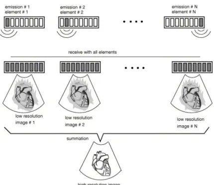
Taken from Avery & Berlin. . . 3 Figure 1.2 A diagram depicting synthetic aperture implemented in ultrasound
imaging. Taken from Jensen et al.. . . 4 Figure 2.1 The design of a traditional CSEM survey. The individual source, s1, is
defined to be located at the origin. The steering angle, ˆn, is a function of θ, the dip and ϕ which is either 0◦ or 90◦ to steer in the inline or
crossline directions, respectively. . . 14 Figure 2.2 The point-source 3D scalar diffusive field log-transformed with the
source at (0,0,0). . . 14 Figure 2.3 The unsteered 3D scalar diffusive field log-transformed. . . 15 Figure 2.4 The 3D scalar diffusive field log-transformed and steered at a 45◦ angle
in the inline direction. The arrow shows the shift in the x-direction of the energy from the origin; without steering the maximum energy
would be located at the center of the source lines (x= 0km). . . 16 Figure 2.5 The 3D scalar diffusive field log-transformed and steered at a 45◦ angle
in the crossline direction. The arrow shows the shift in the energy from the centerline of the survey (y= 0km). The shift is less than in . . . 16 Figure 2.6 The 3D scalar diffusive field log-transformed and steered at a 45◦ angle
in the inline and crossline directions. The arrows demonstrate the shift in the energy in the x- and y- directions. . . 17 Figure 2.7 The unwrapped phase of a scalar diffusive field from a point-source
located at (0,0,0). The colorbar displays radians. . . 19 Figure 2.8 The normalized gradient of a scalar diffusive field from a point-source
location at (0,0,0). . . 20 Figure 2.9 The phase-binned gradient of a scalar diffusive field from a point-source
located at (0,0,0). The change in direction occurs from the
Figure 2.10 The unwrapped phase of a scalar diffusive field with five lines of
synthetic aperture sources. The colorbar displays radians. . . 21 Figure 2.11 The normalized gradient of a scalar diffusive field with five synthetic
aperture sources. . . 21 Figure 2.12 The phase-binned gradient of a scalar diffusive field with five unsteered
synthetic aperture sources. The movement of the energy is symmetric
about both the x and y directions. . . 22 Figure 2.13 The phase-binned gradient of a scalar diffusive field with five synthetic
aperture sources steered in the inline direction at a 45◦. The energy is moving asymmetrically in the x-direction unlike the symmetric
movement of the unsteered field. . . 23 Figure 2.14 The phase-binned gradient of a scalar diffusive field with five synthetic
aperture sources steered in the crossline direction at 45◦. The energy is moving asymmetrically in the negative y-direction in contrast to the
symmetric movement of the unsteered field. . . 24 Figure 2.15 The phase-binned gradient of a scalar diffusive field steered in the inline
and crossline directions at 45◦. The combined inline and crossline steering produces a field whose energy moves out asymmetrically in
both the x- and y-directions. . . 25 Figure 2.16 The y-z view of the unsteered diffusive field, panel a), and the
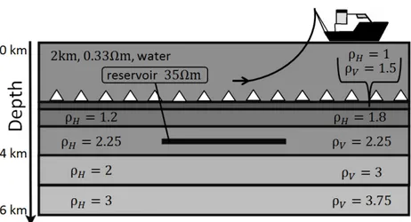
combined inline and crossline steered diffusive field, panel b), at a phase of 3π. The oval highlights the change in the direction of the field caused by steering. . . 26 Figure 3.1 The model used to create the synthetic CSEM data. The values of ρH
and ρV are the resistivity of the layer in the horizontal and vertical
direction respectively given in Ohm-meters. . . 33 Figure 3.2 The geometry of the CSEM survey for the synthetic data. The seven
towlines are shown as black lines. The reservoir is the black rectangle.
The 3D box outlines the coverage of the sampling points. . . 33 Figure 3.3 The ratio of the absolute value of the inline electric component for a
single source (panel a), a 2D synthetic aperture source (panel b), and a steered 2D synthetic aperture source (panel c). All three images depict the response at receivers located on the ocean floor. The footprint of the reservoir is outlined in black and the source is outlined in red. The
Figure 3.4 The normalized, time-averaged Poynting vectors with z-component greater than zero for a single source (panel a), a 2D synthetic aperture source (panel b), and a steered 2D synthetic aperture source (panel c). The Poynting vectors from the 2km water layer (including the airwave) have been removed for clarity. All three images depict the footprint of
the reservoir in black and the source in blue. . . 37 Figure 4.1 An illustration of the optimization problem depicted with 2D shapes.
The squared absolute value of the difference is the equation for an ellipsoid and the weighting constraint is the equation for a sphere. The vector that lies along the principal axis of the ellipsoid is the vector of
optimal weights. . . 46 Figure 4.2 An inline cross-section of the model used to generate the
electromagnetic fields. The first layer is water with a depth of 200 m. There are five sediment layers with varying resistivity. The reservoirs
are shown as the white rectangles. The vertical scale is exaggerated. . . . 48 Figure 4.3 The survey geometry used to create the synthetic CSEM data. The
sources are shown as black dots and the receivers are the gray triangles. The locations of the reservoirs are outlined in black. . . 48 Figure 4.4 The normalized difference of the inline electric pay field and the inline
electric wet field with 10−15 V/Am2 independent random noise added
for the original data (panel a), the optimal 2D steered synthetic aperture source array (panel b), and the optimal crossline steered
synthetic aperture source array (panel c). . . 50 Figure 4.5 A map view of the amplitude (panel a) and the phase (panel b) of the
optimal weights for the 2D synthetic aperture source array centered at -8.26 km for the responses from the receiver specified by the gray
triangle. . . 53 Figure 4.6 A map view of the amplitude (panel a) and the phase (panel b) of the
optimal weights for the 2D synthetic aperture source array centered at
3.08 km for the response from the receiver specified by the gray triangle. . 54 Figure 4.7 Panel a shows the phase of the optimal and calculated weights for a
crossline synthetic aperture source array located at -17.44 km. Panel b shows the calculated focus point (the circle over the left reservoir) for the crossline synthetic aperture created from the five sources shown as
Figure 5.1 The model used to create the synthetic CSEM data. The values of ρH
and ρV are the resistivity of the layer in the horizontal and vertical
directions, respectively, given in Ohm-meters. . . 66 Figure 5.2 The survey geometry used to create the synthetic CSEM data. The
towlines are the black lines with the source locations marked as black dots and the receiver locations marked as the black triangles. The
location of the reservoir is outlined in black. . . 66 Figure 5.3 Left panel: A pseudo cross-section displaying the normalized difference
of the original inline electric response for the towline located at 6 km crossline and receivers located at 0 km crossline with 10−15 V/Am2 independent, random noise added. Middle panel: The same original inline electric response as the first panel without noise. Right panel: The random independent noise present in the first panel found by
taking the difference between the first two images. . . 68 Figure 5.4 A map view of the survey geometry with one location of the synthetic
aperture source array shown as the red rectangle. . . 69 Figure 5.5 Left panel: A pseudo cross-section displaying the normalized difference
of the unweighted 2D synthetic aperture response for the inline electric component with 10−15 V/Am2 independent, random noise added.
Middle panel: The same unweighted synthetic aperture response as the first panel without noise. Right panel: The random independent noise present in the first panel found by taking the difference between the
first two images. . . 69 Figure 5.6 Left panel: A pseudo cross-section displaying the normalized difference
of the weighted 2D synthetic aperture response for the inline electric component and γ = 0 with 10−15 V/Am2 independent, random noise added. Middle panel: The same weighted synthetic aperture response as the first panel without noise. Right panel: The random independent noise present in the first panel found by taking the difference between
the first two images. . . 70 Figure 5.7 Left panel: A pseudo cross-section displaying the normalized difference
of the weighted 2D synthetic aperture response for the inline electric component and γ = 1 with 10−15 V/Am2 independent, random noise
added. Middle panel: The same weighted synthetic aperture response as the first panel without noise. Right panel: The random independent noise present in the first panel found by taking the difference between
Figure 5.8 Left panel: A pseudo cross-section displaying the normalized difference of the weighted 2D synthetic aperture response for the inline electric component and γ = 10 with 10−15 V/Am2 independent, random noise added. Middle panel: The same weighted synthetic aperture response as the first panel without noise. Right panel: The random independent noise present in the first panel found by taking the difference between
the first two images. . . 73 Figure 5.9 A contour of the amplitude of the optimal weights with γ = 0 for the
source array centered at 8.1 km inline and the receiver at 0 km shown
on a map view of the survey geometry. . . 74 Figure 5.10 A contour of the amplitude of the optimal weights with γ = 1 for the
source array centered at 8.1 km inline and the receiver at 0 km shown
on a map view of the survey geometry. . . 74 Figure 5.11 A contour of the amplitude of the optimal weights with γ = 10 for the
source array centered at 8.1 km inline and the receiver at 0 km shown
on a map view of the survey geometry. . . 75 Figure 5.12 Left panel: A pseudo cross-section displaying the normalized difference
of the weighted 2D synthetic aperture response for the inline electric component and γ = 0 with 10−15 V/Am2 independent, random noise
added. Middle panel: The weighted 2D synthetic aperture response for γ = 1 and the responses with negative largest eigenvalues masked with gray. Right panel: The weighted synthetic aperture response for γ = 10 and the negative eigenvalues masked out with gray. . . 76 Figure 6.1 An inline cross-section of the model used to generate the
electromagnetic fields. The first layer is water with a depth of 200 m. There are five sediment layers with varying resistivity. The reservoirs
are shown as the white rectangles. The vertical scale is exaggerated. . . . 79 Figure 6.2 The survey geometry used to create the synthetic CSEM data. The
sources are shown as black dots and the receivers are the gray triangles. The locations of the reservoirs are outlined with black squares. . . 80 Figure 6.3 The normalized difference of the inline electric pay field and the inline
electric wet field for the original data (panel a), the model with 50% increase in overburden resistivity (panel b), and the model with a 33%
Figure 6.4 The normalized difference of the inline electric pay field and the inline electric wet field for the 2D weighted synthetic aperture response for the original data (panel a), the model with 50% increase in overburden resistivity (panel b), and the model with a 33% increase in anisotropy
(panel c). . . 85 Figure 6.5 A contour of the phase of the optimal weights overlaid on a map of the
survey geometry for the original data (panel a), the model with 50% increase in overburden resistivity (panel b), and the model with a 33%
increase in anisotropy (panel c). . . 87 Figure 6.6 A contour of the amplitude of the optimal weights overlaid on a map of
the survey geometry for the original data (panel a), the model with 50% increase in overburden resistivity (panel b), and the model with a
33% increase in anisotropy (panel c). . . 88 Figure 6.7 The normalized difference of the inline electric pay field and the inline
electric wet field for the crossline weighted synthetic aperture response for original data (panel a), the model with 50% increase in overburden resistivity (panel b), and the model with a 33% increase in anisotropy
(panel c). . . 90 Figure 6.8 The phase of the optimal weights for crossline synthetic aperture for
the source array centered at -12.85 km and the receiver at 0 km for the unperturbed model, the 50% increase in overburden resistivity, and the 33% increase in anisotropy. . . 91 Figure 6.9 The amplitude of the optimal weights for crossline synthetic aperture
for the source array centered at -12.85 km and the receiver at 0 km for the unperturbed model, the 50% increase in overburden resistivity, and the 33% increase in anisotropy. . . 91 Figure 6.10 A map view of the location of the reservoirs outlined as squares with
the receivers shown as gray triangles for the original model (panel a), the reservoirs shifted 2.5 km to the right (panel b), and the reservoirs
shifted 4.5 km to the right (panel c). . . 93 Figure 6.11 The normalized difference of the inline electric pay field and the inline
electric wet field for the 2D weighted synthetic aperture response for no shift in the reservoir position (panel a), the response for the reservoir shifted 2.5 km to the left (panel b), and the response for the reservoir
Figure 6.12 A contour of the amplitude of the optimal weights for the 2D synthetic aperture source centered at -7.5 km and the receiver at 0 km inline overlaid on a map of the survey geometry for the unshifted reservoirs (panel a), the reservoirs shifted 2.5 km (panel b), and the reservoirs
shifted 4.5 km (panel c). . . 96 Figure 6.13 A contour of the phase of the optimal weights for the 2D synthetic
aperture source centered at -7.5 km and the receiver at 0 km inline overlaid on a map of the survey geometry for the unshifted reservoirs (panel a), the reservoirs shifted 2.5 km (panel b), and the reservoirs
shifted 4.5 km (panel c). . . 97 Figure 6.14 The normalized difference of the inline electric pay field and the inline
electric wet field for the crossline weighted synthetic aperture response for no shift in the reservoir position (panel a), the response for the reservoir shifted 2.5 km to the left (panel b), and the response for the
reservoir shifted 4.5 km (panel c). . . 99 Figure 6.15 The phase of the optimal weights for crossline synthetic aperture for
the source array centered at -7.5 km and the reservoirs shifted 0 km, 2.5 km, and 4.5 km. . . 100 Figure 6.16 The amplitude of the optimal weights for crossline synthetic aperture
for the source array centered at -7.5 km and the reservoirs shifted 0 km, 2.5 km, and 4.5 km. . . 100 Figure 7.1 The locations of all the shale basins in the United States. Taken from
Arthur et al.. . . 115 Table 7.1 A table detailing some of the common hydraulic fracturing fluid
additives, their compounds, purposes, and common uses. Taken from
ACKNOWLEDGMENTS
I shall be telling this with a sigh Somewhere ages and ages hence: Two roads diverged in a wood, and I–
I took the one less traveled by, And that has made all the difference.
–Robert Frost
The section above is the last stanza of Robert Frost’s poem titled The Road Not Taken. I have often felt that my journey through graduate school is similar to this poem. It is a series of diverging paths that lead to unknown places. Every doctoral student takes the path less traveled, and hopefully, cuts a new trail. However, unlike Frost, who stands alone at the crossroads, I have many people who have helped me along my journey, which made the less-traveled path easier to take.
My years at the Colorado School of Mines in the Geophysics Department researching for the Center for Wave Phenomena have been some of the hardest, best, and most fulfilling of my life. I would like to thank all the Geophysics professors that pushed me to gain a better understanding of the physics and mathematics used to describe the subsurface, especially Dr. Yaoguo Li, Dr. Ilya Tsvankin, Dr. Paul Sava, and Dr. Dave Hale. I am grateful for my committee (Dr. Roel Snieder, Dr. Jen Schneider, Dr. Paul Sava, Dr. Rich Krahenbuhl, and Dr. John Berger) for their helpful comments and support throughout my journey. Much of my research and classwork were made clearer through discussions with other students in CWP and throughout the Geophysics Department. I am thankful for the encouragement and friendship from Filippo Broggini, Farhad Bazargani, Chinaemerem Kanu, Nishant Kamath, and Patricia Rodrigues.
I am grateful for the financial support from the Shell Gamechanger Project and the technical support from the Shell EM Research Team. I truly appreciate the insight, dis-cussion, and industry perspective that I received from Dr. Liam ´O S´uilleabh´ain, Dr. Mark Rosenquist, Dr. Yuanzhong Fan, and David Ramirez-Mejia.
The Geophysics Department would not function without significant support from Pam Kraus, Shingo Ishida, Diane Witters, Michelle Szobody, and Dawn Umpleby. I want to especially thank Diane for her help word-crafting my thesis text but also for being a friend and mentor through the ups and downs along the way. Your words of encouragement at those critical moments made such an impact!
I am thankful to have the opportunity to explore science communication, policy, and rhetoric as part of my minor Science, Technology, Engineering, and Policy in the Liberal Arts and International Studies Department. I want to especially thank Dr. Jen Schneider, Dr. Jon Leydens, Dr. Jessica Rolston, and Dr. Jason Delborne for exposing me to new ideas and facets of the world I only experienced through their classes. Jen, I truly appreciate the opportunity you gave me to write about an important energy issue. Without your guidance, I would not have been able to navigate the social science world.
I would not have accomplished anything without the support, love, and caring of my family. My mom and dad have always believed in me, encouraged me to do my best, and exposed me to new experiences. My sister (and legal counsel) has always been excited about my research and has given me new perspectives on what I saw as challenges. I am extremely grateful to have a partner in all my adventures, Sammy, who always tells me I can do it, talks me through what I think are impossible tests, and makes me laugh everyday.
I am grateful to have amazing guidance throughout my journey from my mentor, Dr. Roel Snieder. Without the advice, insight, and kindness from my advisor, I would not have been successful. Roel helped me grow from an unsure student to a confident researcher by reminding me often that it is not about getting the right answer but exploring the unknown. Not many advisors would see the value of their student taking classes and researching in
a subject outside of their field. I appreciate the opportunity to satiate my curiosity about the interface between industry and society. I have learned so many life lessons from Roel that have impacted how I view the world and my role as a scientist and as a human being. Possibly one of the most important lessons is that there is always time for a joke.
With the support and assistance from numerous people, I took the path less traveled by, and that has made all the difference.
To my family
CHAPTER 1
GENERAL INTRODUCTION
Geophysics defines the structure of the subsurface through imaging techniques that can also characterize the physical properties of the Earth. In industrial applications, geophysi-cal methods reveal the structure of the Earth and locations of minerals and hydrocarbons. One method developed to explore for and derisk hydrocarbon reservoirs in marine settings is controlled-source electromagnetics (CSEM). A boat tows an electric dipole source over receivers on the seafloor that record the electric and magnetic response. A horizontal dipole (typically around 300 m with a low frequency within 0.1-1 Hz) creates an electrical current in both the horizontal and vertical directions and generates galvanic effects in horizontal resistive bodies, which are sensitive to the lateral extent of the reservoir (Constable, 2010; Constable & Srnka, 2007). The signal from the source travels down through the conductive subsurface, through the resistive reservoir, and then up to the receiver. The method is able to detect the contrast between the conductive subsurface (∼1 Ωm) and resistive hydrocar-bon reservoirs (∼30–100 Ωm) (Constable & Srnka, 2007; Edwards, 2005). Unlike seismic methods, CSEM is able to differentiate between the presence of hydrocarbons or brine in ge-ologic structures. The recorded electric and magnetic responses are inverted to define areas with higher resistivity, indicating the presence of hydrocarbons. The method was initially developed in academia in the 1970’s by Charles Cox (Constable & Srnka, 2007). The first successful CSEM survey was carried out in 2000 and since then, CSEM has been applied in numerous locations (Constable, 2010).
CSEM has been used for almost a decade and a half to verify if a hydrocarbon-saturated reservoir is present. The method has successfully identified reservoirs in multiple locations in shallow and deep-water (Ellingsrud et al., 2002; Hesthammer et al., 2010; Myer et al., 2012). However, CSEM has several limitations that prevent it from being implemented in more
complicated settings. With the conductive subsurface and the low frequency of the source, the electromagnetic signals are diffusive and decay rapidly with time (Constable & Srnka, 2007). This property of the electromagnetic fields is described by the skin-depth, which is the distance where the signal has decayed to 37% of its original amplitude (Constable & Srnka, 2007). For CSEM, the skin-depth for a source with 0.2 Hz frequency, in a 1 Ωm resistive earth layer is 1.1 km. The presence of a hydrocarbon reservoir is typically indicated by only a 20% increase in the electromagnetic field (Constable & Srnka, 2007). Another limitation is the spatial resolution of CSEM, which is low when compared to other geophysical methods such as seismic imaging. In CSEM, the earth, water, and air are all excited by the signal and the receivers record the superposition of all these responses weighted by the distance to the receiver (Constable, 2010). Constable (2010) states that both the vertical and horizontal resolution of CSEM is around 5% of the depth of burial. For a reservoir at a depth of 3 km, the resolution is thus estimated to be 150 m. The depth and thickness of the reservoir limit the amount of signal that reaches the receivers. Currently, the method can detect reservoirs up to about 3.5 km in depth, provided the lateral extent of the reservoirs is several kilometers (Mittet & Morten, 2012). These drawbacks in the CSEM method led to investigating how to enhance the signal from the reservoir.
Synthetic aperture is the technique proposed to overcome some of the issues in CSEM. Synthetic aperture was first developed for applications in radar imaging (Barber, 1985). Cheney & Borden (2009) present an overview of synthetic aperture and the mathematical basis for its application. Signals from multiple locations of the radar are combined to pro-duce a signal from a larger aperture radar, which increases the resolution of the images. Figure 1.1 depicts the general synthetic aperture radar (SAR) setup. The main idea of synthetic aperture is to virtually increase the length of the source. The formation of a syn-thetically increased aperture allows one to weight the responses from individual sources by applying a phase shift and amplitude. The weights allow one to steer or focus the beam from the synthetic source array by applying different phase shifts and amplitude terms. Van Veen
& Buckley (1988) describe the main beamformers developed for synthetic aperture radar and describe a process to solve for the optimal weights. The beamformers may be indepen-dent of the response from the sources (fixed) or the beamformers can adjust to the data received (adaptive) (Van Veen & Buckley, 1988). Weighted synthetic aperture has been ap-plied in many different fields including sonar, medical imaging, nondestructive testing, and geophysics (Barber, 1985; Bellettini & Pinto, 2002; Jensen et al., 2006). The method has in-creased the resolution in several areas of medical imaging, including ultrasounds. Figure 1.2 shows the process of applying synthetic aperture to an ultrasound-imaging device. Responses from several different sources are collected and summed to produce a high-resolution image (Jensen et al., 2006).
Figure 1.1: A diagram showing the main components of synthetic aperture radar. Taken from Avery & Berlin (1985).
For CSEM, the application of synthetic aperture virtually increases the length of the source after the acquisition of the electromagnetic responses from the typical length source. The electromagnetic signals are processed to behave as if they come from a several-kilometer-long source instead of a hundreds-meter-several-kilometer-long source. Fan et al. (2010) first applied synthetic aperture to electromagnetic responses from a CSEM survey. The similarities between CSEM
Figure 1.2: A diagram depicting synthetic aperture implemented in ultrasound imaging. Taken from Jensen et al. (2006).
fields at a single-frequency and the wave equation demonstrate that a diffusive field with a single frequency does have a direction of propagation (Fan et al., 2010; Løseth et al., 2006). This allows one to steer or focus the response from the synthetic aperture source creating constructive and destructive interference in the energy propagation of the response, which increases the illumination of the reservoir. The interference of diffusive fields has been previously used in physics for a variety of applications (Wang & Mandelis, 1999; Yodh & Chance, 1995). The combination of synthetic aperture and beamforming greatly improves the detectability of both shallow and deep targets (Fan et al., 2011, 2012). Fan et al. (2012) tested synthetic aperture on a single towline of real electromagnetic fields demonstrating that the technique can increase the response from the reservoir.
1.1 Thesis overview
This thesis is composed of several research papers. The next five chapters detail the con-tributions I have made in applying synthetic aperture to controlled-source electromagnetics.
The seventh chapter details work I have done as part of my minor: Science, Technology, Engineering, and Policy.
In Chapter 2, I expand the application of synthetic aperture to the crossline direction, which allows for the creation of a two-dimensional (2D) synthetic aperture source array and steering in three-dimensions (3D). I describe the mathematical basis for the application of synthetic aperture to the 3D scalar diffusion equation. With synthetic diffusive fields, I demonstrate that coherent steering in the crossline direction is possible with sources spaced 2 km apart. To view the change in the diffusive fields caused by the application of synthetic aperture, the gradient of the diffusive fields is calculated. I show the temporal changes by phase-binning the gradient for a single source, an unsteered synthetic aperture source, and a steered synthetic aperture source.
In Chapter 3, I apply the theory developed in Chapter 2 to synthetic electromagnetic responses from a deep-water, layered, and anisotropic earth model. Exponential weights steer the synthetic aperture source, which radiates like a plane wave at a fixed steering angle. I search for the best steering angles and energy compensation coefficients within a range of reasonable values. The combination of coefficients that produces the highest detectability of the reservoir is chosen as the best steering parameters. For this synthetic model, I demonstrate that a synthetic aperture source steered in both the inline and crossline directions is able to increase the detectability of the reservoir by over 100%. In this chapter, I also show the benefits of viewing the direction of the electromagnetic fields with the Poynting vector, which is the energy flux density of the electromagnetic fields. An examination of the Poynting vector demonstrates the changes in the direction caused by the creation of a steered synthetic aperture source array. The response from the steered synthetic aperture source array sends more energy in the direction of the reservoir, thus increasing the detectability.
In Chapter 4, I describe an optimization method that calculates the optimal weights from the responses of the sources in the synthetic aperture array. I switch to using a single complex number to weight each source in the array, which gives more flexibility in steering
and focusing the source array. The benefits of the optimization method are that no user input is required to determine the weights, and the weights adjust automatically to highlight the desired information in the responses for each synthetic aperture array location. With the application of weighted synthetic aperture, I am able to increase the magnitude of the anomaly caused by the reservoir, decrease the random, independent noise, and better define the spatial location and extent of the reservoir. I demonstrate the ability of synthetic aperture to provide different types of information about the target using two different applications of synthetic aperture to electromagnetic responses from a synthetic model with two reservoirs laterally separated.
In Chapter 5, I investigate the ability of synthetic aperture to reduce the amount of noise propagation in the weighted synthetic aperture response while also increasing the detectability of the reservoir. The objective function in the optimization method in Chapter 4 is modified to include a term that requires the errors to be minimized. By implementing an optimization method that calculates the weights that reduce noise and increase the anomaly, the weighted synthetic aperture response reduces the noise floor, suppresses noise streaks, and increases the magnitude of the anomaly. I demonstrate these benefits with a synthetic CSEM example where the towlines are several kilometers away from the receivers. Without synthetic aperture, these responses are dominated by noise. The application of a weighted synthetic aperture array designed to reduce noise and increase the anomaly allows the signal from the reservoir to be extracted from the noisy responses and possibly allows for the use of CSEM in new areas where the towlines cannot be directly positioned over the receivers.
In Chapter 6, I test the sensitivity of synthetic aperture to the location of the target and to perturbations in the physical properties of the model. I input the responses from erroneous models into the optimization method developed in Chapter 4, which calculates the weights for the synthetic aperture source. I apply these incorrect weights to the unperturbed model. If the perturbations have no effect, then the anomaly from the reservoir should have the same magnitude and locations as when I use the correct weights. I show that even with weights
calculated from a model with a 50% increase in the background resistivity, the weighted synthetic aperture response still highlights the anomaly from the reservoirs and locates the anomaly in the correct position.
Chapter 7 addresses a different topic – that of my minor in Science, Technology, Engi-neering, and Policy from the Liberal Arts and International Studies Department. This choice of minor may at first appear unrelated to the subject area of geophysics, but I believe that scientists and engineers should be aware of the social impacts of their research and that inves-tigating the implications of our research in this sphere is a valuable and needed component of becoming a Doctor of Philosophy. The chapter included in this thesis is a culmination of my investigations into the social affects of geophysics and energy extraction industries. The policy paper explores the controversial debate over the use of hydraulic fracturing in shale-rich areas. Hydraulic fracturing is a technique used to increase the production of oil and gas. Controversial debates about energy are relevant for every geophysicist because our research and activities directly relate to extracting many different types of energy and resources. I believe all scientists have the responsibility to communicate to the best of our ability. I show the controversy over hydraulic fracturing has escalated because parties, in an attempt to support their argument with facts that are often contested by experts on both sides, have ignored the complexities of the technology and debate. I call for an engagement approach to the debate over hydraulic fracturing that includes negotiation from all stakeholders.
Publications
Knaak, A., R. Snieder, L. ´O S´uilleabh´ain, and Y. Fan, 2014. Error Propagation with synthetic aperture for CSEM: Geophysical Prospecting, To be submitted.
Knaak, A., R. Snieder, L. ´O S´uilleabh´ain, Y. Fan, and D. Ramirez-Mejia, 2014. Opti-mized 3D synthetic aperture for CSEM: Geophysics, Under Review.
Knaak, A., R. Snieder, Y. Fan, and D. Ramirez-Mejia, 2013. 3D synthetic aperture and steering for controlled-source electromagnetics: The Leading Edge, 32, 8, 972-978.
Conference publications
Knaak, A. and R. Snieder, 2014. Optimized 3D synthetic aperture for CSEM: 84th An-nual International Meeting, SEG, Expanded Abstracts, 691-696.
Knaak, A., R. Snieder, Y. Fan, and D. Ramirez-Mejia, 2013. 3D synthetic aperture and steering for controlled-source electromagnetics: 83rd Annual International Meeting, SEG, Expanded Abstracts, 744-749.
Knaak, A., J. Schneider, 2013. Fractured Rock, Public Ruptures: The hydraulic frac-turing debate and Gasland : 73rd Annual Meeting of the Society for Applied Anthropology, 106.
CHAPTER 2
SYNTHETIC APERTURE WITH DIFFUSIVE FIELDS
2.1 Abstract
Controlled-source electromagnetics (CSEM), is a geophysical electromagnetic method used to detect hydrocarbon reservoirs in deep-ocean settings. CSEM is used as a derisking tool by the industry but it is limited by the size of the target, low-spatial resolution, and depth of the reservoir. Synthetic aperture, a technique that increases the size of the source by combining multiple individual sources, has been applied to CSEM fields to increase the detectability of hydrocarbon reservoirs. We apply synthetic aperture to 3D diffusive fields with a 2D source distribution to evaluate the benefits of the technique. We also implement beamforming to change the direction of propagation of the field, which allows us to increase the illumination of a specific area of the diffusive field. Traditional visualization techniques for electromagnetic fields, that display amplitude and phase, are useful to understand the strength of the electromagnetic field but they do not show direction. We introduce a new visualization technique utilizing the gradient and phase to view the direction of the diffusive fields. The phase-binned gradient allows a frequency-domain field to appear to propagate through time. Synthetic aperture, beamforming, and phase-binned gradient visualization are all techniques that will increase the amount of information gained from CSEM survey data.
2.2 Introduction
Diffusive fields are used in many different areas of science; in this paper we use diffusive fields as an approximation for electromagnetic fields to demonstrate the benefits of synthetic aperture, beamforming, and viewing fields with a visualization technique involving the phase and gradient. This work is motivated by the use of diffusive fields used in controlled-source electromagnetics (CSEM), a geophysical electromagnetic method for detecting hydrocarbon
reservoirs in deep-ocean settings. In CSEM, a horizontal antenna is towed just above the seafloor, where seafloor electromagnetic receivers are placed. CSEM was first developed in academia by Charles Cox in the 1970s and since then CSEM has been adopted by the industry and is used for derisking in the exploration of hydrocarbon reservoirs (Consta-ble, 2010; Constable & Srnka, 2007; Edwards, 2005). The electromagnetic field in CSEM is predominantly diffusive because the source is low frequency and the signal propagates in a conducting medium. CSEM has some limitations that keep it from competing with other geophysical methods such as seismic. The size of the hydrocarbon reservoir must be large enough compared to the depth of burial to be detected and the signal that propa-gates through the reservoir is weak when compared to the rest of the signal (Constable & Srnka, 2007; Fan et al., 2010). Also, CSEM has low spatial resolution compared to seismic methods (Constable, 2010). These drawbacks prompted an investigation into improving the signal received from the hydrocarbon reservoir through synthetic aperture, a method devel-oped for radar and sonar that constructs a larger virtual source by using the interference of fields created by different sources (Barber, 1985; Bellettini & Pinto, 2002). Fan et al. (2010) demonstrated that the wave-based concept of synthetic aperture sources can also be applied to a diffusive field and that it can improve the detectability of reservoirs. The similarities in the frequency-domain expressions of diffusive and wave fields show that a diffusive field at a single frequency does have a specific direction of propagation (Fan et al., 2010). Once synthetic aperture is applied, the field can be steered using beamforming, a technique used to create a directional transmission from a sensor array (see Van Veen & Buckley, 1988). The basic principles of phase shifts and addition can be applied to a diffusive field to change the direction in which the energy moves. These create constructive and destructive interference between the energy propagating in the field that, with a CSEM field, can increase the illumi-nation of the reservoir (Fan et al., 2012). Manipulating diffusive fields by using interference is not necessarily new; the interference of diffusive fields has been used previously in physics for a variety of applications (Wang & Mandelis, 1999; Yodh & Chance, 1995). Fan et al. (2010)
were the first to apply both concepts of synthetic aperture and beamforming to CSEM fields with one line of sources. Fan et al. (2012) demonstrate the numerous advantages of synthetic aperture steering and focusing to CSEM fields with a single line of sources; the detectability for shallow and deep targets greatly improves with the use of synthetic aperture. We extend this work by expanding the technique to a 2D source distribution. In this paper, we intro-duce the concept of 3D synthetic aperture for diffusive fields, provide examples of steered diffusive fields, present a new visualization technique, and provide examples demonstrating the benefits viewing diffusive fields with a phase-binned gradient.
2.3 3D Synthetic Aperture and Beamforming
Synthetic aperture was first applied to diffusive fields by Fan et al. (2010) with one line of sources. Before this new use, synthetic aperture was used for radar, sonar, medical imaging and other applications (Barber, 1985; Bellettini & Pinto, 2002; Jensen et al., 2006). One reason synthetic aperture, a wave-based concept, has not been previously applied to diffusive fields is that it was thought diffusive fields could not be steered because they have no direction of propagation (Mandelis, 2000). Fan et al. (2010) showed that the 3D scalar diffusion equation has a plane wave solution at a single frequency with a defined direction of propagation, which allows the direction of the field to be manipulated by synthetic aperture. The 3D scalar homogeneous diffusion equation is an appropriate approximation of a CSEM field because at a low frequency and in conductive media, like the subsurface, CSEM fields are diffusive (Constable & Srnka, 2007). In the frequency domain, the 3D scalar diffusion equation in a homogeneous medium, under the Fourier convention f (t) =R F (ω)e−iωtdω, is given by
D∇2G(r, s, ω) + iωG(r, s, ω) = −δ(r − s), (2.1) where D is the diffusivity of the medium, δ is the Dirac-Delta function, ω is the angular frequency, and G(r, s, ω) is the Green’s function at receiver position r and source location s. For synthetic aperture, we start with a diffusive field created from one point-source. The
field from a point-source is given by
G(r, s, ω) = 1
4πD | r − s |e
−ik|r−s|
e−k|r−s|, (2.2)
(Mandelis, 2000) where G(r, s, ω) is the Green’s function at receiver position r and source location s, ω is the angular frequency, and D is the diffusion constant. The wave number is given by k =pω/(2D). The field from a point-source is the building block for synthetic aperture with diffusive fields. Multiple point-source fields can be summed to create one large source; the interference of the different sources combines to create a synthetic aperture source with greater strength than an individual point-source. The equation for synthetic aperture is given by
SA(r,ω) =
Z Z
sources
e−Ae−i∆ΨG(r, s, ω)ds, (2.3)
where, for the source s, ∆Ψ is the phase shift and A is an energy compensation coefficient. A traditional CSEM survey tows a source in parallel lines over receivers placed on the seafloor (Constable & Srnka, 2007); in the following we assume that the sources are towed along parallel lines that are parallel to the x-axis. Then we assume, also, that the y-axis is aligned with the crossline direction. The field is steered by applying a phase shift, for either inline steering or crossline steering, and energy compensation terms defined below:
∆Ψ = kˆn∆s (2.4) ˆ n = cos ϕ sin θ sin ϕ sin θ cos θ (2.5) A = ∆Ψ. (2.6)
The phase shift, for an individual source, is shown in equation 2.4. The shift is a function of the wavenumber, the steering angle ˆn, and a distance ∆s. Equation 2.5 defines the steering direction which is controlled by two angles, θ and ϕ. The dip of the direction of the steering angle, represented by θ, is measured with respect to the vertical. The other angle, ϕ, represents the azimuthal direction. For inline steering, ϕ = 0◦ and for crossline steering,
ϕ = 90◦; these are the only directions for ϕ considered in this work because they offer the best steering for a traditional CSEM survey set-up. The quantity, ∆s =| sn− s1 | is the distance
between an individual source, sn, and the source defined to be at the bottom left corner of
the survey footprint, s1. In general, the phase shift is defined as ∆Ψ = k(nx∆sx+ ny∆sy).
For inline steering, the phase shift equation simplifies to ∆Ψ = k sin θ∆sx and for crossline
steering, the equation simplifies to ∆Ψ = k sin θ∆sy where ∆sx is the distance between the
two sources in the x-direction and ∆sy is the distance between the sources in the y-direction.
Figure 2.1 demonstrates a traditional CSEM survey design with the steering angle and s1
labeled. To achieve the final steered field, G(r, s, ω) is summed over all sources in each individual line and, then, summed over all lines, as shown in equation 2.3. The exponential weighting, shown in equation 2.6, is just one way to create the interference needed to steer diffusive fields (Fan et al., 2012). For a homogeneous medium, the phase shift and energy compensation term are set to be equal because the decay of the field is proportional to the phase shift, and the attenuation coefficient in equation 2.2 is equal to the wave number (Fan et al., 2011). For a CSEM field, the energy compensation term accounts for the diffusive loss, decreases the background field to create a window to view the secondary field and equalizes the interfering fields to create destructive interference (Fan et al., 2011, 2012). We demonstrate the benefits of synthetic aperture and beamforming with numerical examples. 2.3.1 Numerical Examples
For all of the models shown in the next examples, the model volume is 20km×20km×4km to approximate the depth, width, and length of a traditional CSEM survey. We use parallel lines of sources, which are the standard survey set-up in industry; in these examples, the 2D source distribution used is constructed from five 5km long towlines that each contain 50 individual point-sources. The lines are spaced 2km apart which is a common spacing for receivers in the crossline direction. Diffusive fields are difficult to visualize with a linear scale because the field varies over many orders of magnitude. Therefore we use the transformation defined by Fan et al. (2010) to view the field’s amplitude and sign with a logarithm to
Figure 2.1: The design of a traditional CSEM survey. The individual source, s1, is defined
to be located at the origin. The steering angle, ˆn, is a function of θ, the dip and ϕ which is either 0◦ or 90◦ to steer in the inline or crossline directions, respectively.
account for the rapid decay of the field. The transform is shown below:
IG = m ∗ Im(SA) (2.7)
Z = sgn(IG)log10 | IG | . (2.8)
The factor m, in equation 2.7, is a constant scaling factor which sets the smallest amplitude of | SA | equal to 100. The dimensionless Z field displays the log of IG with a minus sign
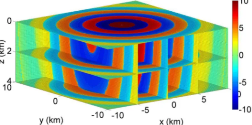
when IG is negative. The diffusive field from a point-source is shown in Figure 2.2. All the
Figure 2.2: The point-source 3D scalar diffusive field log-transformed with the source at (0,0,0).
approximate diffusivity of an electromagnetic wave in seawater (Fan et al., 2010). Figure 2.2 demonstrates how the field excited by a single point source diffuses through a 3D volume; the strength of the field decreases with increasing depth. We then apply synthetic aperture to the 2D source distribution in the inline and crossline directions. The unsteered field depicted in Figure 2.3 has five synthetic aperture sources each 5 km long. The sources in the five lines are summed, without any phase shifts and amplitude factors applied, in the x- and y-directions to produce a larger, longer source.
Figure 2.3: The unsteered 3D scalar diffusive field log-transformed.
In CSEM the longest source dipole is around 300 meters (Constable, 2010); with synthetic aperture, we can create a much longer source without requiring a boat to tow the extra-long source. Beamforming is applied to the field to change the direction of the energy. For inline steering, individual sources in each of the five lines are multiplied by a phase shift and an energy compensation term and then the sources are summed. The inline direction has more sources to use because the source is towed in the x-direction with samples taken every 100 meters. Figure 2.4 demonstrates how steering caused the field to be asymmetric towards negative x-values. The diffusive field is steered in the crossline direction much the same way as in the inline direction, but a different phase shift is applied to each synthetic aperture source with all the individual sources on one line multiplied by the same phase shift. As shown in Figure 2.5, this produces an asymmetric movement of the strength of the field in the negative y-direction. It is promising that even with five lines spaced 2km apart, we can
Figure 2.4: The 3D scalar diffusive field log-transformed and steered at a 45◦ angle in the inline direction. The arrow shows the shift in the x-direction of the energy from the origin; without steering the maximum energy would be located at the center of the source lines (x= 0km).
achieve a marked crossline steering of the field; the maximum of the field has been shifted to the right, away from the centerline of the survey (y = 0km). This leads us to believe that once applied to CSEM, crossline steering may direct the field toward a target. Inline and crossline steering can be combined to create a field that has energy shifted in the x-and y-directions (Figure 2.6). The combined steering creates a field that is asymmetric with respect to both axes, concentrating the energy in on area.
Figure 2.5: The 3D scalar diffusive field log-transformed and steered at a 45◦ angle in the crossline direction. The arrow shows the shift in the energy from the centerline of the survey (y= 0km). The shift is less than in Figure 2.4 because fewer sources are used.
Applying synthetic aperture to diffusive fields demonstrates the possibilities of using 3D synthetic aperture on real electromagnetic fields acquired from CSEM surveys. The inline
Figure 2.6: The 3D scalar diffusive field log-transformed and steered at a 45◦ angle in the inline and crossline directions. The arrows demonstrate the shift in the energy in the x- and y- directions.
and crossline steering of diffusive fields shows how the maximum can be shifted to a new area, which allows that area to be illuminated than without steering. The log-transform is a useful tool to view diffusive fields but it has some drawbacks. The only information communicated is the sign and normalized amplitude of the field. There is no information about the direction of the field or a sense of how it propagates in 3D space. We developed a new way to visualize the fields that shows the direction and propagation of the fields in the frequency-domain.
2.4 3D Visualization
The most common way to visualize electric and magnetic fields is through magnitude and phase plots but these lack the capability to show the direction the field is traveling (Constable, 2010). Additionally, the log-transformation employed in the previous figures only shows the sign and normalized amplitude of the field, but we need to visualize the direction of the field to identify the enhancement of the upgoing field from synthetic aperture and beamforming because the most important information from a CSEM survey is the electromagnetic signal that propagates down, through the reservoir, and then returns to the seafloor to be recorded by a receiver. This signal is difficult to identify because it is much weaker compared to the background field. The Poynting vector measures the direction in which the energy flux of the electromagnetic field is traveling; it is an effective way to examine how an electromagnetic
field propagates (Fan et al., 2012). The energy flux density of the electromagnetic field is given by (Griffiths, 2008)
S ≡ 1 µo
E × B, (2.9)
where µo is the permeability of free space, E, is the electric field, and B is the magnetic
field. The diffusive field, an approximation of a diffusive electric field, we use is a scalar field and therefore the Poynting vector cannot be used. The gradient of a scalar field is, however, similar to the Poynting vector for an electromagnetic field: the Poynting vector is the energy flux density of the electromagnetic field which is similar to the heat flux density used in thermodynamics. The heat flux density is found by taking the gradient of temperature, which makes the gradient a useful measure of the energy flux for scalar diffusive fields (Schroeder, 1999). The gradient of a diffusive field is complex and only the real part is used to display the gradient, normalized to make the direction apparent. In addition to visualizing the direction of the field, it is useful to know the direction of the field in relation to the time over which the field has propagated; the use of the phase of the field in conjunction with the gradient allows a frequency-domain field to appear to propagate through time. A simple example demonstrates this concept. Consider a point-source field, eikr where k is the wavenumber
and r is the distance from the source to another location in space. In that case, the phase is, then, equal to kr which smoothly increases with respect to r. A small phase corresponds to a location close to the source and a large phase corresponds to a location farther away from the source. Thus, when the phase is binned by multiplies of π the frequency-domain diffusive field appears to propagate outward in space the same way it propagates through time. The phase must not contain phase-jumps for use in our visualization method. To make the phase of the field increase smoothly, we use unwrapping in 3D which corrects the phase-jumps of 2π that occur in the field. Phase unwrapping is applied in many fields including radar, medical, and geophysics; 3D phase unwrapping is an ongoing field of research (Itoh, 1982; Parkhurst et al., 2011; Shanker & Zebker, 2010; Wang et al., 2011). Phase unwrapping is simple for our noiseless scalar diffusive fields; we unwrap the phase one dimension at a
time to construct a smoothly increasing phase. Phase jumps determined to be larger than the tolerance value π are reduced by adding or subtracting 2π to until the jump is less than the tolerance value. Once the phase is unwrapped, we add a constant to the phase field to make the source phase equal to zero. Only the relative phase is needed to view a scalar diffusive field with this method. The source is time-varying with a period of four seconds, which creates a change in the direction of the field; to show only one type of direction on the image, the phase is binned by multiples of π. The gradient that corresponds to each phase bin is shown consecutively; as the phase increases the gradient is displayed at an increasing distance from the source.
2.4.1 Numerical Examples
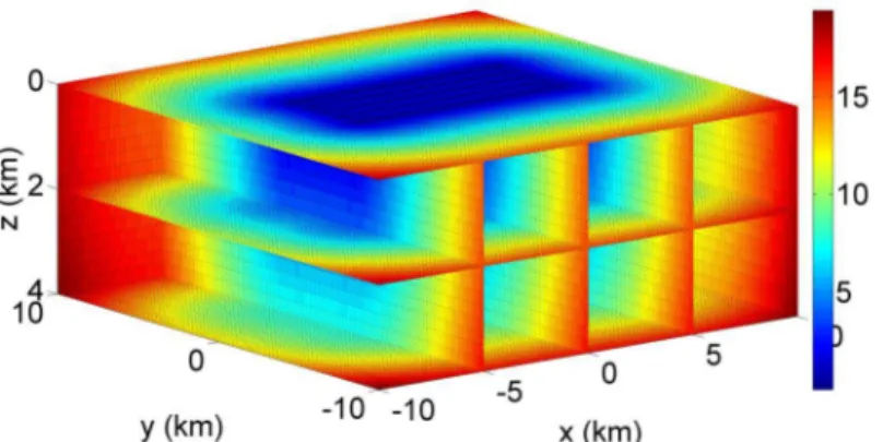
As in the previous section, the volume of the diffusive field is 20km×20km×4km to represent a CSEM survey area. We first demonstrate the phase-binned gradient visualization technique with a simple point-source before applying the method to a field with a synthetic aperture source. The phase and gradient are shown in Figure 2.7 and Figure 2.8 to compare with the 3D phase-binned gradient in Figure 2.9.
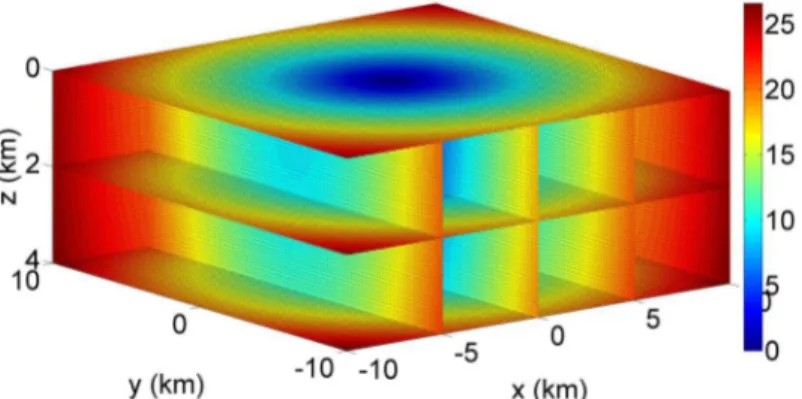
Figure 2.7: The unwrapped phase of a scalar diffusive field from a point-source located at (0,0,0). The colorbar displays radians.
The temporal evolution of the field cannot be viewed with the gradient or the phase. The advantage of the phase-binned gradient is that it displays the direction of the energy from
Figure 2.8: The normalized gradient of a scalar diffusive field from a point-source location at (0,0,0).
Figure 2.9: The phase-binned gradient of a scalar diffusive field from a point-source located at (0,0,0). The change in direction occurs from the time-harmonic point-source.
the origin outward to the edges of the model as a function of increasing phase. The direction of the field is displayed for different phase bins; a smaller phase corresponds to parts of the field closer to the source and a larger phase corresponds to parts of the field farther away from the source. This type of visualization becomes more useful when examining a field with synthetic aperture and steering, which are more complex than the point-source example. Figure 2.10 and Figure 2.11 display the unwrapped phase and gradient, respectively, of a scalar diffusive field with five 5km synthetic aperture sources.
Figure 2.10: The unwrapped phase of a scalar diffusive field with five lines of synthetic aperture sources. The colorbar displays radians.
Figure 2.11: The normalized gradient of a scalar diffusive field with five synthetic aperture sources.
The phase of the unsteered diffusive field (Figure 2.10) created from synthetic aperture sources displays the change to a 2D source distribution when compared with the phase
of the point-source (Figure 2.7). However, it does not show the change in the direction as a result of the application of synthetic aperture because no steering is applied to this example. The gradient of the unsteered diffusive field, Figure 2.11, does display the direction of the field but it is difficult to see the differences between the unsteered synthetic aperture source and the point-source gradient, shown in Figure 2.8. The phase-binned gradient of the unsteered diffusive field allows the differences to be highlighted. Figure 2.12, in comparison to Figure 2.9, demonstrates the effect of synthetic aperture through the broadening of the pattern of arrows depicted in each phase, a result of the 2D distribution of the synthetic aperture source.
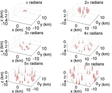
Figure 2.12: The phase-binned gradient of a scalar diffusive field with five unsteered syn-thetic aperture sources. The movement of the energy is symmetric about both the x and y directions.
The inline and crossline phase-binned gradient plots (Figure 2.13 and Figure 2.14) demon-strate how the direction of energy propagation changes with the use of beamforming. The inline field, shown in Figure 2.13, is steered at a 45◦ angle in the inline direction which causes constructive interference to occur at large x values compared to the unsteered field in
Fig-ure 2.12, which has the same amount of energy at all values of x. The interference is difficult to view with the log-transform, as previously shown in Figure 2.4, because the amplitude of the energy is small in the area 45◦ from the x-axis. The crossline field is steered at 45◦
Figure 2.13: The phase-binned gradient of a scalar diffusive field with five synthetic aperture sources steered in the inline direction at a 45◦. The energy is moving asymmetrically in the x-direction unlike the symmetric movement of the unsteered field.
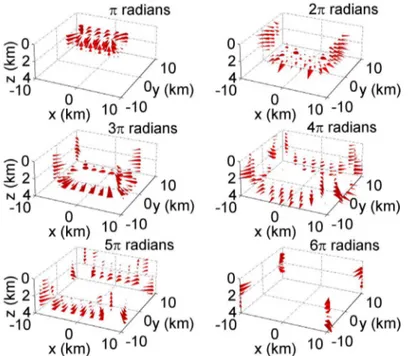
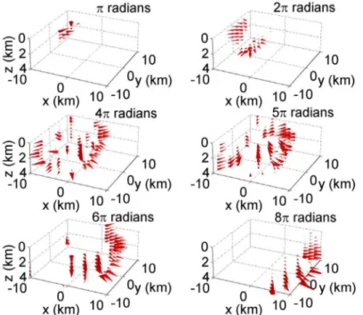
which is visible in the lower right panels of Figure 2.14 as a preferential propagation in the crossline direction (large values of y). Rather than staying symmetric about the y-axis, the crossline steering causes the interference to occur at large y values in late phases. As with the inline field, this is difficult to visualize without the phase-binned display of the direction of propagation. The combination of inline and crossline steering produces a diffusive field with energy in one area of the model. In Figure 2.15, the concentration of energy to large x and y values is displayed in the later phases of the field. Without the phase-binned gradient technique the change in the direction due to beamforming is nearly impossible to visualize, especially with in a 3D volume. Figure 2.16 depicts an y-z view of the unsteered diffusive field gradient and the combined inline and crossline steered diffusive field gradient. The oval
Figure 2.14: The phase-binned gradient of a scalar diffusive field with five synthetic aperture sources steered in the crossline direction at 45◦. The energy is moving asymmetrically in the negative y-direction in contrast to the symmetric movement of the unsteered field.
Figure 2.15: The phase-binned gradient of a scalar diffusive field steered in the inline and crossline directions at 45◦. The combined inline and crossline steering produces a field whose energy moves out asymmetrically in both the x- and y-directions.
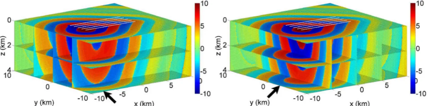
Figure 2.16: The y-z view of the unsteered diffusive field, panel a), and the combined inline and crossline steered diffusive field, panel b), at a phase of 3π. The oval highlights the change in the direction of the field caused by steering.
shape highlights the change in the direction of the field cause by steering. The unsteered field, panel a) of Figure 2.16, has mostly horizontal arrows. When steering is performed, panel b) of Figure 2.16, the arrows change to have an increased upward direction. CSEM measurements are effective for detecting reservoirs when the field propagates in the near vertical directions. Figure 2.16 demonstrates that with a diffusive field steering can modify the direction the energy propagates.
The differences in the direction of the diffusive fields can be used to determine if the synthetic aperture is steered optimally for a specific example. For CSEM fields, where the Poynting vectors are used instead of the gradient the goal is to increase the amount of upgoing energy that carries information about the reservoir. This visualization method will identify how the field propagates and how to optimize the beamforming parameters.
2.5 Discussion and Conclusions
The synthetic aperture technique offers a way to address some of the limitations of CSEM without requiring any changes in acquisition. Applying the technique to diffusive fields with 2D source distributions demonstrates the possibilities the technique has to increase the detectability of hydrocarbon reservoirs with CSEM fields. Steering the fields in both the inline and crossline directions causes the strength of the field to move to a localized area. Research is ongoing to apply this technique to synthetic CSEM fields to quantify the benefits of steering with a 2D source. The new visualization technique we introduce demonstrates how a frequency-domain field can appear to propagate as a function of increasing phase. The combined phase and gradient (or Poynting vector) provide a way to visualize how the steering modifies the upgoing field so that amount of information about the target is maximized. This is an improvement over other visualization methods that only show the amplitude or sign of the field. The implementation of these techniques increases the amount of information gleaned from data acquired from the CSEM survey, making CSEM a more valuable tool for industry. The next step is to apply the methods to electromagnetic fields with reservoirs. We will investigate what type of acquisition geometry maximizes the benefits of steering with synthetic aperture and how to optimize the steering.
2.6 Acknowledgments
We thank the Shell EM Research Team, especially Liam ´O S´uilleabh´ain, Mark Rosen-quist, Yuanzhong Fan, and David Ramirez-Mejia, for research suggestions and industry perspective. We are grateful for the financial support from the Shell Gamechanger Program of Shell Research, and thank Shell Research for the permission to publish this work.
CHAPTER 3
3D SYNTHETIC APERTURE FOR CSEM
Allison Knaak,1 Roel Snieder,1 Yuanzhong Fan,2 and David Ramirez-Mejia2
Published in The Leading Edge (2013): 32, 972-978 3.1 Abstract
Controlled-source electromagnetics (CSEM) is a geophysical electromagnetic method used to detect hydrocarbon reservoirs in marine settings. Used mainly as a derisking tool by the industry, the applicability of CSEM is limited by the size of the target, low-spatial resolution, and depth of the reservoir. Synthetic aperture, a technique that increases the size of the source by combining multiple individual sources, has been applied to CSEM fields to increase the detectability of hydrocarbon reservoirs. We apply synthetic aperture to a 3D synthetic CSEM field with a 2D source distribution to evaluate the benefits of the technique. The 2D source allows steering in the inline and crossline directions. We present an optimized beamforming of the 2D source, which increases the detectability of the reservoir. With only a portion of three towlines spaced 2 km apart, we enhance the anomaly from the target by 80%. We also demonstrate the benefits of using the Poynting vector to view CSEM fields in 3D. Synthetic aperture, beamforming, and Poynting vectors are tools that will increase the amount of information gained from CSEM survey data.
3.2 Introduction
Controlled-source electromagnetics (CSEM) is a geophysical electromagnetic method used for detecting hydrocarbon reservoirs in marine settings. First developed in academia in the 1970s, a CSEM survey involves towing a horizontal antenna just above the seafloor, where electromagnetic receivers are placed. The oil industry has used CSEM for almost two
1Center for Wave Phenomena, Colorado School of Mines, Golden, CO 2Shell International Exploration & Production, Houston, TX
decades as a derisking tool in the exploration of hydrocarbon reservoirs (Constable, 2010; Constable & Srnka, 2007; Edwards, 2005). CSEM is often used in conjunction with other geophysical methods such as seismic but it has limitations that prevent it from gaining more widespread use in industry. The limitations come from the fact that the electromagnetic field in CSEM is a predominantly diffusive field. For the reservoir to be detectable, the lateral extent of the reservoir must be large enough compared to the depth of burial, and enough of the weak signal from the reservoir must reach the receivers (Constable & Srnka, 2007; Fan et al., 2010). Also compared to seismic methods, the spatial resolution of CSEM is low (Constable, 2010).
These drawbacks prompted an investigation of how to improve the signal received from the reservoir through synthetic aperture, a method developed for radar and sonar that con-structs a larger virtual source by using the interference of fields created by different sources (Barber, 1985; Bellettini & Pinto, 2002). Fan et al. (2010) demonstrate for a 1D array of sources that the wave-based concept of synthetic aperture sources can also be applied to CSEM fields and that it can be used to improve the detectability of reservoirs. The similar-ities in the frequency-domain expressions of diffusive and wave fields show that a diffusive field at a single frequency does have a specific direction of propagation (Fan et al., 2010). Synthetic aperture allows for the use of beamforming, a technique used to create a directional transmission from a source or sensor array (see Van Veen & Buckley, 1988). One can apply the basic principles of phase shifts and addition to electromagnetic fields to change the direc-tion in which the energy moves. The shifts create constructive and destructive interference between the energy propagating in the field that, with a CSEM field, can increase the illumi-nation of the reservoir (Fan et al., 2012). Manipulating diffusive fields by using interference is not necessarily new; physicists have previously used the interference of diffusive fields for a variety of applications (Wang & Mandelis, 1999; Yodh & Chance, 1995). Fan et al. (2010) applied the concepts of synthetic aperture and beamforming to CSEM fields with one line of sources. They demonstrated the advantages of synthetic aperture steering and focusing to