Air flow over roughness discontinuity

July 1970

AIR FLOW OVER ROUGHNESS DISCONTINUITY

by Fei-Fan Yeh

and

E. C. Nickerson

Prepared Under Office of Naval Research Contract No. NOOOl4-68-A-0493-000l Project No. NR 062-4l4/6-6-68(Code 438)

U.S. Department of Defense Washington, D. C.

"This document has been approved for public release and sale; its distribution is unlimited."

Fluid Dynamics and Diffusion Laboratory College of Engineering

Colorado State University Fort Collins, Colorado

111111111111101

U18'101 057571'1 CER70-71FFY-ECN6

AIR FLOW OVER ROUGHNESS DISCONTINUITY

Measurements of mean velocity, mean-square turbulent velocity, turbulent shear stress, one-dimensional spectrum, and mass concentra-tion distribuconcentra-tions following a step increase in surface roughness of a wind-tunnel boundary-layer flow are presented. The mean velocity distributions agree well with Nickerson's (1968) numerical calcula-tions for a small roughness change. The mixing-length distribution in the "transitory" region is not experimentally consistent with that established for fully-developed turbulent boundary layer. Turbulent intensity and shear stress are generated progressively towards the upper layer as one moves downstream from the roughness discontinuity. The high frequency end of the spectra in the "transitory" region can be exactly represented by the high frequency shape of the undisturbed turbulent boundary layer. Self-preserving mass concentration profiles are in general possible for both the vertical and horizontal distribu-tions. The adjustment of the mean motion to the roughness change is more rapid than that of the turbulence.

Olapter I II LIST OF TABLES • • LIST OF FIGURES

.

.

.

LIST OF SYMBOLS INTRODUCTION • • •

. . .

.

nmORETICAL AND EXPERIMENTAL BACKGROUND 2.1

2.2

Statement of the Problem • • • • • 2.1.1 Basic equations • • • • • • • •

2.1.2 Possibility of wall variable similarity •• 2.1.3 The effect of rouglmess change

on turbulence • • • • • Literature Review • • • • • •

2.2.1 Clauser'S qualitative argument • • • • • • 2.2.2 Theories of internal boundary layer

2.2.3 Numerical simulation • • • • • • 2.2.4 Laboratory simulations and field

observations • • • • • • • • • • •

.

..

2.2.5 Review of the related diffusion studies ••

v vi ix 1 3 3 3 6 8 10 10 11 16 19 20 III EXPERIMENTAL EQUIPMENT AND MEASUREMENT PROCEDURE • .. • 23

IV

3.1 Wind Tunnel and Equipments for the Flow Setup 23 3.2 Measurements of Mean Velocity and Pressure

Gradient. • • • • • • • • • • • • • • • 25 3.3 Measurements of Turbulence • • • • • • • • • • • 26

3.3.1 Hot-wire anemometer and associated

instrumentations • • • • • • • • • 26 3.3.2 Calculations of turbulent intensities

and shear stress • • . • • • 28 3.4 Measurements of Mass Concentration 30 RESULTS AND DISSCUSSION

4.1 Description of the Results • • • • 4.1.1 Mean velocity distributions and

streamlines • . . • . • • • • 4.1.2 Mean velocity structure of internal

boundary 1 ayer • • • • 4.1.3 Turbulent results • • • 4.1.4 Momentum transfer • • • • 4.1.5 Mass diffusion results

iii 32 33 33 3S 40 44 46

Chapter

v

4.2 Application of Results to Theoretical Models • . • . • . • • • . . • • . •

4.2.1 DevelopDlent of internal boundary layer. 4.2.2 Mean velocity distributions compared

wi th Nickerson I s model •• CONCLUSIONS • • • • • • •

5.1 Mean Velocity Field 5.2 Turbulence Field • 5.3 Mass Transfer REFERENCES • . • .

APPENDIX I • • • • • • • • APPENDIX II - Tables

APPENDIX III - Figures

iv 49 49 52 54 54 55 55 57 62 66 81

Table I II III IV V VI VII VIII

Mean Velocity Data for Case I • • . Mean Velocity Data for Case II •• Mean Velocity Data for Case III

*

0, 0 ,

a,

U* and z for All Cases. o

(a) (b)

U2, W2

and -uw Data for Case I. •

V2

Data for Case I • • . (c)

-uw

Data for Case II.

Data on One-Dimensional Spectra for Case I

Parameters Used in Spectral Calculations for Case I Mass Diffusion Data for Case I • • . . • • • • • • .

v 67 68 69 70 71 72 72 73 77 78

Figure 1 2 3 4 5 6 7 8 9 10 11

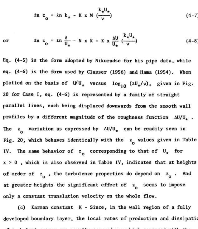
Coordinate system and flow features Plan view of wind tunnel . • . • . Flat plate and pressure taps . . Non-dimensional plot of wall pressure distributions on the flat plate •

Mean velocity distributions at x

=

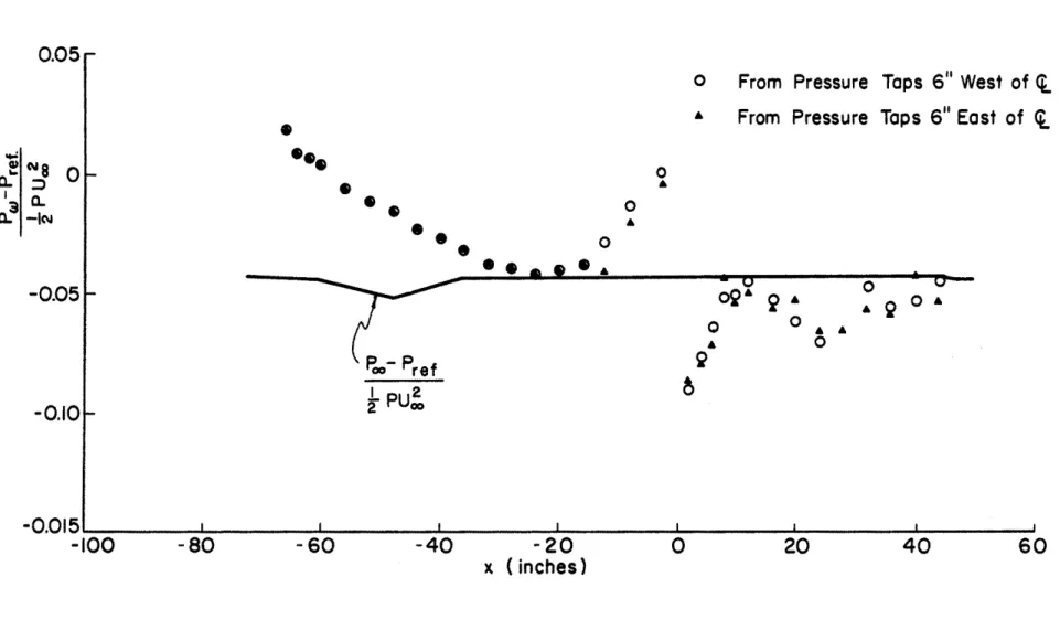
3 ft to check the two-dimensionality of the flow . •

U 2 distributions at x = 3 ft to check the two-dimensionality of the flow Test section geometry . .

False wind tunnel ceiling to obtain zero pressure gradient over flat plate • Non-dimensional plot of static pressure distribution at the free stream along the flat plate (p _re f = wall pressure at

x

= -

3 ft) . . . . Comparison of mean velocity distributions measured by the hot wire and the pitot tube at x = 2 in. . . • . . Rlock diagram for turbulence measurements 12 Coordinates of the single and the crossed

13 14 15 16 17 hot wires .

Mean velocity, streamline and -uw butions in the x-z plane for Case I

distri-Mean velocity and streamline distributions in the x-z plane for Cases II and III . Longitudinal velocity distributions for Case I.

.

_·

_·

_·

_{· ·}

_·

_·

_·

_·

_·

_{· · ·}

_·

Longitudinal velocity distributions for Case II

.

_·

_·

_{· · · ·}

_{· ·}

_{· ·}

_·

Longitudinal velocity distributions for Case III.

_{· ·}

_·

_·

_·

_{· ·}

_·

_{· ·}

_·

_·

_·

_·

vi

·

·

·

82 83 84 85 86 87 88 89 90 91 92 93 94 95

· · .

_·

·

·

96

· · . · · ·

97

· ·

·

·

·

98

Figure 18

19 20

A semi-log plot of non-dimensional velocity distributions for Case I . .

Shear velocity distributions for Case I

zU

U/U* vs. loglO ( v*) for Case I . • • . • 21 Karman constant and wall pressure

22 23 24 25 26 27 28 29 30 31 32 33 34

measurements for Case I.

Karman constant and wall pressure measurements for Case II . . • • •

uz,

V2,

and

W2

Case I •

distributions for

Normalized spectra of longitudinal velocity fluctuations at x

= -

12 in. for Case I • • Normalized spectra of longitudinal velocity fluctuations at x = 4 in. for Case I

Normalized spectra of longitudinal velocity fluctuations at x

=

6 in. for Case I

Normalized spectra of longitudinal velocity fluctuations at x

=

12 in. for Case I • u'-spectra in the similarity coordinates at x

= -

12 in. for Case I . . • • • • u'-spectra in the similarity coordinates at x

=

4 in. for Case I • • • • • • • • u'-spectra in the similarity coordinates at x = 6 in. for Case I . . • • . • • • u'-spectra in the similarity coordinates at x = 12 in. for Case I . . . • Distributions of the vertical turbulent diffusivity for Case I . . . .

Distributions of the mixing length for Case I . . . .

Distributions of a_l

=

T -2 Pq and x

=

6 in. for Case I . .

vii at

x

=

4 in. 99 100 101 102 103 104 105 106 107 108 109 110 111 112 113 114 115

Figure

35

36

(T/p)3/2

Non-dimensional distributions of L

=

~~~--at x

=

4 in. and x

=

6 in. for Case I .

~

. . . 116 (q2 3/2

Non-dimens~onal distribut~ons

of

LE

=

q

~

at x

=

4 In. and x

=

6 In. for CaSe I . . . 117

37 Typical profiles of the vertical mass

concentra-tion for Case I . . . • . . . 118

38 Typical profiles of the horizontal mass

concentra-tion for Case I . . . . . . . . 119

39 Non-dimensional plot of the vertical

concentra-tion profiles . . . . . . . . . . . 120 40 Non-dimensional plot of the horizontal

concen-tration profiles . . . 121

41 Decrease of C with

x

for Case I . . . 122 max

42 Growth of A and n with x for Case I . 123

43 Growth of the surface of the internal boundary

layer, compared with that of the critical surface . . . • 124 44 Non-dimensional plot of the velocity defect law

for Case I. . . . . . . . 125 45 Mean velocity distributions for Case I compared

with Nickerson's model . . . 126 46 Mean velocity distributions for Case II compared

with Nickerson's model . . . 127

47 Mean velocity distributions for Case III

compared with Nickerson's model . . . . • . . . 128

Symbol A(z) a C c D .• 1J D ,D ,D

x Y z

d(x) E(k) F(k l)

F(~), f(~)

f G H Definition Constant

Change of velocity due to the flow acceleration

Constant

Empirical fUnction as defined in Eq. (2-32)

Constant Constant

Mass concentration

Maximum mass concentration Constant

Eddy diffusivity tensor Eddy diffusivities in x,y,z directions

Thickness of the internal bOWldary layer

Mean voltage output across the hot wire

Three-dimensional energy spectrum f1.Dlction

Fluctuating voltage across the hot wire

One-dimensional spectrum fWlction Universal function

Frequency

Empirical function as defined in Eq. (2-34) Ratio of ~+ to

a

ix Dimension ppm ppm L L L -1 T

Symbol I(t) K k L M m N n p R •• 1.J t U,V,W Definition

An impulse input function

K8.r.m8n

Constant

Three-dimensional wave number One-dimensional wave number Kolmogorov's wave number

A roughness characteristic length

Dimension -1 L -1 L -1 L L

Stability length, also defined as in eq. (2-33) L Mixing-length components in x,y,z

directions Nondimensional function Constant Nondimensional function Constant Mean pressure Reference pressure

Strength of a continuous point source

Total turbulent kinetic energy per unit mass

Velocity correlation function Time

Mean velocity components in x,y,z directions

Free-stream velocity Shear velocity

Shear velocity downwind of the roughness discontinuity x L ML -IT-2 ML- IT-2 ML- 3

Symbol u,v,w x,y,z x _s z a(-) L y 0*

o

(z) £ 6 Definition

Shear velocity upwind of the roughness discontinuity

Velocity fluctuations in x,y,z directions

Distance along longitudinal, lateral and vertical direction

Coordinate of x axis of the diffusion source

Heights

Roughness length downwind of the roughness discontinuity

Roughness length upwind of the roughness discontinuity

Constant

A dimensionless function Angle of velocity vector Exponential constant Boundary layer thickness Displacement thickness

A characteristic thickness Change of velocity due to the streamline displacement

Angle deviation of hot wire Turbulent energy dissipation Momentum thickness

Angle of hot wire to velocity vector One-half of the plume-spreading width, at which the local mass concentration is one-half of the value at ground level

xi Dimension L L L L L L L L L

Symbol A (x) p a .. 1J

,

..

1J Definition

Height at which the local mass concentration is one-half of the value at ground level

Coefficient of dynamic viscosity Mean mass density of the air Mass diffusivity tensor Mass diffusivity in x,y,z direction

Shear stress Wall shear stress Maximum shear stress Energy spectrum function Dimensional stream function

xii Dimension L L2T- I ML-3 L2T- I L2T- I ML- IT-2 ML-IT-2 ML-IT-2 L3T- 2 L2T- I

INTRODUCTION

The surface layer in the lower 1000 meters of the atmosphere over a homogeneous terrain has been extensively investigated and successfully simulated by the boundary layer along a flat plate in wind tunnels. In reality, however, homogeneous terrain exists only over a limited area. Ver.l little is known about the effect of surface non-homogeneity on boundary layer flOWS, and neither wind-ttmnel data nor field data are available in sufficient quantity to deduce a general analytical model.

The effect of an abrupt increase in surface roughness is felt in the turbulent wind field downstream in two ways: a modified mean flow pattern develops according to the theory of the internal boundary layer

(Elliott, 1958) and a "disturbed" turbulence mechanism is set into action whiCh later is responsible for returning the flow to another relaxed state. Therefore, the existing semi-empirical models based on the present knowledge of so-called "pure" turbulence in calculating the mean flow distribution are highly questionable. Among many of the

theoretical investigators the self-preservation approaCh of Townsend (1965a, 1965b, 1966) is certainly useful but still requires some assumptions about the interaction between the velocity field and the turbulent motion, in order to give quantitative results. The main requirement at this stage would appear to be an accurate and compre-hensive experimental study of these flows whiCh will perhaps throw

further light on the mechanism involved.

(1) to investigate systematically the mean flow field upstream and downstream from the roughness discontinuity and to compare the existing theories with the experiments;

(2) to study the turbulence structure of the internal boundary layer by means of extensive hot-wire surveys, and

(3) to measure the spread of diffusing matter and compare the spread rate with that obtained in a fully developed boundary layer over homogeneous terrain, since the effect of roughness discontinuity could cause significant difference in the convective force of the mean motion and the rate of eddy flux.

And finally, the suggested means of improving existing theories will be outlined.

It is also felt that the present investigation might, enhance the understanding of general boundary layer turbulence, since the turbulence mechanism could only be closely observed when its asymptotic state is perturbed (Clauser, 1956).

Chapter II

nmORETICAL AND EXPERIMENTAL BACKGROUND

The historical development of the calculation of internal boundary layers is characterized by the fact that the system of equations govern-ing turbulent flow is not closed. Thus" solutions to the problem can only be obtained with the aid of empirical and hypothetical relation-ships. Since the results established to date are not fully satisfactory, many different approaches to the prob lem have been advanced. In this chapter, a comprehensive discussion of this problem in connection with the present experiment will be stated, and a summary of existing theo-retical models, as well as most of the related measurements, will be given.

2.1 Statement of the Problem

2.1.1 Basic equations - Let us consider a steady, two-dimensional, turbulent boundary layer in neutral hydrostatic stability. Only the case of the flow moving from the aerodynamically smooth to the aerody-namically rough with negligible pressure gradient outside of the layer is treated. All the physical interpretations of the results should also be applicable to flows for which the aerodynamic roughness changes from

rough to smooth.

As an introduction to the more general problem, the roughness is homogeneously distributed over the rough surface, but the corresponding

roughness length z is not necessarily small in comparison with the o

boundary layer thickness is extremely large compared with the step change in the characteristic roughness dimension, i.e., the condition

Z «<5

is not necessarily satisfied. Such a condition would possibly be

satisfied in the atmospheric boundary layer for small roughness heights, but would be extremely unfeasible in the laboratory for perhaps an

immeasurab Ie change in roughness.

The approaching turbulent boundary layer over the smooth surface is assumed to be fully developed so that a universal quasi-stationary state is reached and certain siDli1 ari ty profiles are attained. The step increase of surface roughness will serve to perturb this asymptotic state, and as this results, the flow in the region immediately downstream

(and very likely upstream) of the roughness discontinuity will be in a "transitory" state before relaxing to a new asymptotic state. The pres-ent investigation will concpres-entrate on the developmpres-ent of the turbulpres-ent botmdary layer in this "transitory" region.

A Cartesian coordinate system (Fig. 1) is used in which U,V,W

denote the components of the mean velocity, and u, v,w the corresponding fluctuations in x,y,z directions. The Navier-Stokes equations in the x-z plane, after averaging in the y direction, reduce to

(2-2)

(2-3)

in which the ordinary viscous terms are negligible in comparison with the eddy stress tems except in the wall region. Together with the continuity equation

au

+

aw

=

0

they fom the basic system of equations that must be solved. The

closure of the system of equations in solving for U,W, and p requires that all the statistical quantities of turbulence be specified. The b01.Uldary conditions to which this system is subjected can be readily prescribed in the usual sense of b01.Uldary layer calculations.

A

closure of the system of equations in the light of analogy with "mixing-length" hypothesis can be formulated, if it is assumed that the components of turbulent flux tensor relative to the axes oxyz are related in a simple homogeneous linear fashion to the gradient of mean velocity vector, i.e., - u.u. 1 ) = (DT)· . 1)

[

au

i

au.]

-+~ ax. ax. ) 1 (2-5)

in which the second order tensor (D

T).. 1) is, in general, a f1.Ulction of

position (not of time) since the relation between -u.u.

1 ) and

[

au. au.l

~ + ~! will be defined at every point of the flow field.

oX_j oX i

J

Physi-cally, (D

T).. must be strictly a property of the turbulent motion, and 1)

we should not here complicate the analysis to discuss the fourth-order (D

T) .. as Hinze (1959) pointed out. For two-dimensional flow, Eq. 1) (2-5)

becomes

( -U2

[xx

D 2 au au aw -uw \

,

(

- +

ax)

\ XZ\ ax az I

=

I I

-WL

J

j

au aw 2 aw -uw D - + zx zz az ax az (2-6) in which ( Dxx

:xz)

( -uix -Uiz

1

=

Dzx _zz -wt -wt J x z (2-7)

and~ in turn~ R.

x and R.z are the components of a hypothetically

-+

vectorial mixing-length R. in the x and z directions. Thus ~ the solu-tion of the basic equasolu-tions requires the informasolu-tion of three empirical problems; that is~ certain factors must be fotmd:

(1) Whether or not w is of the same order of magnitude as u~ such that

i-wi

I

= const xl-uR.

I

and l-wR.

I

=

const xi-oR.

I

can be

x x z z

used as in mixing-length theory.

(2) Whether or not the eddy coefficient -01 ~ which governs the

z

vertical mixing~ can aSS1.De a functional form of the Wall law as a lower boundary condition in the "transitory region".

(3) Whether the order of magnitude of -01 ~ which governs the z

horizontal mixing~ can be estimated, as well as its role in solving the basic equations.

2.1.2 Possibility of wall variable similarity - Based on the above-mentioned resolution difficulties~ the similarity arg1.Dents will naturally

lead us to examine the experimental data in the context of the fUnctional hypotheses of Clauser (1956) and Coles (1956).

Near the surface but outside the viscous sublayer, the only important length variable for the mean motion is the normal distance from the wall z, and the only important velocity scale is U*

=

(Tw/p)1/2

~

thus, immediately, by the dimensional argument,

(2-8)

in which K is the Karman's constant, known to be approximately 0.4 in the wall region of the fully developed turbulent botmdary layer. Whether K should be a constant or not in the "transitory" region is not known.

llowever, it can easily be deduced that K will at least be a function of x by introducing the vertical mean velocity component Vex) into the conventional Karman's similarity analysis, which was based on the assump-tion of a parallel flow (Schlichting, 1960), and

dU d2U K constant dz dz 2 = x dU d2W dz dx2 (2-9)

The derivation of this relation is shown in detail in Appendix I. Integration of (2-8) for a given x gives

U 1 z

I n -U* - K z

o

(2-10)

in which z _o is the characteristic roughness length of the surface, introduced as the result of integration constant.

The wind profile expressed by Eq. (2-10) has received a great deal of experimental support, but only for flows over homogeneous surfaces. Here, we would expect that both the smooth and rough surfaces should

correspondingly possess a horizontal uniform Zo except near the dis-continuity. Physically, the z should be assumed to have a rapid

o

change, but still in a certain continuous fashion over the step change of surface roughness. Thus, we have to obtain adequate knowledge con-cerning the functional form of the horizontal variation of z in order

o

to justify the similarity law existing in tr.e "transitory" region. In fact, the z _o could serve as another vital scaling parameter.

According to theoretical arguments (Rotta, 1962), the assumption of similarity of the wall flow is only justified, if it includes the

~~ double velocity correlation functions R .. (x,r,t)

1.J and spectrum functions ~

~ .. (x,k) in the direction of mean flow requires forms like

1.J

I

zU* -30

t~*

) ~~ U2 r R .. (x,r,t) = G .•

_l-;-

-

,

1.J * 1.) _, Z ~ U2 z (

z~*

kZ)

cp •• (x,k) = H ..

,

1.J _* 1.J (2-11) (2-12)

in which G .. and H .. are respectively dimensionless universal double

1.J 1.)

velocity correlation functions and spectrum functions, and k is the wave number.

Though there exists experimental evidence for a subrange near the wall within which the one-dimensional spectrum function varies in accor-dance with a theoretical prediction by Tehen (1953), it is well-known--Townsend (1961) cornments--that the turbulent motion does not scale on U* and z , and it is difficult to reconcile the experimental observa-tions without supposing that the motion at any point in the wall region consists of (i) an "active" part, which is responsible for turbulent transfer and determined by the stress distribution, and (ii) and "inac-tive" part determined by the turbulence in the outer layer. The effect of an "inactive" part is supported by measurements taken by Bradshaw

(1967b) of frequency spectra in a strongly retarded boundary layer.

A noticeable increase of dissipation of kinetic energy into heat supplied by turbulent diffusion from the outer layer was observed. Consequently, we might expect such an effect on the retarding fluid near t~e wall in the "transitory" region.

2.1.3 The effect of roughness change on turbulence - From the turbulence-energy equation (Hinze, 1959),

!!...

_dt

(g:l

₂ I

=

-il.u.

~

-

_a_

u.l~

+

~)

+ v _a_ u (aui +

~\

1 J ax. ax. 1 p 2 ax. j ax. ax. !

1 1 1 J 1 rate of change ( au. au. \ _ V _1_ + ---1. I aX_j aXiJ au. ---1. ax. 1 (2-13) of kinetic energy

=

of turbulence Convective Viscous

production + Diffusion + Work + Dissipation

- a u

it is seen that, if all the terms but u2 ax are kept unchanged, the total turbulent kinetic energy tends to be increased (at the expense of the mean flow energy), as soon as the velocity of a flow decreases

(or is retarded) in the x direction, i.e., au/ax < O. Many

theoreti-cal workers, such as Townsend (196Sa, 1965b, 1966) states that the effect of roughness change is initially restricted to an "internal boundary

layer" with thickness d(x). Far above d(x) , the streamline is displaced vertically without a charge in shape of the velocity profile. On these grounds, the following inferences may be drawn.

Upon encountering the rough surface, the fluid near the wall is retarded by the increased wall shear stress. In accordance with the continuity equation, a vertical mean velocity is created to convect the lower momentum fluid away from the wall. Since the fluid

far above the d(x) is not affected, the fluid at the height of order of d(x) must be accelerated to maintain an incompressible flow, and then retarded in the downstream direction as the d(x) grows. As a result of this retarded motion, the relative turbulent intensities tend to be increased by the negative velocity gradient in the flow direction and by the higher velocity gradient due to the presence of the lower momentum fluid. The total turbulent energy is, thus, progressively

generated outward from the wall as one moves downstream from the

roughness discontinuity.

As

a consequence, the higher turbulent shear stress will tend to reduce the velocity gradient through intense

vertical mixing, and in tum, the turbulent intensity and shear

stress would decrease farther downstream to approach another asymptotic state over the rough surface.

A thorough tmderstanding of these intrinsic turbulence mechanisms, together with their interaction with the mean flow, will largely depend on the direct measurement of the individual tenns of the turbulent energy equation in the present study.

2.2 Literature Review

In order to show the relevance for the study of the behavior of bomdary layers to roughness changes, many previous predictions will be summarized and briefly reviewed. Their limitations or the range of validity will be indicated as well.

2.2.1 Clauser's qualitative argument - A qualitative understanding of the response of a botmdary layer to a roughness change began earlier with Clauser's (1956) demonstration of his black box analogy in viewing the response of the layer to an impulse input as

I (t)

=

(.~).

dTw

T dx

w

(2-14)

in which

ot

is an appropriate thickness which expresses the effect of the shear gradient in the tmiversal scheme without dependence on wall shear stress TW. The experiment was perfonned in a constant pressure

variable (ot/T ) dT /dx experienced an impulse resembling the

w w

Dirac ftmction because of the abrupt change of TW.

Three results turned out to be of particular importance in the later development of all the theoretical models.

(i) The abrupt change of skin friction was felt immediately by the fluid nearest the wall.. It propagated rapidly through the inner layers and then more slowly through the outer layer.

(ii) Even though dT / dx was nearly zero after the

w

disturbance, the layer was in a "transitory" state for a considerable distance behind the disturbance.

(iii) A longitudinal shear gradient dTw/dx has an important influence on the behavior of turbulent layers, an influence that has not been taken into accotmt in previous work, such as Jacob (1939) ..

2.2.2 Theories of internal botmdary layer - To make the flow field in the "transitory" state analytically tractable, the effect of the roughness change is assumed to be confined to a so-called "internal botmdaty layer" of thickness d(x) within which the velocity or

shear stress profiles may be represented by an assumed fonn. The flow above the boundary d(x) is moving with the speed and shear stress that it had upwind of the roughness discontinuity. Most hypo-theses on the internal botmdary layer simplify the mathematics by requiring only that the continuity equation and the botmdary layer equation in their integral forms are satisfied, that is

and d(x) \1

=

f

o

au

- - d z _ax

f

d(X)

(u au

+

w

au )

dz

= u

2 _

u

2 ax az *0 *1 o loss of momenttml by advection

net gain of momentum

= due to vertical flux

(2-15)

(2-16)

where one assumes that below d(x) near the wall, the velocity distri-bution is given by

u*

(x,z)

U = __ 0 ___ - - In _z_

K z (2-17)

o

in which K and Zo are independent of x , U*l and U*o are the surface friction velocities upwind and downwind of the roughness discon-tinuity, respectively, and zl and Zo are the corresponding roughness lengths.

Following Elliott's initial work (1958), a number of other

investigators, including Panofsky and Townsend (1964), Townsend (1965a, 1965b), Taylor (1967), and Blom and Wartena (1969), have investigated essentially the same model with different assumptions on stress distri-bution. Elliott's (1958) model contained a physically unrealistic discontinuity in stress at the interface d(x) which was implied in his assumption that

U* (x,z) _o

=

U* (x,o) ₀ for z < d(x) (2-18) Panofsky and Townsend (1964) removed this difficulty by assuming a linear variation of stress,

and were able to derive an expression for the ratio d/x for various roughness, which was on the order of 1/10 and agreed favorably with Elliott's simple dimensional argument:

(2-20)

The interesting conclusion from both predictions at this point is that the growth of d(x) is independent of wind speed, U_m ' and

viscosity, which are usually important in the development of

a boundary layer over a flat plate. The question has also been examined from a slightly different point of view, namely, as a problem in small-scale convection. R. J. Taylor (1962) reported a ratio d/x to be 1/100-150 on his wind-tunnel experiments.

P. A. Taylor (1967), based on an application of the Karman-Pohlhausen technique (Goldstein, 1938), was able to obtain a stress distribution in the form of

(2-21)

which was later found to be less suitable than the form of Eq. (2-19), in comparison with his numerical model (1968). Townsend (1965a, 1965b) tried to summarize the previous work and introduced, in a strictly theoretical manner, a self-preserving development of the change of the velocity profile downwind of the roughness discontinuity. It appears that the desired quantities can be then found by applying similarity arguments, given only in terms of the length scale d(x) and a velocity scale U*o(x) . A brief review of this similarity theory is necessary before realizing its range of validity.

Townsend distinguished the change of the velocity profile due to flow acceleration A(z) from the change due to streamline displacement o(z) , then

(2-22)

in which U

I represents the original velocity profile, given by U*l ( )

U1

=

K

In :1 (2-23)

Using the continuity equation, it is possible to derive a relation between o(z) and A(z) . Then, Townsend assumed the following self-preserving forms for A(z) and the stress distribution T

(2-24)

(2-25)

in which f(~)

d and F(~1 are universal functions, independent of x

owing to the assumed self-preservation. Substituting Eqs. (2-24) and (2-25) into the boundary layer equation

U aU +

w

au

=

aT

ax az az (2-26)

gives an ordinary differential equation for large values:

-nf'(n)

=

F'(n) (2-27)

where n = z/d. An explicit form for fen) and F(n) can be obtained only by making an assumption about the interaction between the velocity field and the turbulent motion. Townsend employed a simple assumption, namely, the "mixing length" or "eddy viscosity" assumption, and ended up with the stress distribution:

(2-28)

For the exact form of F(n) , one must look at the energy equation. In his conclusions, Townsend also remarked the self-preserving development is possible only if IU*o/U*l' is small, and if U*o» U*l. For changes of friction velocities that are not small, the dynamics of the self-preserving flow will change slowly with x. In order to compare the laboratory results of an experiment in which air flowed from a smooth surface onto a water surface, Plate and Hidy (1967) added advection to Elliott's techniques and incorporated Townsend's analysis in a modified form, such that the result can be extended to calculate the velocity distribution for the cases in which

(i) o(z) is not negligibly small compared with d(x) , (ii) the effect of non-uniform shear at the surface must be considered, and

(iii) a pressure gradient, independent of z exists in the x direction.

Blom and Wartena (1969) corrected a minor discrepancy between Townsend's resulting velocity profile and his inner boundary condition, and further extended Townsend's theory to the case of two subsequent abrupt changes of surface roughness. By means of a numerical example, they found that the grOlvth of d (x) downwind of the second abrupt change is of the same order as that behind the first one.

In cont::lusion, it is fair to state that, because of the agreement of the results of various theoretical investigators using internal-boundary-layer theory, one finds that velocity changes are relatively insensitive to

the assmnptions on the turbulent exchange process provided the velocity profile remains logarithmic clo:;.e to the surface. And quite obviously, the internal boundary layer hypothesis can hardly go beyond tt.e bcundary layer equation (Eq. 2-26) to include more significant terms that might be relevant in the study of non-homogeneous terrain, a]~o, the interface d(x) is, by all means, an ill-defined length scale from a practical point of view.

2.2.3 Numerical simulation - Numerical integration permits inclusion of terms that are difficult to be treated by internal boundary layer

models. It should therefore lead to a broader insight into the physics of the problem.

Onishi (1966) and Wagner (1966) were the first to attempt a numerical simulation of atmospheric boundary layer flow over terrain with a rough-ness discontinuity. Their models were all based on the two-dimensional Navier-Stokes equations, Eqs. (2-2) and (2-3). With the eddy diffusivity assumption, Eqs. (2-2) and (2-3) become

au _{u aw + W au =}

₁

~

_{a (}

_D

_au)

_a

_(D

_{au )}

- + at ax ax

- p

ax + ax x ax +

az

z

az

,

(2-29) and aw _{u aw +}

_{w aw}

_{= _}

_!.

~

₊

~

_(D

_aw)

₊

~

_(D

_{aw )}

- + at ax az p az ax x ax az z az (2-30)

Both Onishi and Wagner did not consider the horizontal mixing terms because D _x is not theoretically given. However, Wagner examined the relative magnitudes of these terms in a numerical scheme for roughness change from 1 cm to 10 cm, and showed that the difference on solutions was very small between two arbitrarily specified form:

D = 5D

x z

D = 0 and x

Onishi obtained solutions to the steady state equations and took into account the dynamic pressure force near the roughness discontinuity. He also introduced a linear variation of z instead of the step change

o

of z at the roughness discontinuity. Wagner's model was designed o

for an initial-value problem in an unsteady state. The condition for computational stability in his case is

6t

~

- 2D ]

U + z

l

flx (Az)2 1

(2-31)

which was derived originally for two linearized equations with forms similar to Eqs. (2-29) and (2-30). This relation proved to be usually a good approximation for the more general non-linear equations with

variable coefficients. The condition in Eq. (2-31) can also be necessary and sufficient for convergence if the initial-value problem is properly posed, as was shown by Richtmyer (1957). At about the same time, Nicker-son (1967), followed by Taylor (1968), also applied the initial value approach to integrate numerically the boundary layer equation (Eq. 2-26). Together with the continuity equation and the "mixing-length" assumption, their results near the discontinuity were found to be significantly

larger than the predictions of internal-boundary-layer theories. It turns out that agreement can be attained if the effects of vertical motion are neglected in the numerical calculations. This discrepancy

from those of internal boundary layer theories was also supported by the results of Onishi and Wagner. There is no doubt that numerical techniques should be of great value in modeling non-uniform boundary layer flows that are beyond the scope of similarity solutions. It is

for this reason that the present wind-tunnel observations co~pared Kith the numerical results such as those obtained by Nickerson (1967) are considered more significant.

Bradshaw et ale (1966), following Townsend (1961), defined three simple empirical functions relating the turbulent intensity, diffusion, and dissipation to the shear stress profile as follows,

a l T

=

--2 pq L

₌

(T/p)3/2 ~ G

₌

(~+

}

_q2 w

)/rm:c

t

~

in whi ch

<r

=

U2

+

V2

+

WL

,

T = - puw , and ~ = v(au./ax.)2

1 J

(2-32)

(2-33)

(2-34)

so that the turbulent energy equation for a two-dimensional incompressible boundary layer,

(u - + W -a a ) - q 1 -2

ax

az

2 (2-35)

can be transformed into an equation for turbulent shear stress,

U~

_laa:p

₁

+ w~

( 3a:p

1

-T

au

(Tmpax

t

:z

(G

_~

_{J +} (T/p)3/2 0 - - +

₌

ax

az

p

az

L (2-36)

This equation, together with the mean momentum equation and the mean continuity equation for a two-dimensional flow, form a hyperbolic system with three unknowns, i.e., U, Wand T . Bradshaw et ale indicated

that the numerical integrations by the method of characteristics with preliminary choices of the three empirical functions compared favorably

with the results of conventional calculation methods over a wide range of pressure gradients. By dividing through by TIp , i t can be seen

that Eq. (2-36) is the "mixing length" equation with additional terms representing advection and diffusion. Therefore, this method should be considered as a refinement of the "mixing-length" or "eddy viscosity" assumption. Most of all, their results suggested a much closer connec-tion between the shear stress profile and the turbulent structure than between the shear stress profile and the mean velocity profile, wherever the effect of the past history of the boundary layer becomes important.

2.2.4 Laboratory simulations and field observations - The early laboratory investigation of this problem has been carried out by Jacobs (1939) and Clauser (1956) with only the measurements of mean velocity distributions. Jacobs' experiments were carried out in a fully developed channel flow. He found that the surface shear stress assumed its new value immediately downstream of the discontinuity; this was not confirmed by later experiments. In Taylor's (1962) experiments, the boundary layer was formed and changed suddenly from a rough to a smooth surface. The experimental results indicated a distribution of shear stress similar to that obtained by Jacobs but the assl~ption of a logarithmic velocity dis-tribution near the roughness discontinuity appears questionable. Logan and Jones (1963) made measurements of Reynolds stresses in the "transi-tory" region following an abrupt increase in surface roughness of a pipe. They concluded that Reynolds stresses throughout much of the "transitory" region reach values exceeding those in fully developed flow in the rough pipe, and that shear stress distributions must be knO\in for use in the calculation of velocity distributions. Later, Antonia and

square-sectioned ribs were used as roughness elements. Their limited turbulence results showed the same trend as those obtained by Logan and Jones for the pipe flow. However, their mean velocity profiles both inside and outside of the inner layer exhibited a linear trend when

t:

plotted in the form U versus Z2 _{They used the point of}

intersec-tion of the two straight lines to define the edge of the "internal bOWldary layer," which was fOWld to depend linearly on x, i.e., the

inner bOWldary layer develops in the manner of a two-dimensional wake. Observations of the velocity changes Wlder various surface condi-tions have been made by several researchers, (Lettau et al., 1962; Rider, Philip and Bradley, 1963), in the atmospheric bOWldary layer, mostly for moderate values of U*o/U*l near 0.7. Accuracy of the observations is not sufficient to lead to definite results which could be used to con-firm theoretical models.

2.2.5 Review of the related diffusion studies - The only available diffusion studies Wlder the effect of topographical change are those of Hino, (1965, 1967a, 1967b). Theoretically, Hino suggested a conventional numerical analysis of the Eulerian diffusion equation for a point source

,

(2-37)

which resulted from the assumption that the principal axes of the mass diffusivity tensor

oxyz, and the term

0 . . are oriented parallel to the coordinate system

1J

a/ax (oxx aC/ax) is negligibly small compared with the convective term

u

ac/ax. In his analysis the diffusion coefficients are assumed t~ be different functional forms of total turbulent energy at different heights,

<1 = zz <1 = zz <1 = zz Al(x - Xs)nl

(~)~

for x )n2

(~)~

for s ~ m A3(~) 2 Z for

o .::.

_{Z .::. Z 1} ~ [A + B _sin2 { _(z-zl) Iz}] ((12) 2 Z Z !-.:: [A + B sin2 { (z2- z l)/z}] ((12) 2 z z (2-38) for zl < Z .::. z2 for z2 < z (2-39)

in which and are the heights from the wall where diffusion coefficients change, x

s is the coordinate of the x axis of the source, and Al ' A2 ' ... , m, n, etc. are parameters. These assumptions are basically in agreement with the two-layer model, the theory of the internal boundary layer, but the exact forms of Eqs. (2-38) and (2-39) are open to discussion.

Yamamoto and Shimanuki, (1963), reported a numerical solution of Eq. (2-37) using the vertical diffusivity derived from mixing-length theory and an assumed lateral diffusivity of the form

z

a = a a ( )

yy zz

r

(2-40)

in which a is an unknown function of z/L , where L is the stability length introduced by Monin and Obukhov, (1954). Surprisingly, a was found to be approximately 13 under neutral-stability conditions when the calculated diffusion patterns were compared with the observations made during projects Prairie Grass and Green Glow over a homogeneous terrain.

Batchelor (1959, 1964) suggested that the statistical functions relating to the motion of a marked fluid particle possess Lagrangian similarity in the constant-stress region of a turbulent boundary layer,

in which mean velocity varies as the logarithm of wall distance z. Based on this hypothesis he was able to predict that dispersion and maximum mean concentrations are proportional to certain powers of down-stream distance x. For a continuous point source at the ground level he obtained

(2-41)

Q~ are the rate of source strength, and b and c are parameters. This prediction has been supported experimentally by numer-ous others for a fully developed boundary layer, (Cermak, 1963), but has not yet been studied in the roughness-change flow. Principally, the Lagrangian similarity hypothesis can be employed to the roughness change case as long as the assumption of a constant-stress region is justified, and the velocity profile remains logarithmic close to the surface.

However, based on the previous discussion that Zo might be a function of x in the non-homogeneous terrain, Eq. (2-41) must be modified accordingly to a different functional form of x.

Chapter III

EXPERIMENTAL EQUIPMENT AND MEASUREMENT PROCEDURE

In this chapter, the experimental equipment and measurement procedure made for this study are briefly described. The instruments used were part of the standard laboratory equipment at the Fluid Dynamics and Diffusion Laboratory of Colorado State University. Emphasis is given to the establishment of the required flow conditions and turbulence

measurements.

3.1 Wind Tunnel and Equipments for the Flow Setup

The experiments were carried out in the low-speed wind tunnel (Fig. 2) at Colorado State University. The tunnel is a closed circulat-ing type with a test length of 30 ft, and a cross-sectional area of 6 x 6 ft2. The free stream turbulence level ~/Um is kept within

~ 2% by an inlet con triction ratio of 4:1 and a damping screen. Air flow in the tunnel is driven by a constant speed-pitch-controlled fan, which can vary the wind speed from 3 fps to about 75 fps. There is no arrangement for temperature control in the tunnel.

The bulk of data were taken in a thin boundary layer (approximately 3 inches at the step change of roughness), developed over a 3 ft wide flat plate, which was elevated at a height of 2 ft from the wind tunnel floor in order to avoid the secondary motions resulting from the exces-sive loss of momentum in the corners of the tunnel. The flat plate

(Fig. 3) consisted of a smooth front section of a 6 ft length and a rough downstream section of a 4 ft length. The smooth section was made of polished aluminum. A 4-inch wide strip of sandpaper (Grid 36) was

attached across the whole width of the plate at a distance of one inch ~ the leading edge for tripping the turbulent flow and thickening the boundary layer. The rough section was JDade of plywood, lDliformly and randOllly covered with a layer of angular gravel with an average size of 1/4 in. (obtained according to A.S.T.M. Specifications of u.S.

Standard Sieve Series). Since turbulence is a statistical phenomenon, the randomly distributed roughness of irregular shape should preserve this statistical concept more favorable than any geometrically well-defined roughness.

Two rows of pressure taps with 1/32 in. in diameter holes, placed at a distance of 6 in. on either side of the centerline, were used to measure the wall static pressure along the flat plate. Little appears

to be known about the accuracy of wall pressure measurements in the

irregular rough surface, but the results indicate that the flow is nearly two-dimensional because measurements from the two lines of pressure taps are considered practically identical within the experimental errors as shown in Fig. 4. A more satisfactory way fOr testing two-dimensionality of the flow should be J perhaps J perfomed by measuring the wall shear

stress pattern. The usual devices, such as Preston tubes, or even a visualization technique, were found to be very lDlcertain in application to the rough surface. Instead, a comparison of similar profiles of mean velocity and turbulent intensity

U2

within the flow extending to 8 in. on either side of the centerline for a downstream distance of 9 ft. from the leading edge of the flat plate (i.e. x = 3 ft) (Figs. 5 and 6) should necessarily show no signs of three-dimensional effects, resulting from the whirling motion generated from the corners of the leading

edge of the flat plate. It was thus concluded that centerline

To obtain a zero pressure gradient outside of the boundary layer, a specially shaped false ceiling was mounted onto the tunnel ceiling

(Fig. 7). The shape of the false ceiling shown in Fig. 8 was found by trial and error. The dimensionless relative static pressures (p-p )/

ref 1 U2

- p

2 00 measured outside of the boundary layer were plotted against the downstream distance, x , in Fig. 9; P f was the wall static pressure

re

at the station 3 ft downstream from the leading edge. The maximum

mag--5

nitude of pressure gradient was about 0.215 x 10 psi/in. if the first two-foot section of the flat plate was excluded.

Remote control sensing probes were mounted on a vertically movable carriage, which, with a minimum disturbance, would allow the measurements to be done at any desired height above the flat plate.

3.2 Measurements of Mean Velocity and Pressure Gradient

The mean velocity was measured with both a 1/8 in. diameter Pitot static tube of Prandtl design and a single hot wire. The technique in employing hot wires will be fully discussed in the next section. The

Pitot static tube was connected to an electronic differential pressure transducer (Transonic Equibar Type 120), which was, in regular intervals, calibrated against a standard micromanometer (Meriam model 34). From knowledge of the dynamic pressure, the barometric pressure, and the tem-perature, the velocity could be readily calculated.

Lacking a well-designed integrator circuit, all the mean velocity data were measured on a point-by-point basis and recorded on a x-y plotter

(Type Moseley 135), with x axis registered on a time base of 10 seconds per inch of paper. The hot wire results, uncorrected for the effects of turbulence level and wall proximity, were generally in good agreement with the Pitot static values, which in turn, were uncorrected for the

effects of streamline curvature and turbulence. The degree of agreement is shown in Fig. 10 for the worst case at the station 2 inches downstream from the roughness discontinuity, where the maximum deviation was esti-mated to be less than 3% at the wall region. After correction of the Pitot-static data due to turbulence, the error, as also shown in Fig. 10, is reduced to approximately -1.5%. This error is within a response

correction of +1.73%, obtained by Tieleman (1967) in calibrating the 1/8 in. diameter Pitot-static tube against a crystal tube. However, the velocity profiles reported in this experiment were obtained from hot wire data for the stations near to the step change, and Pitot static values for the other stations.

Static pressures were measured along the flat plate and in the flow for the stations near to the step change. For measuring pressures along the flat plate, the pressure taps, arranged at intervals shown in Fig. 3, were connected through plastic tubing to the electronic manometer where they were measured against a suitable reference pressure of the tap located at 3 ft downstream from the leading edge of the flat plate. The pressures in the flow were measured with the static pressure holes of a Pitot static tube. These pressures were recorded continuously by using the probe carriage which was driven by a small motor. A

poten-tiometer geared to the guide bar of the carriage gave a voltage drop proportional to the distance from the flat plate, which was effectively applied as the x-axis of an x-y plotter (Type Moseley 135).

3.3 Measurements of Turbulence

3.3.1 Hot-wire anemometer and associated instrumentations - Three types of hot-wire arrangements were used to measure the various statisti-cal quantities of turbulence, that is, a single wire, placed normal to

the flow, for measuring

U2 ,

the x-wires, and a yawed wire for

measur-::2 - : : 2

ing uw, w , and uv, v ; the measurements of these turbulence

quantities depend on the plane of axis in which the wires were operated. All the wires were made of 90% platinum and 10% rhodium, with a diameter of 0.0003 inch, a length of 0.05 inch for the single wire, and a length of approximately 0.07 inch for the yawed wire and x-wires. Wires were mounted on the ceramic probles with a diameter of only 3/32 inch, which gave the versatility of measurements at the wall proximity. The tran-sistorized constant-temperature anemometers, designed without a linearizer at Colorado State University by Finn and Sandborn (1967), were used to operate the hot wi res. The frequency response of this anemometer is flat up to 50,000 cps or greater.

The a-c outputs of the hot-wire anemometers were fed into a true RMS-voltmeter made by DISA Co., of which a built-in integrator was used to estimate easily the RMS values of the fluctuating electrical voltages over a period of 30 seconds. The d-c output of the single wire anemometer was read directly from a 4-digit digital voltmeter (Hewlett-Packard

model 3440A) as a cross check of mean velocity measurements by Pitot static tube. Since the d-c output of hot-wire anemometer was on the order of one volt, the accuracy of the reading would fall into the order of several millivolts.

For the purpose of measuring spectrum and various second-order, or perhaps third-order correlations of turbulent components, the a-c outputs of anemometers for single wire as well as x-wires, at each selected point relevant in the flow field, were simultaneously recorded on magnetic tape for a period of five minutes. Because of the low a-c outputs of the anemometer and a maximum of I volt RMS recording limit to the tape

recorder ~incom Type C-IOO), the signals were required to pass through the low-level preamplifiers (Tektronics Type 122) and a proper attenuating stage before recording.

Only the frequency spectra of horizontal turbulent component u were analyzed in the present study on a spectrum analyzer (Bruel and Kjear Type 2109). This instrument consists essentially of a set of passive filters in the range of 16 to 10,000 cps. The filters are of octave type varying in band width approximately proportional to the central frequency. Fil ter band width and recording noise were usually the primary causes of error in this measurement.

All the instrumentations and the procedure for these measurements are shown schematically in Fig. 11.

3.3.2 Calculations of turbulent intensities and shear stress -For the single wire placed normal to the direction of mean flow, the RMS value of a-c output of the anemometer is given by

(3-1)

in which

aE fau

is the sensitivity of the single wire to velocity, s

obtained from the calibration curve between U and d-c output of the anemometer. Therefore,

lJ2

can be calculated directly from the single-wire measurement.

For the x-wires placed in the x-z plane (Fig. 12), the corresponding RMS values of the a-c outputs of wire 1 and wire 2 will take the forms of

-V"i2

='

F[

aE I

(UCOS8

1

+ cw Sin8

2

)]

2

1

\I

l

acUcOS81) (3-2)

in which c is a constant factor (Champagne et al., 1967a, 1967b)

taking into account the effects of the parallel component of the velocity on the heat transfer for the inclined wires. For the present experi-ments, a value of c

=

0.925 was taken from Champagne et al (1967a, 1967b)

for 6 o

1

=

62

=

45 , and a length-to-diameter ratio of the wire approximately equal to 200.

After rearranging Eqs. (3-2) and (3-3), and solving simultaneously for uw and w 2 , one obtains

(3-4)

2 - 1 [- 2 ( au ) 2 - 2 {au

)21

(0.925) uw

= 4"

_{e l}

aE -

_e2

aE

I

1 2

J

(3-5)

where

U

2 can be independently obtained from Eq. (3-1).

In the same fashion, uv and

V"2

can be measured by operating the x-wires in the x-y plane, and calculating equations similar to Eqs. (3-4)

and (3-5). When yawed-wire techniques are used, the calculations can be simplified further by letting au/aE

I = aU/aE2 in Eqs. (3-4) and (3-5). However, it is cumbersome to rotate the yawed wire while taking data.

Since the wire calibration is performed in the free stream, or under the condition of parallel flow, the sensitivity obtained would hardly be justified for the calculations of turbulence over the region of the step change, where a substantial vertical component of velocity is usually present. Corrections for a mild streamline curvature (Plate et al., 1969) can be readily obtained by introducing into Eqs. (3-2) and (3-3) 8 1 = 45 0 + £, 8 2 = 45 0

- £ , and for small £ , £2 : 0 , sine ~ £ cas£ : 1. Then, the corresponding results for Eqs. (3-4) and (3-5) become

21 (0.925)

W2

e'2

2 i (3-6)

J

1

r (

au

)2

(au \

21

2

(0.925)2 uw =

4"

L ~ 3E 1 - ~ 3E 2

i

.J -

2£ (0.925) w2 (3-7)

in which E is estimated approximately from the measured streamline

pattern. This correction has been fotmd significant and effective in most types of measurements of disturbed botmdary layer. Since the two wires of an x-wire probe are not placed in the same plane, this would require that some information be known about the "correlation" between the turbulent components over a small separation distance

between the two wires. The errors incurred in this "correlation" could be substantial in a thin botmdary layer. For this reason, the turbulence measurements reported in this experiment were obtained from the yawed-wire data.

3.4 Measurements of Mass Concentrations

A continuous point source with an injection orifice of 1/16 in. diameter was placed flush with the smooth surface 3 ft downstream from the leading edge of the flat plate. Pure helium gas (Grade A, AIRCO), used as a tracer, was released continuously at an exit flow rate of 10 fps from the source. A sampling probe with 1/16 in. diameter was operated at a sampling flow rate of 200 cc/min (or 1.12 in./sec). The sample was directly detected by a mass-spectrometer (Veeco TYPe MS9AB), of which the d-c output can only be measured on a point-by-point basis because of the slow time-response of the mass-spectrometer. For this reason, it was insufficient to measure concentration fluctuations.

The lateral and vertical concentration profiles were measured at several sections in the downstream direction from the source. The net concentrations, obtained by deducting the increasing ambient concentra-tion resulting from the closed circulating type of wind tunnel, were calculated against a calibration curve based on three standard mixing gases of nitrogen and helium, (i.e., 0.5% He , 0.2% He , and 0.05% He).

The sensing system used in connection with the inlet leak of mass-spectrometer was interconnected with the electronic manometer (Transonic Equibar Type 120) to keep the measurement under the same imposed pressure drop of the sampling flow. This special arrangement of instrumentation, calibration, and error analysis is dealt with in detail in Meroney et ale (1968), and Plate and Sheik (1966). However, the 3-point calibration curve, buoyancy effect of helium, and the constant electronic drift of the mass-spectrometer made it difficult to measure the low concentration fluid with any certainty. Most of the data reported in this experiment should be considered to be in an error range of within 5% except the low-concentration measurement (Plate and Sheik, 1966).

Olapter IV

RESULTS AND DISCUSSION

The experimental investigations performed in this study involved various measurements in three different smooth-to-rough cases:

Case I: The average crests of the 1/4 inch sized roughness elements were elevated 1/8 inch from the smooth surface (Fig. 1). Measurements include mean velocities, wall pressures, mean-square turbulent velocities

U2, V2, W2,

turbulent shear stresses -uw

and -uv, and the mass (helium) concentrations from a continuous point source.

Case II: The average crests of the 1/4 inch-sized roughness elements were aligned with the smooth surface. Measurements include mean velocities, wall pressures, and the turbulent shear stress.

Case III: A standard 20-grid sand paper was used as the rough portion. Measurements include only the mean velocity distributions.

In this Chapter, the physical picture of the air flow over the step change of surface roughness will be examined closely from the experimental results obtained in Case I. The data from Cases II and III were gathered with the purpose of making the experimental

conditions more compatible with those for the theoretical models so that a comparison of the experimental results with the theoretical calculations could possibly be reached. The limits of validity of the existing theories will be discussed in light of the extensive hot-wire measurements. Emphasis is given to the mean velocity distributions and the turbulence structure of the wall region immediately following the step change, or of the so-called "internal botDldary layer". In

particular~ one-dimensional spectral measurements will be used to establish whether the turbulence structure is strongly dependent on the particular roughness configuration.

4.1 Description of the Results

4.1.1 Mean velocity distributions and streamlines - The mean velocity data as obtained from the point-by-point measurements are tabulated in Table I for Case I~ Table II for Case II~ and Table III for Case III. The mean velocity distributions and the streamline patterns in the x-z plane are shown in Fig. 13 for Case I and Fig. 14 for Cases II and III. The profile distributions of mean velocity display an apparent characteristic of turbulent botmdary layers

although there are marked changes with the downstream distance in the profiles. The values of the dimensional stream ftmction~ 1P which were used in drawing the streamlines were obtained by plotting the veloci ty profiles in the form shown on the figures, namely ~

-+

U

=

U cosf3

=

fez)

in which -+

u

and f3 are the magnitude and direction of the local velocity vector, and evaluating the integral,

z

1P(x,z) =

J

U dz o

(4-1)

(4-2)

However, the origin of the wall distance coordinate over the rough section may be taken anywhere between the deepest valley of the rough-ness and the highest crest (Clauser 1956). So, the question is can we find such a tmique~ experimentally determinable mean surface for