Axis of risk and uncertainty in hydrologic design, The

Full text

(1)Hydrology Days 2003, 153-164. The Axis of Risk and Uncertainty in Hydrologic Design J. D. Salas1, P. Burlando2, J.H. Heo3, and D.J. Lee3 1. Department of Civil Engineering, Colorado State University, Fort Collins, USA (on leave at the Institute of Hydromechanics and Water Resources Management, ETH, Zurich, Switzerland) 2 Institute of Hydromechanics and Water Resources Management, ETH, Zurich, Switzerland 3 School of Civil & Environmental Engineering, Yonsei University, Seoul, 120-749, Korea Abstract. The uncertainty of the hydrologic risk of flood related hydraulic structures is determined by estimating the variance of the risk of failure based on the methods of moments (MOM), probability weighted moments (PWM), and maximum likelihood (ML) assuming that the underlying model is the Gumbel distribution. The derived variances of the risk based on the three estimation methods are functions of sample size, design life, and nonexceedance probability. Simulation experiments have been performed to analyze the behavior of the risk of failure for various values of the sample size, design life, nonexceedance probability, and coefficient of variation. Two examples are included to illustrate the applicability of the concepts and proposed equations.. 1. Introduction Statistical concepts and methods are routinely utilized in a number of design and management problems in engineering hydrology. This is because most if not all hydrological processes have some degree of randomness and uncertainty. For example, annual precipitation over a basin is a random occurrence that is generally described by probability laws. Another example is the random occurrence of annual maximum floods at a given cross section of a stream. Thus concepts of risk and uncertainty are commonly utilized for designing and evaluating hydraulic structures such as spillways and dikes. The random occurrence of annual floods is generally considered using flood frequency analysis where non-parametric and parametric methods and models are routinely applied (Stedinger et al., 1993). Probability models such as the lognormal, gamma (Pearson), log-gamma (log-Pearson), and General Extreme Value (GEV) have been widely used for fitting the frequency distribution of flood data. The sample data may suggests one or more candidate models that may be considered for the data at hand. Generally more than one distribution may fit the empirical frequency distribution reasonably well although often, significant differences may result when extrapolating the fitted distributions beyond the range of the empirical data. While fitting a particular model has become relatively a simple task, the difficulty lies in selecting an appropriate model to be used for making design or management decisions. In many countries and regions of the world guidelines and manuals have been developed suggesting a particular distribution for a certain type of hydrologic data. For example, Bulletin 17B (USIAC, 1981) is a manual that suggests using the log-Pearson III distribution for flood frequency analysis in the United States of America. However, finding an appropriate design distribution is still an unsolved problem in actual engineering practice.  Hydrology Days 2003.

(2) Salas et al.. In addition, because the available flood sample is of limited size, the estimated parameters and consequently the flood quantiles (of the underlying distribution) are uncertain quantities. Estimating those uncertainties has been of much interest in literature for quite some time (e.g. NERC, 1975; Kite 1988; Chowdhury and Stedinger 1991; DeMichele and Rosso, 2001). Because of the same reason, in the inverse estimation problem, i.e. in estimating the return period of a known flood magnitude and consequently the risk of failure, one must consider the associated uncertainties. While quantifying the uncertainty of flood quantiles has been extensively studied in literature, however, this is not the case with the uncertainty of the risk of failure. The purpose of this paper is to propose a procedure for quantifying the uncertainty of the hydrologic risk (or reliability) of hydraulic structures. We apply the first order approximation for estimating the expected value and the variance of the risk and illustrate the applicability of the method using a case study.. 2. Design Flood and Design Life Once a probability model is specified and its parameters estimated from the available data at hand, one can determine a flood quantile for any nonexceedance (or exceedance) probability. For example, assuming that the distribution of annual maximum floods is F(x) one may determine the flood value x corresponding to a specified value of the non-exeedance probability q such that F(x)=q and xq = F −1 (q ) is the flood quantile. Also since T=1/(1-q) =1/p is the return period such flood quantile is commonly denoted as xT and is called the T-year flood. Sometimes the notation xp is used which means the flood with exceeding probability p=1-q. In the context of designing hydraulic structures such as drainage systems, spillways, etc. generally the return period T is specified according to the type of structure to be designed (e.g. Viessman and Lewis, 1996) and the design flood is determined from the frequency distribution of the corresponding flood data. The design life of a hydraulic structure generally has an economic connotation. For purposes of defining the concept a simple example follows. Suppose the designer of a bridge selects 50 years as the design return period and after estimating the 50-year flood from the flood frequency distribution the estimated cost of the bridge becomes $ 25,000. To pay for the construction of the bridge the designer submits a loan application to a Bank to borrow the money. Among the Bank specifications for this type of loans is that the loan must be paid off in no more than 5 years. Then 5 years becomes the design life. The Banker may ask some additional technical questions or requirements before processing the loan. For example, the Bank may like to know “what is the risk that two floods exceeding the design flood may occur during the life time of the bridge”? (perhaps the reasoning being that if one flood exceeding the design flood, say a 75-yr flood, occurs in the five year period, the bridge may be repaired and continue functioning for the rest of the design life, and that possibility may be acceptable to the Bank, but if two floods exceeding the design flood occur within the five year period then that possibility may not be  Hydrology Days 2003. 154.

(3) The Axis of Risk and Uncertainty in Hydrologic Design. acceptable to the Bank especially if the risk of that possible occurrence is beyond an acceptable level). The answer to the foregoing question and similar other ones concerning the possibility of the risk of failure of a hydraulic structure lies under the responsibility of the design engineer. The answer to this and other related questions may be made using a probability law called the Binomial model (see for instance Bras, 1989).. 3. Return Period, Risk of Failure, and Reliability Return period and risk of failure are related quantities. In flood engineering practice, the return period has been defined as the average number of years to the first occurrence of a flood event of magnitude greater than a predefined design flood (Kite, 1987). If flood events are independent and the exceedance probability p of the design flood remains constant over the years, the return period T is determined as T=1/p. Vogel (1987) reviewed the concept of return period under several statistical conditions. Also, Loaiciga and Mariño (1991) discussed some important issues related to the concept of return period, particularly the assumption of stationarity of the underlying probability distribution function. Literature abounds on the general topics related to flood frequency analysis and determination of return periods or exceedance probabilities of flood events. A good bit of the literature addresses the cases where the flood events are assumed to be independent and identically distributed (e.g. NERC 1975; Kite 1988; Stedinger et al. 1993; Rao and Hamed, 2000). More recently, Fernandez and Salas (1999a, b) suggested a procedure for determining the return period of extreme events in case that the underlying processes are autocorrelated. We will define as failure as that situation in which a flood exceeding the design flood occurs. The hydrologic risk of failure of a flood related hydraulic structure is typically defined as the probability that the number of floods greater than the design flood in an n-year period (e.g. the design life) is greater or equal to one. Assuming that the annual floods are independent and identically distributed, it may be shown that the risk of failure is a direct function of the return period T (or the exceedance probability p or the nonexceedance probability q=1-p) of the corresponding design flood. It is given by (e.g. Yen 1970; Chow et al., 1989) R = 1 − (1 − p) n = 1 − q n = 1 − (1 − 1 / T ) n. (1). where R is the hydrologic risk of failure and n is the design life. Clearly, the reliability Rl , becomes Rl =1 - R. Although the failure of hydraulic structures may result from forcing factors other than hydrologic ones (Kite 1988; Chow et al. 1988), the emphasis here is on the risk of failure resulting from the occurrence of extreme floods. Regarding methods for evaluating the risk of failure of hydraulic structures there is also plenty of literature available (e.g. Yen and Ang, 1971; Tung and Mays, 1981; Lee and Mays, 1986; Plate and Ihringer, 1986; Yen et al. 1986; Yen and Tung, 1994; Salas and Heo, 1997)..  Hydrology Days 2003. 155.

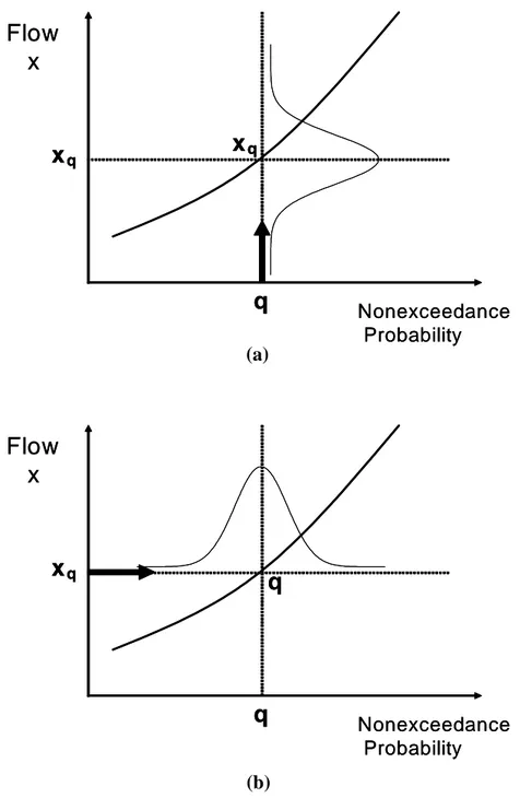
(4) Salas et al.. 4. Uncertainty of the Return Period and Risk of Failure Some investigators have recognized the uncertainty of the return period for extreme hydrologic events such as extreme rainfall and floods. Davis et al. (1972) using Bayesian approaches studied the distribution of the return period of maximum point rainfall when uncertainty arises in the parameters of the assumed Poisson and exponential distributions. Likewise, in the context of designing coastal protection works and channel improvement, Watt and Wilson (1978) presented a method in which the uncertainty associated with return period was taken into account. Also, for frequency analysis based on partial duration series, Rasmussen and Rosbjerg (1989) introduced the concept of expected risk and Rasmussen and Rosbjerg (1991) examined the precision of a design flood with exponentially distributed exceedances and Poissonian occurrence times for both seasonal and non-seasonal partial duration series. In designing flood related hydraulic structures, it is a common practice to specify a return period and derive the corresponding design size (design flood) of the structure from the frequency distribution of the annual floods. Thus, traditionally, the return period T = 1 /(1 − q ) is specified and the design flood xq obtained from the selected cumulative distribution function F(x) as the solution of xq in the equation F ( xq ) = q . This case is illustrated graphically in Fig. 1(a). The figure also shows the associated uncertainty of the design flood x q for a fixed return period or non-exceedance probability q. Another case that arises in actual practice relates to projects that have been operating for some time. After the construction of a given hydraulic structure and after some years in which the project has been operating, it may be desirable to re-evaluate the capacity of the structure. This may be desirable because of several reasons, e.g. the occurrence of extreme floods after the construction of the structure, the collection of several more years of flood data, the development of more accurate methods of analysis or the modification of design manuals and procedures, and perhaps changes in the hydrologic regime as a result of climate variability or changes in the landscape and land use, etc. In any case, re-evaluating the capacity of the structure (e.g. the capacity of a spillway) means that the flood magnitude (of the structure) is known and one may like to re-calculate certain performance statistics such as the return period (or exceedance probability) and risk of failure (or reliability). This second situation is illustrated in Fig. 1(b) where the design flood magnitude xq is known and the problem is estimating the non-exceedance probability q. In this case, q is the uncertain quantity (and consequently p, T, and R) as shown in Fig. 1(b). In this section of the paper, a method that accounts for the uncertainty in estimates of the risk of failure R is described. The method expands on the work previously reported by Salas and Heo (1997). For this purpose, the Gumbel distribution is assumed as the underlying probability model of annual flood peaks and the estimation methods based on moments (MOM), probability weighted moments (PWM), and maximum likelihood (ML) are utilized..  Hydrology Days 2003. 156.

(5) The Axis of Risk and Uncertainty in Hydrologic Design. Flow x. xq. xq. q. Nonexceedance Probability. (a). Flow x. xq. q. q. Nonexceedance Probability. (b) Figure 1. Schematic showing the uncertainty of (a) the flood quantile and (b) the non-exceedance probability. The cumulative distribution function of the Gumbel model is given by.   x − x0   F ( x) = exp− exp −  α    .  Hydrology Days 2003. 157. (2).

(6) Salas et al.. in which x0 and α are the location and the scale parameters, respectively. The parameters may be estimated from the sample X 1 ,..., X N where N is the sample size. Let xˆ 0 and αˆ denote the estimators of x0 and α , respectively. Thus, for a given design flood peak x q , one can get the corresponding nonexceedance probability q from Eq.(2). Since q depends on the unknown parameters x0 and α , the estimator of q is given by   x q − xˆ 0   qˆ = exp− exp −  αˆ    . (3). Likewise, from Eq.(1) the estimator of the corresponding risk of failure Rˆ in an n-year period is given by Rˆ = 1 − (1 − pˆ ) n = 1 − qˆ n. (4). Our concern is in assessing the uncertainty of this estimator of risk of failure. From Eq.(4) the first order approximation of the expected value of Rˆ is given by n E ( Rˆ ) ≈ 1 − [E (qˆ )]. (5). Also from Eq.(3) the term E (qˆ ) in (5) may be approximated by   x q − E ( xˆ 0 )   E (qˆ ) ≈ exp− exp −  E (αˆ )    . (6). If xˆ 0 and αˆ are unbiased, or nearly so, then E (qˆ ) ≈ q and consequently Eq.(5) may be written as    x q − x0 E ( Rˆ ) ≈ 1 − q = 1 − exp− exp − α    n.   . n. (7). ˆ can be deLikewise, the first order approximation of the variance of R rived as 2. 2.  ∂Rˆ   ∂Rˆ   ∂Rˆ   ∂Rˆ   Var ( xˆ0 ) + 2     Cov( xˆ0 ,αˆ ) +   Var ( Rˆ ) ≈    ∂xˆ   ∂αˆ   ∂αˆ  Var (αˆ ) (8)  ∂xˆ0  µ  0 µ  µ  µ where ( )µ implies that the random variables in the derivatives are replaced by their corresponding expected values. The derivatives in Eq.(8) may be obtained from (4) as. [. ]. n ∂Rˆ n = exp − yˆ − ne − yˆ = (− ln qˆ ) qˆ n αˆ ∂xˆ 0 αˆ. and  Hydrology Days 2003. 158. (9).

(7) The Axis of Risk and Uncertainty in Hydrologic Design. ∂Rˆ n = − (− ln qˆ )ln (− ln qˆ ) qˆ n ∂αˆ αˆ. (10). where yˆ = ( x − xˆ0 ) / αˆ = − ln[− ln qˆ ] is the Gumbel reduced variate. The variances and covariance in Eq.(8) and the derivatives in (9) and (10) depend on the estimation procedure. Table 1 gives the variances and covariances of the parameters estimators based on the methods of moments (MOM), probability weighted moments (PWM), and maximum likelihood (ML). Then, after appropriate substitutions and simplifications the variances of Rˆ are obtained for the three estimation methods as shown respectively in Eqs. (11), (12), and (13).. [. ] [. n2 Var ( Rˆ ) MOM ≈ exp − 2 y − 2ne − y × 1.168 + 0.192 y + 1.10 y 2 N Var ( Rˆ ) PWM ≈. [. n2 exp − 2 y − 2ne − y N ( N − 1). ]. (11). ]. × [1.128 N − 0.9066 − (0.4574 N − 1.1722) y + (0.8046 N − 0.1855) y 2 ] (12). [. ][. n2 Var ( Rˆ ) ML ≈ exp − 2 y − 2ne − y × 1.1086 + 0.5140 y + 0.6079 y 2 N. ]. (13). where y = − ln[− ln q ].. Table 1. Variances and covariances of parameter estimators for the MOM, PWM, and ML estimation methods Estimation method. Variances and Covariances MOM Var ( xˆ0 ) Var (αˆ ). Cov( xˆ0 ,αˆ ) References. 1.168 1.10. α2 N. α2. 0.096. N ( N − 1) N ( N − 1). 2. N NERC, 1975.  Hydrology Days 2003. α2 α2. N. α. PWM. −. α. ML. (1.128N − 0.9066). 1.1086. (0.8046 N − 0.1855). 0.6079. 2. (0.2287 N − 0.5861) N ( N − 1) Phien, 1987. 159. 0.2570. α2 N. α2 N. α2. N NERC, 1975.

(8) Salas et al.. 5. Comparison of Estimates The variances of the estimators of the risk of failure Rˆ based on the MOM, PWM, and ML methods can give significant differences depending on the particular values of the parameters involved. For the three estimation methods the variances of Rˆ are functions of the design life n, the non-exceedance probability q (or return period T), and the sample size N. The expected values and the standard deviations of Rˆ based on the three estimation methods are shown in Table 2 for sample size N = 10, 50, 100, design life n= 10, 50, and non-exceedance probability q= 0.90, 0.99. The expected values and standard deviations of Rˆ shown in Table 2 indicate the order of magnitude and significance of the uncertainty of such estimator. For example, for N=50, n=10, and q=0.99, Table 2 gives E (Rˆ ) =0.096 and σ (Rˆ ) =0.052 or about 54% of coefficient of variation. The implication of this result from a practical standpoint is that the designer of a hydraulic structure must be aware that setting a particular value of the risk of failure of a structure (for example, 10%) may not be a sound design criteria if the uncertainty of the estimate of such risk is significant. In fact, in some cases, especially for small values of N the coefficient of variation of Rˆ could become greater than 100%. In addition, simulation experiments have been conducted to assess the performances of the derived variances of risk of failure (based on the three estimation methods) for finite sample sizes. For this purpose, random samples were generated from the Gumbel distribution with a fixed location parameter x0 = 1000 and scale parameters 503, 1006, and 2012. The referred parameter set corresponds to coefficients of variation equal to 0.5, 1.0, and 2.0, respectively. Also the simulation experiments were made for the following cases: sample size N = 10, 25, 50, 100, and 200, design life n = 10, 25, 50, 100, 200, 500, and non-exceedance probability q = 0.90, 0.96, 0.98, 0.99, 0.995, and 0.998. Thus, for a given parameter set x0 and α , and fixed values of N, n, and q, 10,000 samples were generated. From each generated sample i (i=1,…, 10,000), the Gumbel model parameters xˆ0 (i ) and αˆ (i ) were estimated using a particular estimation method, then the risk of failure Rˆ (i ) , (i=1, …, 10,000) was determined from Eqs. (3) and (4). Subsequently, the sample mean m(Rˆ ) and the sample variance s 2 ( Rˆ ) of Rˆ (i ) were obtained. On the other hand, using the assumed “population” parameter set x0 and α (based on which the random sample was generated), the expected risk E (Rˆ ) and the variance of the risk Var (Rˆ ) were computed from Eqs. (7) and (11) or (12) or (13) depending on the estimation method. Finally, the relative bias RBIAS and relative root mean square error RRMSE of Rˆ were determined. Complete results are described in detail in Salas et al. (2003). Overall, the PWM gave the smallest RBIAS when sample size is small while ML gave the smallest biases for relatively large sample size regardless of design life. Also regarding.  Hydrology Days 2003. 160.

(9) The Axis of Risk and Uncertainty in Hydrologic Design. the RRMSE, PWM performs quite well for small sample size and large design life while ML does quite well for large sample sizes. Table 2. Expected value and standard deviation of the hydrologic risk as a function of n, q, and N based on the MOM, PWM, and ML estimation methods. N 10. q 0.90 0.99. 50. 0.90 0.99. 100. 0.90 0.99. Method MOM PWM ML MOM PWM ML MOM PWM ML MOM PWM ML MOM PWM ML MOM PWM ML. n=10. n=50. E ( Rˆ ). σ ( Rˆ ). E ( Rˆ ). σ ( Rˆ ). 0.651. 0.3111 0.2525 0.2686 0.1447 0.1216 0.1162 0.1391 0.1074 0.1201 0.0647 0.0520 0.0519 0.0984 0.0755 0.0849 0.0457 0.0366 0.0367. 0.995. 0.0230 0.0187 0.0198 0.4839 0.4067 0.3886 0.0103 0.0079 0.0089 0.2164 0.1741 0.1739 0.0073 0.0056 0.0063 0.1530 0.1224 0.1229. 0.096 0.651 0.096 0.651 0.096. 0.395 0.995 0.395 0.995 0.395. 6. Application The proposed uncertainty analysis is illustrated using the case of the Aare River at Bern-Schönau in Switzerland. The analysis is concerned with the periodical re-evaluation of the flood conveyance capacity of river reaches flowing through areas characterized by high damage potential. The Aare River drains a catchment bounded by the Swiss Central Alps, with altitudes varying up to 4000 masl, and drains snow-dominated and glacier areas. Also, the basin has a large number of artificial lakes and some regulated natural lakes. The area downstream from Bern is also characterized by some large natural lakes. As early as in the nineteenth century major hydraulic works were constructed aimed at improving the regulation of the lakes for water conservation and flood control. Between the 1960s and the 1970s new regulation criteria were developed and implemented and additional water projects constructed. The conveyance capacity of the river cross section at Bern-Schönau is 500 3 m /s, which was judged to be adequate at the time. Flood frequency analysis based on the annual maximum flood records for the period 1918-1962 (or N=45 years) using the Gumbel distribution and the method of moments sug-.  Hydrology Days 2003. 161.

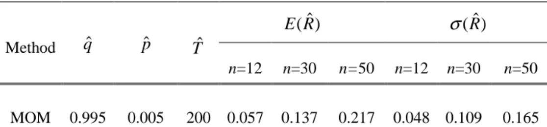
(10) Salas et al.. gested that the referred conveyance capacity corresponds approximately to a 200 years return period event, i.e. T=200. Under the assumption that the regulation plans of the complex river system would remain in place during a 30-year time span, the procedure presented in this paper enables one estimating the uncertainty associated with the hydrologic risk over the 30 years time frame i.e. (n=30). This would provide, in addition to the expected value of the risk, a further quantitative measure that may help in assessing the need of increasing the conveyance capacity of the referred river system. The dual problem can be also analyzed. Given an accepted level of an allowable risk considering its uncertainty, one may estimate the range of design life (in this case, perhaps more properly called planning horizon), which is consistent with such a risk. This may useful for planning new re-evaluations, further technical improvement and expansions as the case may be. Both cases are illustrated in Table 3. It can be observed that the uncertainty of the hydrologic risk for an expected planning horizon of 30 years is significantly large, and should not be ignored. Indeed, the expected risk E (Rˆ ) for the 200 years return period event is about 0.14 and the corresponding standard deviation σ (Rˆ ) is about 0.11 based on the MOM estimation method. Thus considering one standard deviation up, the risk could be of the order of 0.25. This means that over the given 30-year period, floods greater than the 200-year flood may occur event can occur 25% of the time. Furthermore, assuming that 10% is an acceptable risk, and considering the uncertainty of the risk as noted above, the Table 3 also suggests that such a risk level will be achieved for a planning horizon of about 12 years.. Table 3. Expected values and standard deviations of the risk based on the MOM method for the Aare River at Bern-Schönau, Switzerland.. σ (Rˆ ). E (Rˆ ) Method. MOM. qˆ. 0.995. pˆ. 0.005. Tˆ. 200. n=12. n=30. n=50. n=12. n=30. n=50. 0.057. 0.137. 0.217. 0.048 0.109. 0.165. Acknowledgment. The supports of the NSF Grant CMS-9625685 on "Risk and Uncertainty Analysis under Extreme Hydrologic Events" and the Internal Research Fund of Yonsei University are gratefully acknowledged. The Swiss Federal Office for Water and Geology provided the annual flood records of the Aare at Bern-Schönau..  Hydrology Days 2003. 162.

(11) The Axis of Risk and Uncertainty in Hydrologic Design. References Benjamin, J.R. and C.A. Cornell, 1970: Probability, statistics and decision for civil engineers. McGraw Hill Book Co., N.Y. Chow, V.T., D.R. Maidment, and L.W. Mays, 1988: Applied hydrology. McGraw Hill Book, Co., N.Y. Chowdhury, J.U. and J.R. Stedinger, 1991: Confidence intervals for design floods with estimated skew coefficient. ASCE J. Hydr. Engrg., 117(HY1), 811-831. Davis, D., L. Duckstein, C. Kisiel, and M. Fogel, 1972: Uncertainty in the return period of maximum events: A Bayesian approach. Proc. Inter. Symp. on Uncertainties in Hydrologic and Water Resources Systems, Tucson, Arizona, 853-862. DeMichele, C. and R. Rosso, 2001: Uncertainty assessment of regionalized flood frequency estimates. ASCE Journal of Hydrologic Engineering, 6(6), 453-459. Kite, G.W. 1988: Frequency and risk analysis in water resources. Water Resources Publications, Littleton, Colorado. Lee, H.L. and L.W. Mays, 1986. Hydraulic uncertainties in flood levee capacity. ASCE J. Hydr. Engrg., 112(10), 928-934. Loaiciga, H.A. and M.A. Mariño, 1991: Recurrences interval of geophysical events. ASCE. J. Water Resour. Plann. and Mgmt., 117(3), 367-382. NERC (National Environment Research Council), 1975: Flood studies report. Vol. 1, hydrological studies, Whiterfriars Press Ltd., London. Phien, H.N., 1987: A review of methods for parameter estimation for the extreme value type-1 distribution. J. Hydrol., 90, 251-268. Plate, E.J. and Ihringer, J., 1986: Failure probability of flood levees on a tidal river. Stochastic and risk analysis in hydraulic engineering, B.C. Yen, ed., Water Resources Publications, Littleton, Colorado. Rao, A.R. and K.H. Hamed, 2000: Flood Frequency Analysis. CRC Press, London. Rasmussen, P.F. and D. Rosbjerg, 1989. Risk estimation in partial duration series. Water Resour. Res., 25(11), 2319-2330. Rasmussen, P.F. and D. Rosbjerg, 1991. Prediction uncertainty in seasonal partial duration series. Water Resour. Res., 27(11), 2875-2883. Rosbjerg, D. and H. Madsen, 1992: Prediction in partial duration series with generalized Pareto-distributed exceedances. Water Resour. Res., 28(11), 3001-3010. Salas, J.D. and J.H. Heo, 1997: On the uncertainty of risk of failure of hydraulic structure. Managing water: coping with scarcity and abundance, IAHR Congress, San Francisco, 506-511. Stedinger, J.R., R.M. Vogel, and E. Foufoula-Georgiou, 1993: Frequency analysis of extreme events. Handbook of hydrology, D.R. Maidment, ed., McGraw Hill Book Co., New York. Tung, Y.K. and L.W. Mays, 1981: Risk models for levee design. Water Resour. Res., 17(4), 833-841. USIAC (U.S. Interagency Advisory Committee on Water Data), 1981: Guidelines for determining flood flow frequency. Bulletin 17B, Office of Water Dta Coordination, U.S. Geological Survey, Reston, VA.  Hydrology Days 2003. 163.

(12) Salas et al.. Viessman, W. and G.L. Lewis, 1996: Introduction to hydrology. 4th Ed., Harper Collins College Pub., New York. Vogel, R.M., 1987: Reliability indices for water supply systems. ASCE J. Water Resour. Plann. and Mgmt., 113(4), 563-579. Watt, W.E. and K.C. Wilson, 1978: An approach to optimal design of hydraulic structures. Reliability in water resources management, E.A. McBean et al., eds., Water Resources Publications, Littleton, Colorado, 75-90. Yen, B.C., 1970: Risks in hydrologic design of engineering projects. ASCE J. Hydr. Engrg., 96(HY4), 959-966. Yen, B.C. and A.H.S. Ang, 1971: Risk analysis in design of hydraulic projects. Stochastic hydraulics, C.L. Chiu, Ed., Proc. First Inter. Symp., University of Pittsburgh, Pittsburgh, Pennsylvania, 694-701. Yen, B.C., S.T. Cheng and C.S. Melching, 1986: First order reliability analysis. Stochastic and risk analysis in hydraulic engineering, Water Resources Publications, Littleton, Colorado, 1-36. Yen, B.C. and Y.K. Tung, 1994: Reliability and uncertainty analyses in hydraulic design. American Society of Civil Engineers, New York, 291p..  Hydrology Days 2003. 164.

(13)

No results found