DISSERTATION
AEROSOL IMPACTS ON DEEP CONVECTIVE STORMS IN THE TROPICS: A COMBINATION OF MODELING AND OBSERVATIONS
Submitted by Rachel Lynn Storer
Department of Atmospheric Science
In partial fulfillment of the requirements For the Degree of Doctor of Philosophy
Colorado State University Fort Collins, Colorado
Fall 2012
Doctoral Committee:
Advisor: Susan C. van den Heever Graeme L. Stephens
Richard H. Johnson Richard Eykholt
ABSTRACT
AEROSOL IMPACTS ON DEEP CONVECTIVE STORMS IN THE TROPICS: A COMBINATION OF MODELING AND OBSERVATIONS
It is widely accepted that increasing the number of aerosols available to act as cloud condensation nuclei (CCN) will have significant effects on cloud properties, both microphys-ical and dynammicrophys-ical. This work focuses on the impacts of aerosols on deep convective clouds (DCCs), which experience more complicated responses than warm clouds due to their strong dynamical forcing and the presence of ice processes. Several previous studies have seen that DCCs may be invigorated by increasing aerosols, though this is not the case in all scenarios. The precipitation response to increased aerosol concentrations is also mixed. Often precip-itation is thought to decrease due to a less efficient warm rain process in polluted clouds, yet convective invigoration would lead to an overall increase in surface precipitation. In this work, modeling and observations are both used in order to enhance our understanding regarding the effects of aerosols on DCCs. Specifically, the area investigated is the tropical East Atlantic, where dust from the coast of Africa frequently is available to interact with convective storms over the ocean.
The first study investigates the effects of aerosols on tropical DCCs through the use of numerical modeling. A series of large-scale, two-dimensional cloud-resolving model simula-tions was completed, differing only in the concentration of aerosols available to act as CCN. Polluted simulations contained more deep convective clouds, wider storms, higher cloud tops and more convective precipitation across the entire domain. Differences in the warm cloud microphysical processes were largely consistent with aerosol indirect theory, and the average precipitation produced in each DCC column decreased with increasing aerosol concentra-tion. A detailed microphysical budget analysis showed that the reduction in collision and coalescence largely dominated the trend in surface precipitation; however the production of rain through the melting of ice, though it also decreased, became more important as the aerosol concentration increased. The DCCs in polluted simulations contained more frequent,
stronger updrafts and downdrafts, but the average updraft speed decreased with increasing aerosols in DCCs above 6 km. An examination of the buoyancy term of the vertical velocity equation demonstrates that the drag associated with condensate loading is an important factor in determining the average updraft strength. The largest contributions to latent heat-ing in DCCs were cloud nucleation and vapor deposition onto water and ice, but changes in latent heating were, on average, an order of magnitude smaller than those in the condensate loading term. It is suggested that the average updraft is largely influenced by condensate loading in the more extensive stratiform regions of the polluted storms, while invigoration in the convective core leads to stronger updrafts and higher cloud tops.
The goal of the second study was to examine observational data for evidence that would support the findings of the modeling work. In order to do this, four years of CloudSat data were analyzed over a region of the East Atlantic, chosen for the similarity (in meteorology and the presence of aerosols) to the modeling study. The satellite data were combined with information about aerosols taken from the output of a global transport model, and only those profiles fitting the definition of deep convective clouds were analyzed. Overall, the cloud center of gravity, cloud top, rain top, and ice water path were all found to increase with increased aerosol loading. These findings are in agreement with what was found in the modeling work, and are suggestive of convective invigoration with increased aerosols. In order to separate environmental effects from that due to aerosols, the data were sorted by environmental convective available potential energy (CAPE) and lower tropospheric static stability (LTSS). The aerosol effects were found to be largely independent of the environment. A simple statistical test suggests that the difference between the cleanest and most polluted clouds sampled are significant, lending credence to the hypothesis of convective invigoration. This is the first time evidence of deep convective invigoration has been demonstrated within a large region and over a long time period, and it is quite promising that there are many similarities between the modeling and observational results.
ACKNOWLEDGEMENTS
I would like to first thank my advisor, Dr. Sue van den Heever, for all of her support, encouragement, and advice over the years. I am proud to be her first student, and I know many great scientists will follow me. I would like to extend thanks to my committee members as well. Drs. Graeme Stephens, Richard Johnson, and Richard Eykholt have offered valuable insight and my work has been better for their input.
I need to thank several people without whom this research would not have been com-pleted. Steve Saleeby, thank you for the budgeting code, and for countless modeling questions answered. Tristan L’Ecuyer, thank you for your help and insight into observational data, and for your helpful suggestions as a co-author. Matt Lebsock, thank you for providing model data, and for helpful conversations about dealing with satellite data. Natalie Tourville, thank you for keeping my computers working over the past few years. All of the members of the van den Heever research group have been a great help, and I think them all for the useful conversations and the fun ones. I need to express my gratitude to my friends and family who have supported me through this process, and haven’t let a crazy, stressed out grad student scare them away.
This work was funded by the National Science Foundation under Grant NSFATM-513 0820557.
TABLE OF CONTENTS
ABSTRACT . . . ii
ACKNOWLEDGEMENTS . . . iv
TABLE OF CONTENTS . . . v
1 General Introduction . . . 1
2 Microphysical Processes Evident in Aerosol Forcing of Tropical Deep Convection 3 2.1 Introduction . . . 3
2.2 Model description and experiment setup . . . 7
2.3 Results . . . 9
2.4 Conclusions . . . 18
3 Observations of aerosol induced convective invigoration in the tropical East Atlantic 32 3.1 Introduction . . . 32
3.2 Data and Methods . . . 34
3.3 Results . . . 36
3.4 Discussion . . . 41
4 General Conclusions . . . 52
4.1 Summary . . . 52
4.2 Conclusions and Recommendations for Future Work . . . 55
LIST OF TABLES
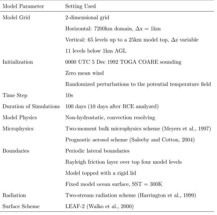
1 Model setup and parameterizations used in the simulations. . . 31 2 Difference between “Polluted” and “Clean” DCCs for each sample. Values
LIST OF FIGURES
1 Statistics over the whole model domain, for ten days after RCE was reached: (a) total number of deep convective profiles analyzed for each model run; (b) the average width of deep convective storms for each simulation; (c) convective precipitation, as a percent of total domain-wide precipitation; and (d) counts of cloud top heights for each simulation, plotted as a percent of the total domain. The cloud tops are split into low clouds (cloud top below the freezing level (about 4.4 km)), medium clouds (those with a cloud top between 4.4 and 10 km), and high clouds (cloud top above 10 km). . . 22 2 Mean number concentration (left) and the averaged mass-weighted mean
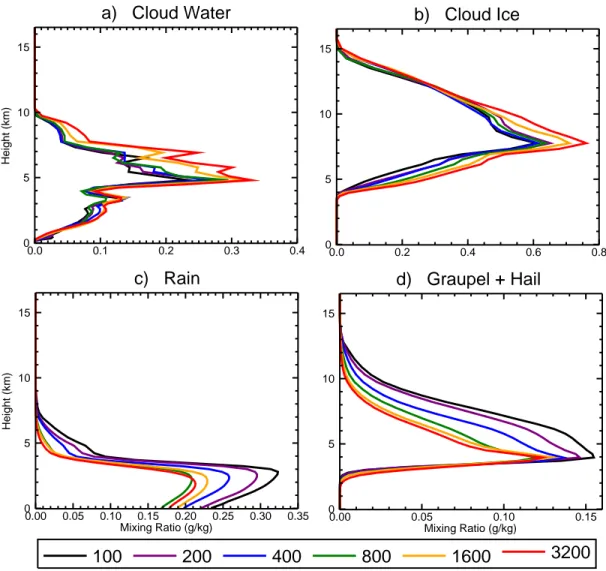
di-ameter (right) of (a,b) cloud drops, (c,d) rain drops, and (e,f) hail, averaged over DCC profiles. . . 23 3 Average profiles of mixing ratio for (a) cloud water, (b) cloud ice (pristine
ice, snow and aggregates), (c) rain, and (d) graupel and hail in DCC profiles. Units are g/kg. . . 24 4 (a) Mean surface precipitation, averaged over DCC profiles. Precipitation
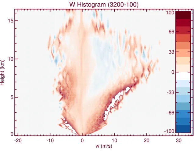
is plotted as a percent of the clean (100 cm−3) run. (b) Average profile of processes important to the production of rain in DCCs, for the clean run. (c) Mean vertically integrated values of rain production terms in DCCs. Note, the “vap to rain” term is small relative to the other terms, and is left out of this plot. (d) Average mass of hail melted in DCCs, as a difference from the clean run. . . 25 5 Histogram of vertical velocity, displayed as a difference (in percent of sample
in DCCs) between the 3200 cm−3 run and the clean run. . . 26 6 Average updraft (w > 1m/s) in DCCs, plotted as a difference from the clean
run. . . 27 7 a) The increase in temperature due to latent heating (Term 1 in Eqn. 1).
b) Loss of buoyancy due to condensate loading (Term 2 in Eqn. 1). c) The buoyancy term plotted as a difference from the clean run. The differences between model runs in this term are an order of magnitude larger than in Term 1. d) The total buoyancy as calculated in Eqn. 1, plotted as a difference from the clean run. Terms are average profiles in DCCs. . . 28 8 Average profiles of the processes that contribute to latent heating in DCCs for
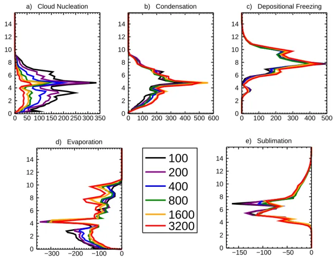
(a) the clean (100 cm−3) run and (b) the most polluted (3200 cm−3) run. . . 29 9 Average profiles of (a) cloud nucleation, (b) condensation, (c) depositional
freezing, (d) evaporation, and (e) sublimation, the most important processes involved in latent heat release in DCCs. Units are mixing ratio (g/kg). . . 30 10 The region analyzed in this study is shown here. In the inset, the frequency
of occurrence of deep convective clouds is contoured. . . 43 11 A contoured frequency by altitude diagram (CFAD), showing the frequency of
occurrence of values of reflectivity at different heights for the total sample of deep convective clouds sampled in this study. . . 44
12 A histogram showing the frequency of occurrence of values of aerosol optical depth. Vertical dashed lines denote the divisions between the ten aerosol bins used to split up the data. . . 45 13 Average values of a) center of gravity, b) cloud top, c) rain top, and d) ice
water path for each aerosol bin. . . 46 14 Histograms showing the frequency of occurrence of a) convective available
potential energy (CAPE) and b) lower tropospheric static stability. Vertical dashed lines denote the divisions between high, medium, and low values for each environmental parameter. . . 47 15 Average values of a) center of gravity, b) cloud top, c) rain top, and d) ice
water path for each aerosol bin. Deep convective clouds are split by high, medium, and low CAPE. . . 48 16 As in Figure 6, but profiles are split up by LTSS. . . 49 17 a) A difference CFAD, calculated by subtracting normalized CFADs from the
most polluted and cleanest aerosol bins. b) A two-dimensional histogram showing the difference in the frequency of occurrence of values of cloud top and rain top between the polluted and clean samples. . . 50
1 GENERAL INTRODUCTION
It has been known for many years that aerosols can impact important microphysical and dynamical properties of clouds (Twomey, 1977; Albrecht, 1989); however, these effects are complicated and may depend on cloud type (Seifert and Beheng, 2006; van den Heever et al., 2011) and environment (Khain et al., 2008; Lebsock et al., 2008; Fan et al., 2009; Storer et al., 2010). It has proven particularly difficult to understand the changes that occur in deep convective clouds (DCCs) for two main reasons: (1) the presence of ice in these clouds adds additional uncertainty to processes such as precipitation formation, and (2) DCCs can form in many types of environments in association with differing types of forcing. Much of the research performed that has examined aerosol indirect effects on DCCs, as summarized by Khain (2009) and Tao et al. (2012), has had mixed results both in terms of the effect of aerosols on the precipitation produced by these clouds, as well as whether convective invigoration occurs in polluted storms. The purpose of the work summarized here is therefore to add to the knowledge of how the presence of increased aerosols can impact DCCs, through a combination of modeling and observational analysis.
This dissertation is split into two main components. Chapter 2 describes a modeling study undertaken in order to learn the important processes occurring in DCCs that are affected by increasing aerosol concentrations. A series of large scale, two-dimensional model runs were completed, with only the aerosol concentration differing, and a large sample of DCCs was analyzed for aerosol effects. The microphysical budget was examined in detail in order to distinguish which processes were important for precipitation formation and latent heating, and to examine how these processes were affected by the presence of increased numbers of aerosols. This chapter has been submitted, in this form, as a manuscript to the Journal of Atmospheric Science, and has been accepted pending revisions.
Up until now, no observational studies have been published in which aerosol impacts on deep convection are examined over a large spatial and temporal scale. Other observational studies on aerosol indirect effects have focused on a very limited spatial domain, or did not isolate the impacts specifically on deep convection. In order to evaluate whether the aerosol indirect effects described in the modeling study can be observed, a study was performed utilizing CloudSat data; this research is summarized in Chapter 3. Four years of satellite data were analyzed in a region of the East Atlantic in keeping with the conditions simulated in Chapter 2. A large sample of DCCs was acquired over a four year period and matched with aerosol optical depth (AOD) information obtained from a global transport model. Four parameters (center of gravity, cloud top, rain top, and ice water path) were examined for differences associated with changes in AOD. An attempt was made to separate out environmental effects from the effects of aerosols by splitting the data up by convective available potential energy (CAPE) and lower tropospheric static stability (LTSS), and the results were tested for significance. This chapter is a manuscript in preparation to be submitted to a peer-reviewed journal.
2 MICROPHYSICAL PROCESSES EVIDENT IN AEROSOL FORCING OF TROPICAL DEEP CONVECTION
2.1 INTRODUCTION
Tropical convection is a key component of the climate system, playing an important role in linking radiation, dynamics, and the hydrologic cycle in the atmosphere (Arakawa, 2004). Deep tropical convection in particular is a significant source of precipitation (Haynes and Stephens, 2007; Liu, 2011), and acts to transport heat upwards through the troposphere with vertical motions and the release of latent heat. In addition, the deep convective clouds that form in the tropics are necessary for the global circulation of the atmosphere, as they are the primary means by which energy is transported from the tropics to the midlatitudes (Riehl and Malkus, 1958; Fierro et al., 2009, 2012).
The importance of convection to the climate system dictates that an effort be made to understand factors, environmental and otherwise, that can influence tropical convective clouds. The focus of this study is on aerosol indirect effects, a key uncertainty in our cur-rent and changing climate (Solomon et al., 2007). Particularly, the goal is to understand changes that can occur, to precipitation amount and storm strength, in tropical deep con-vective clouds due to an increase in the environmental concentration of aerosols (both nat-ural and anthropogenic) that can act as cloud condensation nuclei. This study investigates these aerosol indirect effects on tropical deep convection utilizing a series of large-scale, high-resolution simulations run under a radiative-convective equilibrium framework. The simulations were performed using a cloud resolving model with detailed microphysics, and the budgets of various hydrometeors and microphysical processes were examined in order to point to the key changes impacting deep convection.
2.1.1 Tropical convection and radiative-convective equilibrium
It has been observed that tropical convection is typically organized in a trimodal distribution (Johnson et al., 1999; Posselt et al., 2008), with the three peaks corresponding to shallow trade-wind cumulus, cumulus congestus, and cumulonimbus clouds. This study is concerned with the deep convective clouds (DCCs) that typically extend through the depth of the tro-posphere. In the tropics, DCCs are a ubiquitous feature that often organize into larger-scale structures such as squall lines (Rickenbach and Rutledge, 1998). DCCs are also responsible for a significant portion of the rainfall in the tropics, particularly in the Intertropical Con-vergence Zone (ITCZ) and the west Pacific warm pool region (Haynes and Stephens, 2007). Liu (2011) showed that in many regions in the tropics, over 50% of the rainfall could be attributed to raining precipitation features with radar echo top heights above 10km.
In this study, tropical DCCs will be examined within the framework of radiative-convective equilibrium (RCE). A simple radiative equilibrium assumption leaves the atmo-sphere absolutely unstable to vertical motions. By allowing convection, latent and sensible heat can be transported vertically and released in the upper troposphere, removing this in-stability. Over a sufficiently long temporal integration, the modeled atmosphere will relax to an equilibrium state, with a cooler surface and warmer upper troposphere than the initial state. The vertical profiles of the atmosphere created in RCE simulations are quite similar to those that have been observed in the tropical atmosphere. Several studies (Held et al., 1993; Tompkins and Craig, 1998; Bretherton et al., 2005; Stephens and van den Heever, 2008; van den Heever et al., 2011) have successfully used the RCE framework to simulate the climate state of the tropics.
2.1.2 Aerosol indirect effects
The first and second aerosol indirect effects (Twomey, 1977; Albrecht, 1989) together explain the behavior of warm clouds in polluted environments, that is environments with more aerosols available to act as cloud condensation nuclei (CCN). In situations of equal liquid
water content, polluted clouds will have more and smaller cloud droplets, higher albedos, and will produce less warm rain due to a less efficient collision/coalescence process. While there can be some differences in these effects (both in magnitude and sign) due to cloud type (Seifert and Beheng, 2006; van den Heever et al., 2011) and environment (Khain et al., 2008; Lebsock et al., 2008; Fan et al., 2009; Storer et al., 2010), many aspects of aerosol indirect effects on warm clouds are fairly well understood.
The addition of ice, however, leads to a much more complex response. In particular, the response of deep convective clouds to aerosol forcing is currently not well understood. Throughout the warm cloud depth, these clouds appear to behave similarly to simple cumu-lus clouds or a stratocumucumu-lus deck - they have more, smaller cloud droplets and less efficient warm rain production (van den Heever et al., 2006; Rosenfeld et al., 2008; Storer et al., 2010; Tao et al., 2012). The consensus in previous work seems to indicate that deep convective clouds formed in polluted environments will contain larger amounts of cloud water due to the suppressed warm rain process. It follows then that more ice will form as this additional cloud water is lofted above the freezing level. The increased ice amounts can then influ-ence other important aspects of the storm. The formation of the increased ice amounts is postulated to lead to a larger latent heat release, which can enhance storm updrafts thus producing convective invigoration (Andreae et al., 2004; Khain et al., 2005; van den Heever et al., 2006). Convective invigoration is likely to result in increased surface precipitation to-tals. Additionally, the presence of increased ice mass in polluted storms may lead to changes in the production of precipitation through melting processes. The combination of convective invigoration and the additional pathways for precipitation formation may lead to a precip-itation gain that can counteract, or even overcome, the loss in warm rain, leading to a net increase in accumulated precipitation.
Several modeling (Khain et al., 2005; van den Heever et al., 2006; van den Heever and Cotton, 2007; Lee et al., 2008a) and observational (Andreae et al., 2004; Rosenfeld et al., 2008) studies have found evidence of convective invigoration. However Storer et al.
(2010) did not see any evidence of supercell storm strength being impacted by aerosols, and the question of invigoration or suppression of convection may strongly depend on the environment (Khain et al., 2008; Fan et al., 2009). Concerning precipitation produced by deep convective storms in polluted environments, the results were again mixed. Khain (2009) made an attempt to classify the effects of aerosols on deep convective precipitation by analyzing a number of previous studies in terms of a mass budget. The general trend found was that in polluted storms, there was an increase both in condensation and in condensate loss through the increase in evaporation with smaller cloud drops. This study proposed that the net effect on precipitation could be found to depend on the difference in the changes of those two terms. Therefore, in studies of deep convection in dry environments the increase in condensate loss was greater than that of condensate gain and so precipitation was suppressed in polluted scenarios, whereas the reverse would occur in moist environments and an increase in precipitation could be found. Other recent studies have found that atmospheric stability (Storer et al., 2010) and shear (Fan et al., 2009) can also act to modulate the effects of aerosols on precipitation in convective storms.
With all of the mixed results that have been found, it remains clear that while ice plays an important role in aerosol/convection interactions, the details are not currently well under-stood. It has been suggested that convective invigoration may be brought about by increases in latent heating due to the freezing of cloud water. However, this is not the only process act-ing in deep convective clouds. Multiple processes involvact-ing phase changes (rimact-ing, meltact-ing, vapor deposition, etc.) all occur simultaneously, and it is not well known exactly how all of these processes interact to produce latent heat within convective clouds. Similar uncertainty exists surrounding the question of aerosol impacts on surface precipitation. Again, this is because there are multiple processes that act to form precipitation in deep convective clouds (such as the melting of hail and other ice species in addition to the warm rain process). It is not currently known how aerosols can affect all of these various processes, making the net effect of aerosols on surface precipitation difficult to predict.
In this study, the effects of aerosols on DCCs will be examined within a series of large-scale, two-dimensional, cloud resolving simulations set up using a radiative-convective equi-librium (RCE) framework. The RCE framework offers the ability to simulate a large-scale, idealized tropical atmosphere, including realistic cloud populations. The analysis presented will concentrate on aerosol effects on deep convective clouds, of which there are a large sample in each simulation. A detailed examination of the microphysics budget will be undertaken in order to understand the processes important to convective invigoration and surface pre-cipitation, and how these processes are affected by an increase in aerosols that can act as CCN.
2.2 MODEL DESCRIPTION AND EXPERIMENT SETUP
The Regional Atmospheric Modeling System (RAMS) (Pielke et al., 1992; Cotton et al., 2003) version 6.0 was used for the simulations described here. RAMS is a limited area, nonhydrostatic, cloud resolving model that utilizes a detailed 2-moment microphysics scheme (Meyers et al., 1997). This microphysics scheme is considered bin-emulating, as it has the reduced computational time of a bulk scheme, while using detailed lookup tables in order to capture aspects of a bin microphysics scheme. Lookup tables are previously generated offline for several important processes such as the activation of CCN (Saleeby and Cotton, 2004), cloud drop collection (Feingold et al., 1988), and drop sedimentation (Feingold et al., 1998), through the use of a detailed parcel model. One important feature of the microphysics scheme in RAMS is the fact that CCN concentration is predicted based on background aerosol concentrations and environmental conditions, rather than prescribed (Saleeby and Cotton, 2004). Aerosols can be introduced into the model at any time step, are advected throughout the model domain, and are lost through activation. A summary of model options utilized is included in Table 1.
The simulations performed for this study are similar to those described by van den Heever et al. (2011). The model was run using a two dimensional domain in order to cover
a large zonal extent (7200 km) with sufficiently fine model resolution. By utilizing such a domain, it is possible to look at a large sample of convective clouds forming in different conditions within the same RCE model run. The model was run with a horizontal grid spac-ing of 1km, so that convection was explicitly resolved. There were 65 levels in the vertical, with stretched spacing. The model was initialized with a sounding from the Tropical Ocean Global Atmosphere Coupled Ocean Atmosphere Response Experiment (TOGA COARE) and zero mean wind. Random potential temperature perturbations were initially introduced into the boundary layer in order to initiate convection. The simulation was run out until RCE was reached (60 days). At this point, the model was restarted with the introduction of various concentrations of aerosols that can serve as CCN. The aerosol was added in a layer between 2-4 km, which is similar to the height of the Saharan dust events often seen in the tropical Atlantic (Carlson and Prospero, 1972; Karyampudi et al., 1999). While African dust is typically considered for its role as ice nuclei (Demott, 2003), recent studies (Twohy et al., 2009) have shown that dust also can be effective as CCN or giant CCN (GCCN). In this study, the aerosols are only considered for their role as CCN, in order to simplify the analysis of the interactions being investigated. Six runs were completed, identical except for the aerosol concentration in the 2-4 km layer. The aerosol concentrations were doubled from a “clean” 100 cm−3 to a very polluted 3200 cm−3. The high end of concentrations exam-ined here is out of the range of what has ordinarily been measured for Saharan dust events. For example, Zipser et al. (2009) measured particle concentrations of 300-600 cm−3 in the NASA African Monsoon Multidisciplinary Analysis (NAMMA) field campaign. However, similar concentrations have been measured in urban areas (e.g. China, as described in Rose et al., 2010) and for an idealized study such as this, the goal was to examine a wide range of possible aerosol concentrations.
For the purposes of this study, a deep convective cloud (DCC) was defined as a model column that contained cloud (total condensate > 0.01 g/kg) through a consecutive layer at least 8 km deep. The clouds studied include both single isolated deep convective towers and larger, organized cloud systems (though only in two dimensions). Additionally, the
DCC profiles analyzed include all stages in the lifetime of a deep convective storm, both new growing convection and older, more stratiform-like features that meet the depth requirement. As the domain-wide changes in microphysical processes, and not the larger scale storm organization, are the focus here, no attempt is made to separate aerosol effects based on storm type or stage of development. Unless otherwise noted, all of the fields analyzed here are averaged only over those model columns containing DCCs.
2.3 RESULTS
2.3.1 Convective organization
Before narrowing down the analysis to DCC profiles only, it is useful to examine domain-wide differences in organization brought about by changes in aerosol concentrations. Fig. 1a shows the total number of profiles that qualified as DCCs for each simulation. As stated above, a DCC is defined as a column containing cloud (total condensate > 0.01 g/kg) through a continuous depth of at least 8 km. It is clear that generally more convective profiles are present with increasing aerosol concentrations. A convective storm was defined as a series of horizontally consecutive DCCs, and the average width of these storms was calculated by simply counting DCC profiles that occurred continuously across the horizontal domain. Fig. 1b demonstrates that the average width of the deep convective storms is greater in polluted simulations; the total number of individual storms is also higher (not shown). Polluted simulations thus contain more deep convective storms, that are larger in extent than in the cleaner scenarios, lending support to the hypothesis that aerosols invigorate convection. It will be demonstrated in Section 1.3.2 that the average precipitation produced by a DCC (calculated by averaging over all DCC columns) is lower in polluted simulations. However, the total precipitation produced by DCCs increases with increasing aerosols, since there are more storms contributing to the total amount. Precipitation produced by other clouds shows a significant reduction with increasing aerosols (not shown), likely as a consequence of the second aerosol indirect effect, so the percentage contribution of deep convective storms to
the total surface precipitation is much higher in polluted simulations (Fig. 1c), given their enhanced frequency.
The polluted simulations contain more deep convective storms that are broader and have higher cloud tops (not shown). The increase in convective mass flux in polluted scenarios must be compensated for elsewhere in the model domain. A simple example of this can be seen in Fig. 1d, showing the cloud top counts over the whole model domain. It can be seen that while there is an increase in the number of high cloud tops, there is a substantial decrease in low clouds. The increased convective mass associated with convective invigoration is compensated by increased subsidence in the drier regions of the domain (van den Heever et al., 2012), thus suppressing cloud formation in the trade wind cumulus regimes. Without a detailed examination of domain-wide statistics, it is difficult to attribute cause and effect, however, it can be said that increasing the number of aerosols available to act as CCN has definitive impacts on cloud organization and structure.
2.3.2 Microphysics changes and precipitation response
Throughout the warm cloud depth of the DCCs examined here, the microphysical changes evident with increased aerosols are similar to the aerosol indirect effects initially described for shallow clouds (Twomey, 1977; Albrecht, 1989). With more aerosols available to act as CCN, more cloud drops are formed in polluted simulations and drop sizes are smaller due to greater competition for water vapor (Fig. 2). The collision and coalescence process is therefore less efficient, due to the narrower cloud droplet spectrum, and it becomes more difficult for rain drops to form. The reduced efficiency of warm rain production leads to a decrease in the mass of rain, and an increase in cloud water (Fig. 3). As shown in Fig. 2, the rain drops that do form are larger in polluted simulations. This is a combination of multiple effects. Firstly, since autoconversion is suppressed in polluted storms, more cloud water is available for accretion once rain formation begins. Thus, the rain drops that form are able to grow faster as they fall, which can be seen by the more pronounced peak in rain drop
size at around 6 km. Below the freezing level, there is another substantial peak in rain drop diameter as the melting of hail becomes an important part of rain production. Hailstones shed comparatively large rain drops, and as hail size increases the number of drops shed will increase. Thus, in polluted simulations there are more of these large drops contributing to the average rain drop size. The mean rain drop diameter also increases slightly below cloud as smaller drops will evaporate first.This increase in rain drop size with increasing aerosols is consistent both with previous model results (Altaratz et al., 2007; Berg et al., 2008; Storer et al., 2010) and observations (May et al., 2011).
Ice has a similar response to liquid water (Fig. 3), meaning there is less mass of pre-cipitation sized ice (graupel and hail), but an increase in cloud ice in polluted storms. Due to the less efficient warm rain process and increased amount of cloud water, more water can be lofted above the freezing level to produce ice. Thus, the mass of cloud ice (pristine, snow, and aggregates) increases for increased aerosol concentration. Graupel and hail show a decrease in mass similar to that of rain. These large, precipitation sized ice particles form when an aggregate or snow flake becomes sufficiently rimed. Since there are more, smaller ice particles in polluted DCCs, there is greater competition for water, and it becomes more difficult for each particle to grow to graupel size. Once graupel or hail does form in polluted simulations, the large amounts of cloud water and ice available to be accreted can lead to rapid growth, and hence the hail has larger average diameters than in the clean scenario.
As explained above, the production of warm rain in polluted clouds is less efficient due to the larger numbers of smaller cloud drops in these clouds. Though the total convec-tive precipitation in polluted simulations increases with increased aerosol loading, Fig. 4a demonstrates that the average surface precipitation for each simulation (again, the average in DCC profiles) has the opposite trend. The trend is nearly monotonic, with one outlier in the 800 cm−3 run. This simulation is an anomaly in other trends as well, however the reasons for such differences in trends are uncertain at this time.
Decreased precipitation with increased aerosol concentration is what has been typically found in previous studies concerning shallow clouds. However, it is not just collision and coalescence which acts to produce rain in DCCs - the ice phase is also an important con-sideration. The processes that contribute to the formation of rain are plotted for the clean run in Fig. 4b. “Cloud to rain” is the collision and coalescence of cloud drops to form rain drops - the warm rain process. “Vapor to rain”, a very small contribution compared to the others, consists of vapor diffusion onto rain drops. The production of rain by ice consists of two terms, “ice to rain”, the collection of ice by falling rain, and “melt hail”, the production of rain through the melting and shedding of hailstones. The melting of graupel does not contribute to precipitation in this model, as melted graupel is moved to the hail category. Both of the terms involved in the production of rain associated with ice have large positive contributions to rain formation, but only in a very narrow layer near the freezing level. There are two sinks of rain. “Rain to ice” is the collection of rain by ice species, or the riming of rain, and “rain evap” is simply the evaporation of rain.
In order to examine the average column production of rain, each of the processes involved in producing rain was vertically integrated and averaged for the columns containing DCCs. The results are shown in Fig. 4c. The reduction in the warm rain process as a result of enhanced aerosol concentrations is quite clear, the reasons for which are described above. Because less rain is produced in polluted scenarios, there are fewer rain drops to collect ice particles as they fall, thus the “ice to rain” term also shows a significant reduction with increased aerosols. The “melt hail” term decreases only slightly with increasing aerosols. Looking in more detail at the melting of hail (Fig. 4d), it becomes clear that rather than changing the amount of hail that is melted, an increase in aerosol concentration leads to a shift in where the melting is occurring. As explained above, hail stones produced in polluted storms are able to grow larger due to the more abundant amounts of cloud water available for riming (Fig. 2). Since the hail stones are larger in polluted storms, melting is less efficient and occurs through a deeper layer. In cleaner scenarios, however, smaller hail is more easily transported to the anvil regions of the storms, and so less hail is available to melt and
produce rain. The combination of these effects means that while total hail amount decreases significantly with increased aerosol concentration, the rain produced from the melting of hail only demonstrates a small change.
Also plotted in Fig. 4c are the sinks of rain, “rain to ice” and “rain evap”, both of which also decrease with increasing aerosol concentrations. “Rain to ice”, the removal of rain through riming, becomes less efficient as there is less mass of rain available to collect in the polluted simulations. The evaporation of rain also decreases with increasing aerosol concentration, because the larger rain drops in polluted simulations are less efficient at evaporating.
A point to note from Fig. 4c is that the production of rain from ice (that is, the sum of “ice to rain” and “melt hail”) is of the same magnitude or larger than that from warm rain production. As the background aerosol concentration increases and the warm rain production decreases, the production of rain through melting becomes increasingly important. Summing all of the terms in Fig. 4c, reproduces the value for the average production of rain occurring within a DCC. The average production of rain follows the trend of surface precipitation seen in Fig. 4a, confirming that the reduction in precipitation can be explained. Though the production of rain in association with ice processes also decreases with increasing aerosol concentration, it is the decrease in warm rain production that dominates the trends seen in the average surface precipitation produced within the DCC profiles.
2.3.3 Updraft strength and convective invigoration
It has been demonstrated that changes in the aerosol concentration lead to significant differ-ences in storm microphysics and precipitation production. It follows that these differdiffer-ences may then feed back on the individual storm dynamics through changes in latent heating and thus updraft strength. Shown in Fig. 5 is a histogram displaying the frequency of occur-rence of updraft and downdraft speeds as a function of height in DCCs. The frequency is normalized and then taken as a difference from the clean run, thereby demonstrating the
change with increasing aerosol concentrations. Only one histogram is shown, but in each simulation with increasing aerosols, the same general trends can be seen. At any height, there is a shift towards more frequent occurrences of the strongest updraft and downdraft magnitudes in the more polluted scenarios, in agreement with the domain-wide convective invigoration that was discussed in Section 2.3.1. In the lower levels (below about 6 km), there is a particularly clear trend - higher aerosols lead to stronger updrafts and downdrafts. Because of the wide spread of possible updraft speeds higher in the column, the trend with increasing aerosols is more complex. There are generally more of the strongest updrafts in the polluted simulations, however this is at the expense of moderate (∼ 5 − 15 m/s) updraft speeds.
A profile of average updraft velocity (updraft defined as those points with w > 1 m/s) is plotted in Fig. 6 as a difference from the clean run. Convective invigoration with increased aerosols can be seen clearly in the lower levels of the DCCs, up to about 6 km, and then the trend reverses and updrafts are weaker for higher values of aerosol loading. This trend reversal coincides with the increase in the variation of updraft speeds described above. The changes in updraft strength due to increasing aerosol concentration are more complex than shown in Fig. 6, as looking at the average can wash out changes in the extreme values. However, the potential contributions to updraft changes will be examined in an average sense, so as to identify which processes are generally most important to convective invigoration trends evident over the whole sample of DCCs.
Previous studies that have seen convective invigoration (Andreae et al., 2004; Khain et al., 2005; van den Heever et al., 2006; Rosenfeld et al., 2008; Tao et al., 2012) have hypothesized that the increase in updraft speed was brought about by an increase in the freezing of liquid cloud water to form ice. A detailed budget of the processes included in the buoyancy term of the vertical velocity equation was undertaken here in order to examine whether this is a reasonable explanation for the trends seen in this series of simulations. The vertical velocity equation is composed of three main terms: horizontal and vertical advection,
the pressure gradient term, and buoyancy, which all may be affected by the presence of aerosols. However, because the analysis has been limited to processes occurring within a single (DCC) column, and because the particular hypothesis being examined concerns latent heating, only the buoyancy term is examined here. The buoyancy term in the vertical velocity equation is shown below.
B = g(θ
0
θ0
) − gqc. (1)
The buoyancy of a parcel, B, is affected by two terms, as shown in Eqn. 1. Term 1 describes gravity (g) acting on a change in density brought about by a difference in potential temperature. In this equation, θ0 is the mean, base state potential temperature, and θ0 is
the difference in potential temperature brought about by latent heat release. Term 2 is the drag associated with the presence of liquid water and ice, or condensate loading, where qc is
the total condensate (liquid water + ice) mixing ratio.
Term 1 in Eqn. 1, the buoyancy differences brought about by changes in potential temperature due to latent heat release, is plotted in Fig. 7a. There is a slight increase in latent heating with increased aerosols, up to about 3km. The differences between the model runs become quite complex above that, however, as there are a number of processes that contribute to this latent heat term. Fig. 8 shows an average profile of the important contributions to latent heating, for the cleanest and most polluted runs. As stated earlier, aerosol indirect theory suggests that the freezing of additional cloud water is a large contri-bution that would lead to convective invigoration (Andreae et al., 2004; Khain et al., 2005; van den Heever et al., 2006; Rosenfeld et al., 2008; Tao et al., 2012). The freezing of liquid water can be represented by two terms plotted in Fig. 8: “Ice Nuc”, the nucleation of ice particles, and “Rime”, the riming of liquid water onto existing ice particles. These two pro-cesses, represented by the yellow and pink lines in Fig. 8 respectively, are not relatively large contributions to the latent heating, regardless of the aerosol concentration. It can be seen in this example that the largest positive contributions to latent heating come from cloud
nucleation, condensation, and depositional freezing, with the largest negative contributions coming from evaporation and sublimation. To see the impact of increased aerosols, these five most important processes are plotted for each model run in Fig. 9.
In the initial stages of cloud development, polluted clouds undergo much more nucleation since there are more aerosols available to be activated as CCN. However, throughout most of the lifetime of the storms in polluted scenarios, condensation by vapor diffusion onto existing cloud drops becomes a much more dominant process. This is due to the increased surface area associated with the presence of larger numbers of smaller drops. For a simple example, consider a cubic meter of cloud containing 0.5 g of liquid water. In a clean scenario, the population of cloud drops may be 10 cm−3 and in a polluted case, 100 cm−3 (see Fig. 2). If the liquid water is divided evenly among the cloud drop population (i.e. all drops are assumed to be the same size), the clean case has a cloud drop size of 22.9 microns, and the polluted case, 10.6 microns. By summing over the entire sample, the collective surface areas of the cloud drops would be 0.0656 m2 and 0.141 m2 respectively. There is roughly twice the surface area in the hypothetical polluted case, and since vapor diffusion onto cloud drops is proportional to surface area, the condensation would increase accordingly. Because there is so much competition for water vapor once such a population of cloud drops is established, new cloud drop nucleation becomes of secondary importance, as existing cloud droplets provide less of an energy barrier to condensation. Thus, when averaged over the lifetime of the DCCs, condensation shows a substantial increase with increasing aerosol concentration, while cloud nucleation decreases (Fig. 9). Other studies have shown similar increases in condensation with increased aerosol concentration (Khain et al., 2008; Lee et al., 2008b). The other important process that contributes greatly to positive latent heating in DCCs is deposition of vapor onto ice. This increases with increasing aerosol concentrations due to the fact that there is a greater mass of cloud ice and most of the cloud ice is in the form of more numerous, smaller aggregates (not shown). Thus, the same surface area effect occurs for depositional freezing as was described for condensation.
Acting to balance the positive contributions to latent heating are evaporation and sub-limation (Fig. 9). Evaporation in cloud shows a distinct increase with increasing aerosol concentrations, due to the smaller cloud drops which evaporate more easily. However, in the lower levels, evaporation actually decreases with increasing aerosol, since in this region of the cloud and below, evaporation of rain is more dominant than evaporation of cloud water, and the rain drops are larger (Fig. 2) and thus less efficient at evaporating. Sublimation decreases with increasing aerosols, which is counter to what occurs with evaporation. In-creased evaporation in cloud leads to more instances of ice supersaturation, which enhances deposition onto ice through the Bergeron-Findeisen process - so sublimation is less likely to occur in the more polluted scenarios.
The processes contributing to buoyancy through latent heating do not, on their own, explain the trend seen in the mean updraft. In the lower levels, an increase in buoyancy can be seen largely due to decreased rain evaporation (that is, reduced evaporational cooling leads to comparatively warmer air near the surface, which will be more buoyant), but there is no clear link between the latent heating term and the decreased updraft speed above 6 km. To further explain this, it is necessary to look at the condensate loading term in Equation 1. Fig. 7b shows the condensate loading, which is simply the weight of the liquid water and ice contained within the DCCs. In polluted storms, more liquid and ice exist within cloud (Fig. 3), leading to a much larger drag on the updraft from the weight of the condensate. Though the heating and condensate terms themselves (Fig. 7a and b) are of comparable magnitude, the differences between the model runs are much larger in the condensate loading term (Fig. 7c), and as such dominate the trend in total buoyancy (Fig. 7d). The large change in condensate loading leads to a decrease in buoyancy, and hence contributes to the decreased (average) updraft speed with increased aerosols above 6 km.
It has been asserted by previous studies that convective invigoration would be brought about by additional latent heat released in the freezing of cloud water. However, this study suggests that not only is the freezing of liquid cloud drops not the most important process for
the release of latent heat, but the additional mass of condensate produced can significantly reduce the buoyancy of an updraft in these tropical DCCs studied, overshadowing any latent heating effects in the upper levels. Again, a few caveats must be pointed out. Firstly, the average profile of updraft speed does not tell the whole story (as illustrated in Fig. 5). Since the domain-wide statistics discussed in Section 2.3.1 point to convective invigoration, it is likely that the effect of aerosols on storm updraft varies through the storm life cycle. If the initial deep convective cores are invigorated by increases in cloud drop nucleation, condensation, and vapor deposition, this would explain the extreme values in Fig. 5 and the higher cloud tops. The decrease in mean updraft brought about by enhanced condensate loading is likely occurring in the later, more stratiform-like stages of storm lifetime, which persist longer due to the reduction in precipitation formation in each column. It is also important to note here that the presence of shear in the environment may lead to differences in the overall response. As seen by Nicholls et al. (1988), the presence of increased shear can lead to more effectively organized storm systems with tilted updrafts, reducing the load from condensate on the updraft. The response of DCCs in a sheared environment is work that will be done in the future. Lastly, the buoyancy term is just one term in the vertical velocity equation and other possible dynamic feedbacks such as cold pools have not been examined here. However, the conclusion can still be made that convective invigoration in this study cannot be simply attributed to the release of latent heat involved in the freezing of cloud water. Other processes, such as condensation and vapor diffusion onto ice, can be of significantly greater magnitude, and the drag associated with condensate loading must be considered as well.
2.4 CONCLUSIONS
A series of large-scale, two-dimensional, RCE model simulations has been used to successfully demonstrate that significant differences in microphysics, dynamics, and large-scale organi-zation of DCCs develop from differences in background aerosol concentration. The basic
warm cloud microphysical differences have been shown to follow the traditional predictions of aerosol indirect theory, but in order to more fully explain changes in surface precipitation amount and updraft speed in DCCs, it was necessary to involve ice phase microphysics in the analysis. The complexity involved with ice phase microphysics was investigated using a de-tailed examination of the microphysical processes involved in the production of precipitation and the generation of buoyancy involved in vertical motion.
Over the whole domain, the number of deep convective storms increased in number, and in size, with increasing aerosol concentrations. Domain-wide cloud top counts showed a shift towards more high cloud tops and fewer low cloud tops, suggesting an invigoration of the DCCs when aerosol loading was increased. Additionally, the total deep convective precipitation increased with increasing aerosols, and made up a larger percentage of the total domain-wide precipitation total. The total precipitation over all cloud types in the domain did not change substantially with aerosol concentrations, as total precipitation is largely a function of the RCE constraint imposed in the simulations. Precipitation from other cloud types not examined here, such as trade wind cumulus clouds, decreased with increasing aerosol concentration.
Though the total domain-wide deep convective precipitation increased with increasing aerosol concentration due to the increased number of DCCs present, the average precipitation produced by each DCC decreased. This was due to a combination of factors. The warm rain process in the polluted simulations was less effective because of the smaller cloud drop sizes. The production of rain through ice processes (melting of hail and collection of ice by rain) also decreased with increasing aerosols, but the warm rain reduction was the dominant term in determining the average precipitation trend in DCCs. However, as the background aerosol concentration increased, the production of rain through the melting of ice became relatively more important when compared to the warm rain process. It should be noted that some precipitation was likely produced in the stratiform anvil regions associated with the DCCs studied here, which was not included in this analysis, but would likely add even more to the
convective precipitation total in polluted simulations. In general, the results presented here suggest that ice phase microphysics is an important factor when considering aerosol effects on deep convective precipitation.
Looking in more detail at the updrafts in polluted storms, it was seen that the average updraft speed decreased with increasing aerosol concentration through much of the cloud, yet those DCCs formed in polluted simulations were more likely to have stronger updrafts and downdrafts. There are more extreme values of updraft (both high and low) in polluted storms, at the expense of moderate updrafts. Previous studies that noted convective invigo-ration with increasing aerosols attributed the change in updraft speed to increases in latent heat from the freezing of a larger mass of cloud water. To examine that theory, the buoyancy term in the vertical velocity was examined in detail. The latent heat released in the freezing of cloud water to form ice was less significant compared to that released from condensation and vapor diffusion processes (both onto liquid water and ice). In addition, the larger ice amounts produced in polluted storms served to increase the condensate loading of the up-draft, which actually reversed the trend in buoyancy above the freezing level, contributing to the decrease in average updraft speed above 6 km. It should be noted that the buoyancy term is not the only possible way that vertical velocity may have been affected by aerosol concentrations. For example, changes in near-surface evaporation will affect the strength of cold pools produced by convective storms, which can then have effects on the forcing of new convection (as seen in van den Heever and Cotton (2007); Storer et al. (2010)). However, the results of this study demonstrate the importance of considering the variety of microphysical processes that contribute to latent heating within DCCs.
The fact that the average updraft speed in DCCs decreases with increasing aerosol concentrations above the freezing level seemingly argues against the domain-wide convective invigoration also discussed here (more DCCs, wider storms, higher cloud tops, and more total convective precipitation). However, the two contradictory ideas can be considered in the following manor. In the initial stages of the lifetime of a DCC, cloud drops and ice
crystals are quickly being nucleated and this nucleation, along with vapor deposition, is adding large amounts of latent heat to the column. The increased latent heat invigorates the updraft in the convective core, leading to the more frequent occurrences of high updraft magnitudes and allowing for higher cloud tops to be reached. Thus, in the initial storm development, convective invigoration may be seen in polluted scenarios. The large amount of condensate produced in polluted storms has a longer lifetime in the atmosphere, due to the reduction in warm rain production. The updrafts in these stratiform-like regions (which will still be classified as DCCs if they are deep enough) will add to the spread seen in the histogram of vertical velocity, and reduce the average updraft speed in the upper levels of the storms due to condensate loading. As the condensate in these extended stratiform regions will eventually fall out as rain, the total accumulated surface precipitation from deep convective storms is in fact larger in these polluted simulations than in the clean run where storms will rain out faster and not grow as large. This suggests that there is a dependence on storm lifetime when considering the impacts of aerosol effects on storm updrafts, a factor not examined here.
It has been demonstrated in this study that surface precipitation, storm strength, and larger scale convective organization can all be impacted by changing the number of aerosols available to act as CCN. Many questions regarding aerosol indirect effects on deep convective clouds and other cloud types remain unanswered though. For instance, aerosols can also serve as IN or GCCN, possibly leading to competing effects which require further study. It will also be necessary to examine the impacts of shear on these aerosol effects, as the role of condensate loading may be different in a sheared environment (Nicholls et al., 1988). Future work will entail comparisons with satellite observations (such as CloudSat), and a detailed examination of the lifetime effect described here, in order to gain a more complete picture of how aerosols can effect deep convective storms.
a) Deep Convective Profiles 100 200 400 800 1600 3200 0 50 100 150 200 250 300 350 Count (x 1000)
b) Average Storm Width
100 200 400 800 1600 3200 0 5 10 15 20 25 Width (km)
c) Deep Convective Precipitation
100 200 400 800 1600 3200
Model Run (aerosol #/cc) 0 10 20 30 40 50 Percent of Total
d) Cloud Top Counts
100 200 400 800 1600 3200
Model Run (aerosol #/cc) 0 20 40 60 80 Percent of Domain
Low Medium High
Fig. 1. Statistics over the whole model domain, for ten days after RCE was reached: (a) total number of deep convective profiles analyzed for each model run; (b) the average width of deep convective storms for each simulation; (c) convective precipitation, as a percent of total domain-wide precipitation; and (d) counts of cloud top heights for each simulation, plotted as a percent of the total domain. The cloud tops are split into low clouds (cloud top below the freezing level (about 4.4 km)), medium clouds (those with a cloud top between 4.4 and 10 km), and high clouds (cloud top above 10 km).
a) Cloud Drop Number Concentration (#/cc) 0 100 200 300 400 0 2 4 6 8 10 12 14 Height (km)
b) Cloud Drop Diameter (microns)
0 5 10 15 20 25 0 2 4 6 8 10 12 14
c) Rain Drop Number Concentration (#/m3 ) 0 2000 4000 6000 8000 10000 0 2 4 6 8 10 12 14 Height (km)
d) Rain Drop Diameter (mm)
0.0 0.2 0.4 0.6 0.8 1.0 0 2 4 6 8 10 12 14
e) Hail Number Concentration (#/m3 ) 0 50 100 150 0 2 4 6 8 10 12 14 Height (km) f) Hail Diameter (mm) 0.0 0.5 1.0 1.5 2.0 0 2 4 6 8 10 12 14 100 200 400 800 1600 3200
Fig. 2. Mean number concentration (left) and the averaged mass-weighted mean diameter (right) of (a,b) cloud drops, (c,d) rain drops, and (e,f) hail, averaged over DCC profiles.
a) Cloud Water 0.0 0.1 0.2 0.3 0.4 0 5 10 15 Height (km) b) Cloud Ice 0.0 0.2 0.4 0.6 0.8 0 5 10 15 c) Rain 0.00 0.05 0.10 0.15 0.20 0.25 0.30 0.35 Mixing Ratio (g/kg) 0 5 10 15 Height (km) d) Graupel + Hail 0.00 0.05 0.10 0.15 Mixing Ratio (g/kg) 0 5 10 15 100 200 400 800 1600 3200
Fig. 3. Average profiles of mixing ratio for (a) cloud water, (b) cloud ice (pristine ice, snow and aggregates), (c) rain, and (d) graupel and hail in DCC profiles. Units are g/kg.
a) Mean Surface Precipitation
100 200 400 800 1600 3200
Model Run (aerosol #/cc) 0 20 40 60 80 100
Percent of Clean Run
b) Production of Rain 0.0 0.1 0.2 0.3 Mixing Ratio (g/kg) 0 2 4 6 8 10 12 Height (km) c) Rain Production 100 200 400 800 1600 3200
Model Run (aerosol #/cc) −200 −100 0 100 200 300 400
Mean Column Value (g/m
2 ) Melting of Hail −0.2 −0.1 0.0 0.1 Mixing Ratio (g/kg) 0 1 2 3 4 5 Height (km) Cloud to Rain Vap to Rain Rain to Ice Ice to Rain Melt Hail Rain Evap Cloud to Rain Ice to Rain Melt Hail
Rain Evap Rain to Ice
100 200 400 800 1600 3200
Fig. 4. (a) Mean surface precipitation, averaged over DCC profiles. Precipitation is plotted as a percent of the clean (100 cm−3) run. (b) Average profile of processes important to the production of rain in DCCs, for the clean run. (c) Mean vertically integrated values of rain production terms in DCCs. Note, the “vap to rain” term is small relative to the other terms, and is left out of this plot. (d) Average mass of hail melted in DCCs, as a difference from the clean run.
W Histogram (3200-100)
-20 -10 0 10 20 30 w (m/s) 0 5 10 15 Height (km) -100 -66 -33 0 33 66 100Fig. 5. Histogram of vertical velocity, displayed as a difference (in percent of sample in DCCs) between the 3200 cm−3 run and the clean run.
Updraft Difference from 100 −0.2 0.0 0.2 0.4 Updraft Difference (m/s) 0 5 10 15 Height (km) 100 200 400 800 1600 3200
d) Average Buoyancy −0.002 −0.001 0.000 0.001 0.002 Buoyancy Difference (m/s2 ) 0 5 10 15 Height (km)
a) Buoyancy from Latent Heat
−0.0002 0.0000 0.0002 0.0004 0.0006 0.0008 Buoyancy (m/s2 ) 0 5 10 15 Height (km)
b) Buoyancy from Condensate Loading
−0.010 −0.008 −0.006 −0.004 −0.002 0.000 Buoyancy (m/s2 ) 0 5 10 15 Height (km)
c) Buoyancy from Condensate Loading
−0.002 −0.001 0.000 0.001 0.002 Buoyancy Difference (m/s2 ) 0 5 10 15 Height (km) 100 200 400 800 1600 3200 100 200 400 800 1600 3200 100 200 400 800 1600 3200 100 200 400 800 1600 3200
Fig. 7. a) The increase in temperature due to latent heating (Term 1 in Eqn. 1). b) Loss of buoyancy due to condensate loading (Term 2 in Eqn. 1). c) The buoyancy term plotted as a difference from the clean run. The differences between model runs in this term are an order of magnitude larger than in Term 1. d) The total buoyancy as calculated in Eqn. 1, plotted as a difference from the clean run. Terms are average profiles in DCCs.
a) Clean (100 cm
3)
−200 0 200 400 600 Heating (J/kg) 0 2 4 6 8 10 12 14 Height (km)b) Polluted (3200 cm
3)
−200 0 200 400 600 Heating (J/kg) 0 2 4 6 8 10 12 14 Cloud Nuc. Conden. Dep. Ice Nuc Rime Rain2Ice Melt Ice2Rain Sublim EvapContributions to Latent Heating
Fig. 8. Average profiles of the processes that contribute to latent heating in DCCs for (a) the clean (100 cm−3) run and (b) the most polluted (3200 cm−3) run.
a) Cloud Nucleation 0 50 100 150 200 250 300 350 0 2 4 6 8 10 12 14 c) Depositional Freezing 0 100 200 300 400 500 0 2 4 6 8 10 12 14 b) Condensation 0 100 200 300 400 500 600 0 2 4 6 8 10 12 14 e) Sublimation −150 −100 −50 0 0 2 4 6 8 10 12 14 d) Evaporation −300 −200 −100 0 0 2 4 6 8 10 12 14
100
200
400
800
1600
3200
Fig. 9. Average profiles of (a) cloud nucleation, (b) condensation, (c) depositional freezing, (d) evaporation, and (e) sublimation, the most important processes involved in latent heat release in DCCs. Units are mixing ratio (g/kg).
Table 1. Model setup and parameterizations used in the simulations. Model Parameter Setting Used
Model Grid 2-dimensional grid
Horizontal: 7200km domain, ∆x = 1km
Vertical: 65 levels up to a 25km model top, ∆z variable 11 levels below 1km AGL
Initialization 0000 UTC 5 Dec 1992 TOGA COARE sounding Zero mean wind
Randomized perturbations to the potential temperature field
Time Step 10s
Duration of Simulations 100 days (10 days after RCE analyzed) Model Physics Non-hydrostatic, convection resolving
Microphysics Two-moment bulk microphysics scheme (Meyers et al., 1997) Prognostic aerosol scheme (Saleeby and Cotton, 2004)
Boundaries Periodic lateral boundaries
Rayleigh friction layer over top four model levels Model topped with a rigid lid
Fixed model ocean surface, SST = 300K
Radiation Two-stream radiation scheme (Harrington et al., 1999) Surface Scheme LEAF-2 (Walko et al., 2000)
3 OBSERVATIONS OF AEROSOL INDUCED CONVECTIVE INVIGORATION IN THE TROPICAL EAST ATLANTIC
3.1 INTRODUCTION
While increasing work has been done on the question of aerosol impacts on deep convection, many questions still remain unanswered. Several studies (Andreae et al., 2004; Khain et al., 2005; van den Heever et al., 2006; van den Heever and Cotton, 2007; Lee et al., 2008a; Rosenfeld et al., 2008; Lebo and Seinfeld, 2011; Storer and van den Heever, 2012) suggest that increased aerosols will lead to the invigoration of deep convective storms, however some studies have had mixed results (as summarized in Khain, 2009; Tao et al., 2012). The theory for convective invigoration is as follows. In an environment which contains more aerosols that can act as cloud condensation nuclei (CCN), clouds will produce less warm rain; this is due to the inefficiency of collision and coalescence when a cloud contains a large number of small drops. In deep convective clouds, the reduced warm rain production leads to an increase in the amount of condensate in higher levels of the storms. It is thought that increased freezing and vapor deposition then will provide enough excess latent heating to significantly increase the buoyancy of an updraft, thus leading to stronger storms with higher cloud tops, more ice, and heavier surface precipitation.
Observations of aerosol impacts on deep convection are hard to come by, but a few studies do exist to support the theory of convective invigoration suggested by modeling efforts. The first observational evidence of convective invigoration was seen by Andreae et al. (2004) in their study of convection over the Amazon during the biomass burning season. Authors discovered strong thunderstorms with enhanced ice processes and heavy rain showers during smoke events, more so than when the environment was less polluted by smoke aerosols. Others since (e.g. Lin et al., 2006; Hoeve et al., 2012) have also found evidence of higher cloud tops, enhanced heavy precipitation, and increased ice amounts in the same region. Similar evidence has been found for convective invigoration (e.g. increased cloud
tops, more frequent lightning, and heavier precipitation events) in polluted environments in the southeast United States (Bell et al., 2008) and in China (Wang et al., 2011). Wang et al. (2009) analyzed both observational and modeling data and found evidence that smoke from biomass burning in Central America may lead to an enhancement of severe weather in the south central United States. Heiblum et al. (2012) recently performed an observational study examining satellite data over several regions across the globe. They found evidence of convective invigoration in many of the regions studied, in the form of increased rain center of gravity.
In a recent study, Storer and van den Heever (2012) attempted to look at the questions surrounding aerosol impacts on deep convection by utilizing a series of large-domain cloud resolving model simulations over the tropics. They looked specifically at deep convective clouds and examined a detailed microphysical budget in order to help isolate important processes that were affected by increased aerosols. The response of updraft speed to increased aerosols was not clear, due to balances between increased buoyancy from latent heat release and the drag from the increased condensate. However, the authors found that storms formed in polluted simulations were more numerous, larger in horizontal extent, had higher cloud tops, and produced more total precipitation; that is, they found significant evidence for the theory of convective invigoration. The authors concluded that more observations are necessary to understand the full story of how aerosols impact deep convective storms.
The goal of this study is to examine a large sample of tropical deep convective clouds in order to assess the likelihood of the convective invigoration mechanisms proposed in Storer and van den Heever (2012). We utilize satellite observations of deep convective clouds from the CloudSat Cloud Profiling Radar (CPR, Stephens et al., 2002), in combination with global model output data used as a proxy for aerosol loading, in order to look for evidence of convective invigoration. The use of CloudSat data provides a unique opportunity to examine aerosol impacts on deep convection because of the global coverage of the satellite and the ability of the radar to penetrate clouds, offering information about vertical structure. In
keeping with previous works, we will show that occurrences of deep convection in more polluted environments will have greater reflectivity throughout the column due to larger amounts of (ice and liquid) condensate throughout the cloud, and the clouds will be more vertically developed, due to convective invigoration.
3.2 DATA AND METHODS
Observations of deep convection were obtained from the CloudSat Cloud Profiling Radar (CPR, Stephens et al., 2002). The CPR is a 94 GHz nadir-looking radar with a vertical gate spacing of 240 m. The horizontal resolution is 1.4 km (cross track) x 2.5 km (along track). The high frequency of this radar allows for high sensitivity to cloud and ice particles (the minimum detectable signal is about -30 dbZ). Reflectivity data used in this study is ob-tained from the level-2 product 2B-GEOPROF, which provides vertical profiles of reflectivity corrected for gaseous attenuation.
For the purposes of this study, only profiles selected as “Deep Convective Clouds” (DCCs) were analyzed. A DCC was defined where the depth of continuous cloud was at least 8km; it is a similar selection to that used in Storer and van den Heever (2012). These do not represent separate clouds, but are individual profiles measured by the CPR, many of which may be present in a large deep convective storm. The sample of DCCs may consist of both the convective core of storms as well as regions of more stratiform-like cloud.
Four years (2006-2009) of CloudSat data were analyzed for the region shown in Figure 10. This region of the East Atlantic was chosen due to the frequent dust events that occur off the west coast of Africa (Carlson and Prospero, 1972; Zipser et al., 2009). In addition, much of the aerosol present in this region is likely to be composed of dust and sulfate (Zipser et al., 2009), similar to that modeled in Storer and van den Heever (2012). Also shown in Figure 10 is the frequency of occurrence of DCCs in the region. Contoured is the percent of the total sample located in a 1◦ by 1◦ box. A majority of the DCCs analyzed are located in the lower latitudes, likely related to the Intertropical Convergence Zone (ITCZ). Note that
this is not a cloud fraction; however the locations of more frequent DCCs align well with what is shown in Liu et al. (2007).
In order to examine aerosol indirect effects, a large, consistent record of aerosol mea-surements was required. Satellite aerosol optical depth meamea-surements collocated with deep convection are difficult to obtain, as most aerosol algorithms require an absence of cloud, and few in situ data exist over the ocean. For these reasons, output from a global model was used to determine if a DCC was formed in a polluted or clean environment. The Global and Regional Earth-System Monitoring Using Satellite and In situ Data (GEMS) project (Hollingsworth et al., 2008) utilizes data assimilation of emissions inventories and satellite data, in combination with the ECMWF model, in order to provide detailed global coverage of chemical and aerosol species. The project provides model simulated 550 nm aerosol optical depth (AOD), representing what would be observed by a sensor such as MODIS (Moder-ate Resolution Imaging Spectroradiometer, Remer et al., 2005). GEMS model output was matched to CloudSat profiles, and the DCCs were divided into 10 groups of equal size based on the AOD. Various DCC properties, as described below, were calculated for each profile and then averaged within each aerosol bin.
A center of gravity (COG) was calculated for each profile utilizing a technique similar to that described by Koren and Reisin (2009), and utilized by Heiblum et al. (2012); however, instead of rain rate, the COG was calculated using values of reflectivity, as shown below.
COG = P iRiHi P iRi (2)
In this equation, R is the measured reflectivity and H is the height in meters of each level, i. The sums performed in the calculation of COG began at the level of maximum reflectivity, rather than the surface, in order to lessen the possibility that attenuated profiles were affecting the results. Generally a higher COG is present where values of reflectivity are greater, or more mass is present at higher levels of the cloud.