Smoothing of initial conditions for high order approximations in option pricing

(1)

TVE 16029 maj

Examensarbete 15 hp

Juni 2016

Smoothing of initial conditions

for high order approximations

in option pricing

Andreas Abrahamsson

Rasmus Pettersson

(2)

Teknisk- naturvetenskaplig fakultet UTH-enheten Besöksadress: Ångströmlaboratoriet Lägerhyddsvägen 1 Hus 4, Plan 0 Postadress: Box 536 751 21 Uppsala Telefon: 018 – 471 30 03 Telefax: 018 – 471 30 00 Hemsida: http://www.teknat.uu.se/student

Abstract

Smoothing of initial conditions for high order

approximations in option pricing

Andreas Abrahamsson and Rasmus Pettersson

In this article the Finite Difference method is used to solve the Black Scholes equation. A second order and fourth order accurate scheme is implemented in space and evaluated.

The scheme is then tried for different initial conditions. First the discontinuous pay off function of a European Call option is used. Due to the nonsmooth charac- teristics of the chosen initial conditions both schemes show an order of two. Next, the analytical solution to the Black Scholes is used when t=T/2. In this case, with a smooth initial condition, the fourth order scheme shows an order of four. Finally, the initial nonsmooth pay off function is modified by smoothing. Also in this case, the fourth order method shows an order of convergence of four.

Ämnesgranskare: Irina Dolguntseva Handledare: Lina von Sydow

(3)

2 Populärvetenskaplig sammanfattning

Att prissätta optioner korrekt är naturligtvis av stor vikt för många aktörer på de finansiella marknaderna. I en tid där allt mer avancerade tillgångar handlas i ett allt snabbare tempo ställs det allt större krav på de värderingsmetoder som används.

I den här rapporten används finita diﬀerensmetoden för att prissätta en eu-ropeisk köpoption. Det arbete som krävs för att en finit diﬀerensmetod ska lösa en ekvation är beroende av storleken på det diskretiseringsnät som används. I och med den höga tidspress som ställs på dessa beräkningar, priserna på marknaden uppdateras kontinuerligt, används med fördel ett glesare nät för snabbare uträk-ningar. Nackdelen med ett glesare nät är att det ger en mindre korrekt lösning, det uträknade priset blir helt enkelt mer fel.

För att få en högre noggrannhet utan att öka beräkningsbehovet krävs det att den metod som används har en högre konvergensordning. Problemet med finita diﬀerenser och det "kantiga"initialvillkor som används för europeiska köpoptioner är att nogrannhetsordningen inte kan bli högre än två, oavsett vilken finit diﬀerens-stencil som används. Lösningen på det är att runda till det kantiga initialvillkoret så att högre konvergensordningar kan uppnås.

3 Acknowledgments

We would like to thank our supervisor Lina von Sydow at the Division of Scientific Computing at Uppsala University for all help from everything between objective to project planning to practical implementations.

We would also like to thank Slobodan Milovanovic at the same department at Uppsala University for all help with supervision, theory and implementations.

(5)

4 Background

4.1 European Call options

The option market has become more and more important during the last decades. Options can both be used to hedge portfolios, moving or reducing risk, and leverage positions and modify risk. As a consequence financial derivatives are widely used and eﬀective pricing methods are necessary.

The derivatives market contains a very wide spectrum of different products, with different underlying assets, different risks and different market projections. These products have different pay off functions and different structures. One of the most common, and basic, assets is a European Call option.

A European Call option gives the owner the right, but not the obligation, to buy an underlying asset S, such as a stock, for the strike price K at the expiration date T . Thus, at T the call option will have the value S K. Since the owner has the right but not the obligation to exercise the call option, the option will only be used if S K is greater than 0, otherwise the owner would loose money on purpose. As a consequence the pay-oﬀ function, the value at T of a European call can be written (S, T ) = max{S K, 0}. In Figure 1, an example of a pay oﬀ function at final expiration date is shown as a function of S with a strike price K = 100 (Seydel 2012, p.1-3).

(6)

4.2 Black Scholes equation

In order to price a European Call option the Black Scholes equation, (1), is used. It is a diﬀerential equation with second and first order derivatives in space and first order derivative in time. It gives the value of an option V based on volatility , price of the underlying asset S, riskfree interest rate r and time until date of expiration T (Björk 2009, p.105), @V @t + 1 2 2_S2@2V @S2 + rS @V @S rV = 0. (1) The Black Scholes equation can be solved analytically and the solution for an European call option denoted C is provided in (2) (Björk 2009, p.105),

C(S, t) = N (d1)S N (d2)Ke r(T t), (2) d1 = 1 p T t[ln( S K) + (r + 2 2 )(T t)], d2 = d1 p T t.

4.3 Central Finite Diﬀerences in space

The Finite Diﬀerence method is a numerical method for solving diﬀerential equa-tions by approximating the derivatives. The method uses a grid in discretized space and time and the grid points are used to approximate the derivatives.

The first order Finite Difference can be straight forward translated from the definition of the derivative provided in (3). If one wants to take into account values on both sides of the current grid point Central Finite Differences can be used. The second order Central Finite Difference can be written as in (4),

f0(xj) = lim h!0 f (xj+ h) f (xj) h ⇡ f (xj+ h) f (xj) h , (3) f0(xj) = 1 2f (xj 1) +12f (xj+1) hx +O(h2x), (4)

where f is the function to approximate, hx is the grid size and O is a measurement

of the error. The second order derivative with second order accuracy can be written as in (5), f00(xj) = f (xj 1) 2(xj) + f (xj+1) h2 x +_O(h2_x). (5) By Taylor expansions the first order derivative with fourth order accuracy can be written as in (6),

(7)

f0(xj) = 1

12f (xj 2) 23(xj 1) +23f (xj+1) 121f (xj+2)

hx

+_O(h4_x), (6) and finally the second order derivative with fourth order accuracy can be written as in (7), f00(x0) = 1 12f (xj 2) 43(xj 1) 52f (x0) + 43f (xj+1) 121 f (xj+2) h2 x +O(h4x). (7)

4.4 Backward Diﬀerentiation Formula in time

The Backward Differentiation Formulas are linear multisteps method that approxi-mate the derivative of a specific function using information from already computed times. If the first time derivative is denoted as in (8) a general formula of the Backward Differentiation Formulas can be expressed as in (9) where h is the step size in time and ak and are order dependent coefficients,

y0= f (t, y), y(t0) = y0, (8)

s

X

k=0

akyn+k = h f (tn+s, yn+s). (9)

The first order Backward Diﬀerentiation Formula, denoted BDF1 or Euler Back-ward method, is given by (10),

yn+1 yn= hf (tn+1, yn+1). (10) The second order Backward Diﬀerentiation Formula, BDF2 is given by (11),

yn+2 4 3y n+1₊1 3y n₌ 2 3hf (t n+2_{, y}n+2_). ₍₁₁₎

A scheme which uses BDF1 to approximate the first time step and BDF2 to approximate the following is still second order accurate in time.

4.5 The necessity of smoothing of initial conditions

Due to the kink at the strike price in the initial condition the convergence rate is lower, even for higher orders of Finite Diﬀerences (Tangman et al 2008), (Heston and Zhou 2000). The low order of convergence can be improved by either modifying

(8)

the Finite Diﬀerence stencil or smoothing the initial condition (During et al 2015). In this report we consider the later approach.

Smoothing nonsmooth initial conditions based on averaging was introduced by Kreiss et al. in 1970. The smoothing is constructed by calculating the average value on the intervals over the function. The first order initial condition smoothing is straight forward and given in (12),

M_h(1)v(x) = 1 dx

Z h/2

h/2

v(x y)dy, (12) where Mh is the smoothing operator working on the initial condition v on the

interval { h/2, h/2} (Kreiss et al 1970).

However, in order to get higher orders of accuracy the implementation is not as straight forward. In general the smoothing operator is given by (13),

M_h(µ)v(x) = h 1 Z

µ(h 1y)v(x y)dy, (13)

where µ is the order of accuracy, v = µ 1 when µ is odd and v = µ 2 when µ is even. is a piecewise polynomial of degree µ 1 which vanishes outside { µ +12, µ 12} for µ odd and {µ + 1, µ 1} for µ even (Kreiss et al 1970).

For the fourth order case in two dimensions the implementation of (13) is given by (14) where 4 is the inverse Fourier transform to (15), (Düring et al 2015),

M_h(4)v(x1, x2) = h 2 Z 3h 3h Z 3h 3h 4( x h) 4( y h)v(x1 x, x2 y)dxdy. (14) ˆ4(!) = ( sin(!₂) ! 2 )4[1 +2 3sin 2₍! 2)]. (15)

5 Objective

The objective of this report was to investigate how the order of convergence is dependent on smoothness of the initial conditions when solving the Black Scholes equation with higher order of Finite Diﬀerences. A spatial Finite Diﬀerence scheme was implemented and used together with a smoothing algorithm and a time dis-cretization scheme, both implemented by Slobodan Milovanovic, Division of Scien-tific Computing, Uppsala University.

6 Method

In order to pursue the objective of this report a fourth order Finite Diﬀerence scheme was implemented. First the Finite Diﬀerence scheme was tested on an

(9)

already smooth initial condition to make sure that it really is of fourth order. Then smoothing of the actual initial condition was implemented and the order of convergence was examined.

6.1 Finite Diﬀerence scheme

The equation to solve in order to price the European Call option is the Black Scholes equation, which can be seen in (1).

The algorithm for second order Central Finite Diﬀerence discretization is based on (Hirsa 2013, p.117) although the time discretization has been removed.

The Backward Diﬀerentiation Formulas are used to discretize the equation in time. The Central Finite Diﬀerence scheme is used to discretize the equation in space. By putting the time derivative alone on one side, the following equation is provided, @V @t = rV 1 2 2_S2@2V @S2 rS @V @S. (16)

Now the second and fourth order Finite Diﬀerences can be used in order to create the scheme.

The coeﬃcients in front of the space derivatives are further denoted by ↵j and j as in (17) and (18) ↵j = 2_S2 j 2 S2, (17) j = rSj S. (18)

6.2 Second order Finite Diﬀerence scheme

The second order Central Finite Diﬀerence scheme is provided in (19), @Vj @t = rVj ↵j(Vj 1 2Vj+ Vj+1) j( 1 2Vj 1+ 1 2Vj+1), (19) which can be rewritten as (20), in order to create diagonal Finite Diﬀerence scheme,

@Vj @t = ( ↵j+ 1 2 j)Vj 1+ (r + 2↵j)Vj+ ( ↵j 1 2 j)Vj+1. (20)

(10)

6.3 Fourth order Finite Diﬀerence scheme

By using the Finite Diﬀerence method the first and second derivative for the fourth order can be implemented. The scheme is shown in (21),

(21) @Vj @t = rVj ↵j( 1 12Vj 2+ 4 3Vj 1 5 2Vj+ 4 3Vj+1 1 12Vj+2) j( 1 12Vj 2 2 3Vj 1+ 2 3Vj+1 1 12Vj+2), which we rewrite as in (22), (22) @Vj @t = ( 1 12↵j 1 12 j)Vj 2+ ( 4 3↵j+ 2 3 j)Vj 1 ( r + 5 2)Vj + ( 4 3↵j 2 3 j)Vj+1+ ( 1 12↵j + 1 12 j)Vj+2. 6.4 Matrices

When implementing the second order central Finite Diﬀerence scheme in Matlab the following matrix is used

cd_scheme2nd= 2 6 6 6 6 6 6 6 6 6 6 4 0 0 0 0 0 0 0 0 l2 d2 u2 0 0 0 0 0 0 l3 d3 u3 0 0 0 0 0 0 l4 d4 u4 0 0 0 . . . . . . . . . ln 1 dn 1 un 1 0 . . . . 0 0 0 3 7 7 7 7 7 7 7 7 7 7 5 lj = ↵j+ 1 2 j, dj = r + 2↵j, uj = ↵j 1 2 j.

We approximate Dirichlet boundary conditions. The left hand side can be approximated with V0 = 0and the right hand side can be approximated with the

discounted pay oﬀ function for Smax (Hirsa 2013, p.122). The boundary terms are

shown in (23),

(11)

For the fourth order Finite Diﬀerence scheme the matrix looks like cd_scheme4th = 2 6 6 6 6 6 6 6 6 6 6 6 6 6 6 4 0 0 0 0 0 0 0 0 0 0 0 0 0 0 0 0 0 0 0 0 l2 l1 d u1 u2 0 0 0 0 0 0 l2 l1 d u1 u2 0 0 0 0 . . . . . . . . . . . . . . . . l2 l1 d u1 u2 0 . . . 0 0 0 . . . 0 0 0 3 7 7 7 7 7 7 7 7 7 7 7 7 7 7 5 l2 = 1 12↵j 1 12 j, l1 = 4 3↵j+ 2 3 j, d = r +5 2, u1 = 4 3↵j 2 3 j, u2= 1 12↵j+ 1 12 j.

For the fourth order Finite Diﬀerence scheme we approximate the boundary conditions in the same way as in the second order case although we now, due to the larger Finite Diﬀerence stencil, also have to approximate the first inner points. These are shown in (24) and (25),

V (0, t) = 0, V ( S, t) = 0, (24) V (Smax, t) = Smax Ke r(T t), V (Smax S, t) = (Smax S) Ke r(T t).

(25)

6.5 Time discretization

The following implementation was done by Slobodan Milovanovic at Division of Scientific Computing, Uppsala University. In the first time step BDF1 is used. Let the developed cd_scheme = W and thus the first time step is discretized as in (26) - (30),

@Vn 1

@t = W V

(12)

Vn Vn 1

t = W V

n 1_, ₍₂₇₎

Vn Vn 1 = W Vn 1 t, (28) Vn= W Vn 1 t + Vn 1 = (I + W t)Vn 1 = AVn 1. (29) This gives (24) which can be solved for Vn 1_,

AVn 1 = Vn. (30) The second time step uses BDF2 and is discretized as in (31) - (35),

@Vn 2 @t = W V n 2_, ₍₃₁₎ Vn 2+2 3 tW V n 2₌ 4 3V n 1 1 3V n_, ₍₃₂₎ Vn 2+2 3 tW V n 2_{= (I +} 2 3 tW )V n 2_{= AV}n 2_, ₍₃₃₎ 4 3V n 1 1 3V n_{= b,} ₍₃₄₎

(29) can be solved which gives the solution for Vn 2_,

AVn 2= b. (35)

6.6 Smoothing of initial conditions

In this article the smoothing algorithm described by (Kreiss et al. 1970) is used, the derivation in the fourth order case is built on (Düring et al 2015) as described in Section 4.5 and the implementation was done by Slobodan Milovanovic, Division of Scientific Computing, Uppsala University.

Since the problem is formulated in one dimension (14) is modified to (36) M_h(4)v(x) = h 1

Z 3h

3h 4

(x

(13)

7 Results

7.1 Second order Finite Diﬀerence scheme

In Figure 2 we show the results from the second order Finite Diﬀerence scheme, described in Section 5.2, provided. The initial condition is the original nonsmooth pay oﬀ function. The number of time steps M = 20000 is large to make the error dependent on the space discretization. The number of spatial grid points is denoted by N.

(a) N = 1000 (b) N = 1500 (c) N = 2000

Figure 2: Error as a function of S

(14)

As it can be seen in Figure 2 the error is dominant around the strike price and decreasing for finer grids.

The maximum error in space is found by measuring the maximum diﬀerence between the calculated result and the analytical solution to the Black Scholes equa-tion and the results are shown in Figure 3. As it can be seen, the estimated order of convergence is 2.

7.2 Fourth order Finite Diﬀerence scheme on nonsmooth initial condition

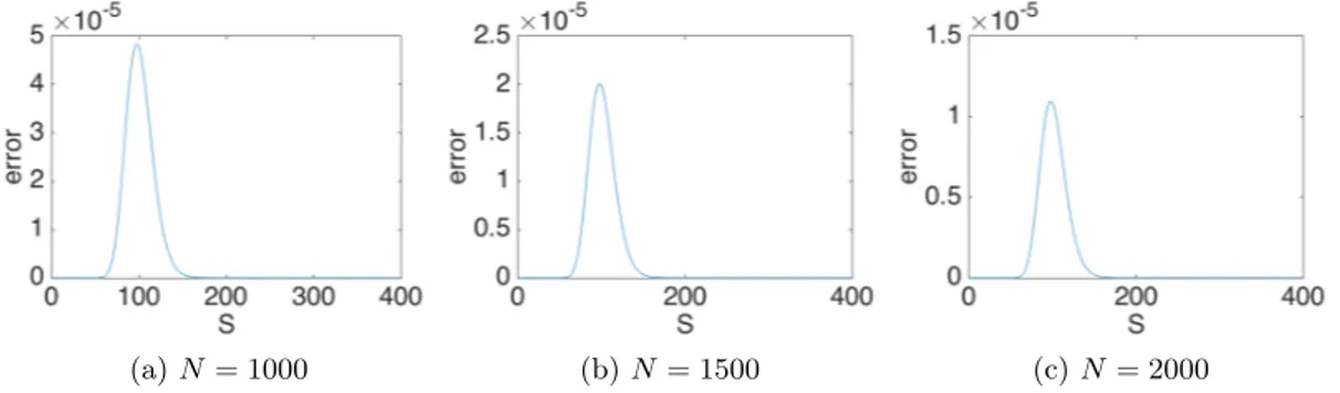
The fourth order Finite Diﬀerence scheme is run with the original nonsmooth pay oﬀ. As previously, the number of time steps is set to M = 20000.

(a) N = 1000 (b) N = 1500 (c) N = 2000

(15)

Figure 5: Logarithmic plot of maximum error as a function spatial grid size In Figure 4 the error over the space domain is shown for diﬀerent grid sizes, N = 1000, 1500, 2000. In Figure 5 a convergence plot is shown for the measured maximum error. As can be seen in Figure 4 the error is dominant around the strike price and decreasing for finer grids. In Figure 5 the convergence is estimated to 2.

(16)

7.3 Fourth order Finite Diﬀerence scheme on already smooth ini-tial condition

To measure the order of convergence on an already smooth initial conditions we set the initial condition to the analytical solution of the Black Scholes equation for t = T /2. The initial condition, u(T/2), is provided together with the actual pay oﬀ in Figure 6.

(a) The smooth initial condition (U0_{= U} a(T /2))

and the pay oﬀ function (b) Initial condition zoomed in around the strikeprice

Figure 6: The smooth initial condition

The simulation is then run until t = T for diﬀerent space grid sizes.

(a) N = 1000 (b) N = 1500 (c) N = 2000

(17)

Figure 8: Logarithmic plot of maximum error as a function spatial grid size In Figure 7 the error is shown over the space domain for diﬀerent grid sizes, analogical to section 6.2. In the same way a convergence plot is shown in Figure 8 with the measured values. The convergence for the already smooth initial condition is measured to 3.7. However, a error emerges near the right boundary, this error is constant regardless of the number of space steps.

(18)

7.4 Fourth order Finite Diﬀerence scheme on smoothed initial condition

Now we let the initial condition be the smoothed pay oﬀ function. In Figure 9 the smoothed initial condition is shown together with the pay oﬀ function.

(a) Smoothing of the pay oﬀ function (b) Smoothing zoomed in around strike price

Figure 9: The payoﬀ function before and after the smoothing of the initial condi-tion, to the right is a close up on the strike price

(a) N = 1000 (b) N = 1500 (c) N = 2000

(19)

Figure 11: Logarithmic plot of maximum error as a function spatial grid size In Figure 10, the error in space domain is shown for diﬀerent number of space grid steps. As in Section 6.3, the error around the strike price decreases with a convergence rate of order 4.2. However the same error as previously seen, close to the right boundary, is constant independently of the number of space steps.

8 Discussion

As can be seen in the result section we have second order of convergence for the second order Finite Diﬀerence scheme.

It can also be seen that the order of convergence for the nonsmooth initial condition is 2 even though the scheme is of fourth order. This is according to theory.

The fourth order scheme shows a fourth order of convergence between a very specific amount of grid sizes. The error around pay oﬀ continues to converge with order 4 but a error from the boundary gets dominant.

This error is probably due to our Finite Diﬀerence scheme, since it occurs for both smooth and smoothed initial conditions. It is probably caused by our strong implementation of the first inner boundary points and in further studies, a skew matrix with backward and forward Finite Diﬀerences for the first inner points should be used instead.

(20)

9 Conclusion

In order to investigate how the order of convergence is dependent on smoothness of the initial conditions when solving the Black Scholes equation with higher order of Finite Differences two Finite Difference schemes of second and fourth order were implemented. The second order scheme shows second order convergence regardless of the smoothness of the initial condition. The fourth order scheme does not show a fourth order convergence without smoothing of the initial condition. However, when the smoothing algorithm is implemented the results show that the fourth order scheme gives a convergence order of four and thus the smoothing algorithm works. It can be concluded that when fourth order Finite Difference schemes are used, a smooth initial conditions is necessary to show correct convergence.

(21)

10 References

Heston and Zhou, On the rate of convergence of discrete-time contingent claims, Mathematical Finance, Vol. 10, No. 1, (January 2000)

Kreiss, Thomée and Widlund, Smoothing of Initial Data and Rates of Conver-gence for Parabolic Diﬀerence Equations, Communications on pure and applied mathematics, Vol. XXIII, 241-259, (1970)

Tangman and Buruth, Numerical pricing of options using high-order compact fi-nite diﬀerence schemes, Journal of Computational and Applied Mathematics, 218, (2008)

Düring and Heuer, High-order compact schemes for parabolic problems with mixed derivatives in multiple space dimensions, SIAM Journal on Numerical Analysis 53:5, 2113-2134, (2015)

Hirsa, Computational Methods in Finance, London: Chapman & Hall/CRC Fi-nancial Mathematics Series, (2013)

Björk, Arbitrage Theory in Continuous Time, Third Edition, Oxford University Press, (2009)

(22)

11 Appendix

Matlab 2015

11.1 Second order cd_scheme

s=x; ds=dx; sigma=sig; gamma=1; alpha=0.5*sigma^2*s.^2/(ds^2); beta=0.5*r*s/ds; l=beta-alpha; d=r+2*alpha; upper=-(alpha+beta); cd_scheme=diag(d)+diag(l(2:end),-1)+diag(upper(1:end-1),1); cd_scheme(1,:)=zeros(1,N);

cd_scheme(end,:)=zeros(1,N); W=cd_scheme;

11.2 Fourth order cd_scheme

s=x; ds=dx; sigma=sig; gamma=1; alpha=0.5*sigma^2*s.^2/(ds^2); beta=r*s/ds; l2=1/12*alpha-1/12*beta; l1=-4/3*alpha+2/3*beta; d=r+5/2*alpha; upper1=-4/3*alpha-2/3*beta; upper2=1/12*alpha+1/12*beta; cd_scheme=diag(l2(3:end),-2)+diag(l1(2:end),-1)+diag(d)+... diag(upper1(1:end-1),1)+diag(upper2(1:end-2),2); cd_scheme(1,:)=zeros(1,N); cd_scheme(2,:)=zeros(1,N); cd_scheme(end-1,:)=zeros(1,N); cd_scheme(end,:)=zeros(1,N); W=cd_scheme;