We propose a new method to determine magnetic fields, by using the magnetic-field-induced electric dipole transition3p 3d4 4D7 2 3p5 2P3 2 in Fe9+ ions. This ion has a high abundance in astrophysical plasma and is therefore well suited for direct measurements of even rather weakfields in, e.g., solar flares. This transition is induced by an external magneticfield and its rate is proportional to the square of the magnetic field strength. We present theoretical values for what we will label the reduced rate and propose that the critical energy difference between the upper level in this transition and the close-to-degenerate3p 3d4 4D
5 2should be measured experimentally since it is required to determine the relative intensity of this magnetic line for different magneticfields.
Key words: atomic processes– Sun: corona – Sun: magnetic fields – Sun: UV radiation – techniques: spectroscopic
1. INTRODUCTION
One of the underlying causes behind solar events, such as solarflares, is the conversion of magnetic to thermal energy. It is therefore vital to be able to measure the magneticfield of the corona over hot active areas of the Sun that exhibit relatively strong magnetic fields. In order to follow the evolution of a solar flare, continuous observations are required, either from space or by using a network of ground-based instruments. It is therefore unfortunate that there are no space-based coronal magnetic field measurements, but only model estimates based on extrapolations from measurements of the photosphericfields (Schrijver et al. 2008). Ground-based measurements are performed either in the radio range (White 2004) across the solar corona or in the infrared wavelength range (Lin et al. 2004) on the solar limb. Infrared measurements of magnetic fields are limited by the fact that the spectral lines under investigation are optically thin. On the other hand, gyroreso-nance emission is optically thick, but refers only to a specific portion of the corona, which has a depth of around 100 km. From these measurements an absolutefield strength at the base of the corona, above active regions, in the range of 0.02–0.2 T was obtained(White & Kundu1997).
In this work we present a completely new method to measure magnetic fields of the active corona. This method is based on an exotic category of light generation, fed by the plasma magnetic field, external to the ions, in contrast to the internal fields generated by the bound electrons. The procedure relies on radiation in the soft X-ray region of the spectrum, implying a space-based method. This magnetic-field-induced radiation originates from atomic transitions where the lifetime of the upper energy level is sensitive to the local, external magnetic field (Beiersdorfer et al. 2003; Grumer et al. 2013, 2014; Li et al. 2013, 2014). We will show that there is a unique case where even relatively small external magneticfields can have a striking effect on the ion, leading to resonant magnetic-
field-induced light, due to what is called accidental degeneracy of quantum states.
The impact of the coronal magneticfield on the ion is usually very small due to the relative weakness of these fields in comparison to the strong internalfields of the ions. The effect therefore usually only contributes very weak lines that are impossible to observe. However, sometimes the quantum states end up very close to each other in energy, they are accidentally degenerate, and the perturbation by the external field will be enhanced. If this occurs with a state that without thefield has no, or only very weak, electromagnetic transitions to a lower state, a new and distinct feature in the spectrum from the ion will appear—a new strong line. Unfortunately, since the magnetic fields internal to the ion and the external fields generated in the coronal plasma differ by about five to seven orders of magnitude, the probability of a close-enough degeneracy is small. But in this report we will discuss a striking case of accidental degeneracy in an important ion for studies of the Sun and other stars, Fe9+.
The origin of the new lines in the spectra of ions is the breaking of the atomic symmetry by the external field, which will mix atomic states that have the same magnetic quantum number and parity. This will in turn introduce new decay channels from excited states(Andrew et al.1967; Wood et al. 1968), which we will label magnetic-field-induced transitions (MITs) (Grumer et al.2014). These transitions have attracted attention recently, when accurate and systematic methods to calculate their rates have been developed(Grumer et al.2013; Li et al.2013).
2. STRUCTURE OF CHLORINE-LIKE IONS AND MITS The structure of the lowest levels of chlorine-like ions is illustrated in Figure1. The important levels in the present study are the two lowest in the term 3p 3d4 4De, which turn out to
ignoring the effects of the nuclear spin, they both decay to the
P
3p5 2 o
3 2 level in the ground configuration, but while the
J=5 2has a fast electric dipole(E1) channel, the J=7 2can only decay via a slow magnetic quadrupole(M2) transition. In the presence of an external magnetic field, the two states will mix and induce a competing E1 transition channel (the MIT) from the J =7 2level. For most ions the M2 transition is still the dominant decay channel, but a crossing of thefine-structure levels D4
7 2and D4 5 2between cobalt and iron (see Figure2) will change the picture. As a matter of fact, for iron this fine-structure splitting energy is predicted to be at a minimum and the MIT contribution to the decay of the J =7 2level will be strongly enhanced.
Unfortunately, there are large variations in the predicted value of this energy difference (see Table 1). The aim of this report is therefore(a) to make a careful theoretical study of the energy splitting between the two 4De levels along the
isoelectronic sequence, to confirm the close degeneracy for iron, and(b) to make an accurate prediction of what we will label the reduced decay rate, aRMIT (see next section). This reduced rate can be combined with the experimentally determined wavelength and energy splitting to give the MIT rate for different magneticfields.
3. THEORETICAL METHOD AND COMPUTATIONAL MODEL
3.1. Theoretical Method
The basis of our theoretical approach is described in our earlier papers on MITs(Grumer et al.2013; Li et al.2013). In our example the reference state is 3p 3d4 4D
7 2ñ
∣ , which we can
represent by a mixture of two pure states in the presence of a magnetic field: D M d D M d M D M “3p 3d ” 3p 3d ( ) 3p 3d , (1) 4 4 7 2 0 4 4 7 2 1 4 4 5 2 = +
where we ignore interactions with other atomic states, since their energies are far from the reference state. The total E1 transition rate from a specific M sublevel in the mixed
D
“3p 3d4 4 7 2” to all the M′ sublevels of the ground level
P 3p5 2 3 2can be expressed as P A M A M M d M P D ( ) ( , ) 2.02613 10 3 ( ) 3p 3p 3d , (2) M MIT MIT 18 3 1 5 2 3 2 (1) 4 4 5 2 2
å
l = ¢ » ´ ´ ¢ whereλ is the transition wavelength and d M1( )depends on the magnetic quantum number M of the sublevels belonging to the
Figure 1. Schematic energy-level diagram for chlorine-like ions with Z < 26and zero nuclear spin, where D4
7 2is the lowest level in the configuration 3s 3p 3d2 4 .
For ions with Z > 26, a level crossing has occurred and D4
5 2 is lower than D
4
7 2. Under the influence of an external magnetic field, an E1 transition opens up
from the D4
7 2to the ground state through mixing with the D4 5 2.
Figure 2. Fine-structure splitting energy E E(4D ) E(D )
7 2 4 5 2
D = - as a
function of the nuclear charge, along the isoelectronic sequence from calculations reported here. The dashed line in green marksD = .E 0
Table 1 Atomic Data for FeX
Method λ DE AE1
Observation Solar(Thomas et al. 1994; Brosius et al.1998) 257.25 0 L Solar(Sandlin1979) L 5 L Theory Present 257.7285 20.14 6.30[6] MCDF(Huang et al.1983) 246.4924 78 1.63[6] MCDF(Dong et al.1999) 256.674 108 6.27[6] MCDF(Aggarwal & Keenan2004) L 54.85 L MR-RMBPT(Ishikawa et al.2010) 257.1924 18 L R-matrix(Del Zanna
et al.2012) 246.8890 109.74 L CI(Bhatia & Doschek1995) 256.1974 −58 1.21[6] CI(Deb et al.2002) 257.0846 21 2.42[5] Notes. List of the wavelengths λ (in Å) of the magnetically induced
D P
3p 3d4 4 3p
7 2 5 23 2 transition, the fine-structure splitting D =E
(
)
(
)
E 4D E D
5 2 - 4 7 2 (in cm−1), and the rate AE1(3p 3d4 4D5 23p5 2P3 2)
of the E1 transition(in s−1) for chlorine-like iron. The second column lists the various sources. x[n] indicates x × 10n.
D
3p 3d4 4
7 2level. For the3p 3d4 4D7 2level, d M1( )is given by
(
)
(
)
(
)
(
)
N N d M D M H D M E D E D B M D D E D E D ( ) 49 4 63 . (3) m 1 4 5 2 4 7 2 4 7 2 4 5 2 2 4 5 2 (1) (1) 4 7 2 4 7 2 4 5 2 = -= - - + D - As a result, the total rates of the3p 3d4 4D 3p P
7 2 5 23 2MITs from individual sublevels can be expressed as
A M a M B E ( ) ( ) ( ) , (4) R MIT MIT 2 3 2 l = D
where B is in units of T, λ is in units of Å,
(
)
(
)
E E 4D7 2 E 4D5 2
D = - is in units of cm−1, and we have
defined a reduced transition rate as
(
)
N N P a M M D D P D ( ) 2.02613 10 49 4 189 . (5) R MIT 18 2 4 5 2 (1) (1) 4 7 2 3 3 2 (1) 4 5 2 2 » ´ -´ + D The reduced rate defined in this equation is independent of the transition wavelength, the magneticfield strength as well as the energy splitting. This gives us the property that relates the MIT rates to the external magnetic field strength. To determine AMIT(M), we recommend to use theoretical values of aMITR (M), as reported in this work, combined with experimental values of the energy splitting and wavelength.
3.2. Correlation Model
The calculations are based on the multiconfiguration Dirac– Hartree–Fock method, in the form of the latest version of the GRASP2K program(Jönsson et al. 2013). A single reference configuration model is adopted for the even-parity (3p43d) and odd-parity (3p5) states, and the 1s, 2s, 2p core subshells are kept closed. The set of configuration state functions (CSFs) is
obtained by single and double excitations from the n= 3 shell of the reference configurations to the active set. The active set is augmented layer by layer to n = 7 (lmax=4) when satisfactory convergence is achieved. For each step, we optimize only the orbitals in the last added correlation layer at the time. In thefinal calculations, the total number of CSFs was 16,490 for the odd-parity(J = 3/2, 1/2) case and 523,421 for the even-parity(J = 1/2, 3/2, 5/2, 7/2, 9/2) case.
The resulting excitation energies of the 4D
7 2 and 4D5 2 change by less than 0.1% in the last step of the calculation. The final excitation energies agree with experiment to within 1%. The crucial energy splitting between D4
7 2 and D4 5 2 is well converged, except for iron where the close degeneracy occurs. To better represent this critical case we extended the calculations to include single excitations from the 2s and 2p subshells.
4. RESULTS AND DISCUSSION 4.1. Isoelectronic Sequence
We present in Table2all the important properties, according to Equation(4), involved in computing the MIT rates, i.e., the reduced transition rate aMITR (M), the energy splitting, D ,E between the two levels3p 3d4 4D
5 2and D4 7 2, together with the wavelength,λ, of the3p 3d4 4D 3p P
7 2 5 2 3 2transition. In the absence of an external magnetic field, magnetic quadrupole (M2) is the dominant decay channel for the
D P
3p 3d4 4 3p
7 2 5 23 2transition. When an external magnetic field is introduced, an additional decay channel is opened and
we define a average transition rate AMIT of the
D P 3p 3d4 4 7 23p5 23 2transition, A A M J ( ) 2 1 . (6) M MIT MIT
å
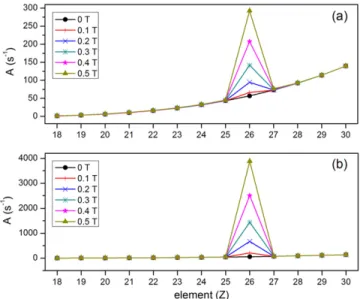
= +Rates for anyfield can be obtained from Equations (4) and (5). We plot the transition rates A = AM 2 + AMITalong the isoelectrionic sequence in Figure3(a) for some magnetic field strengths andDE = 20.14 cm-1for iron. It is clear that the magnetic field influences the transition rate substantially for
Cu 1.14[2] 1.309[1] 1.090[1] 6.543[0] −932.75 208.1047
Zn13+ 1.40[2] 1.347[1] 1.123[1] 6.736[0] −1482.74 195.3790
Notes. List of the M2 transition rates, AM2(in s−1), the reduced transition rate a (M)
R
MIT (in 10
12
cm T s
3 -2 -2 -1
Å ), and the wavelength λ (in Å) of the MIT transition
D P
3p 3d4 4 3p
iron due to the close degeneracy. To further illustrate the resonance behavior of this effect, we also used an astrophysical value(Sandlin1979) ED = 5 cm-1for iron, in Figure3(b).
4.2. FeX
Due to the close to complete cancellation for iron of the energy difference between the two D4 levels(see Figure2) we will pay special attention to this ion.
It is clear that some of the properties in Table2are more easily obtainable through theoretical calculations. We illustrate this in Table 3 where we show the convergence of the calculated off-diagonal reduced matrix elements, W = 4D N
5 2 (1)
á +
N(1) 4D
7 2
D ñ, representing the magnetic interaction, together
with the line strength,S 3P P D
3 2 (1) 4 5 2 2
= á ñ , of the
close-lying E1 transition. Since these values converge fast and are not subjected to cancellation effects, we estimate their accuracy to be well within a few per cent. This will in turn imply that the prediction of the reduced transition rate aMITR (M)in Equations(4) and(5) is of similar accuracy.
We give in Figure4the energy differenceD as a functionE
of the maximum n in the active set and thereby of the size of the CSF expansion. It is clear that we also here reach a
convergence close to a few cm−1 for this property. The final value for the fine-structure splitting is 20.14 cm−1, in good agreement with the result from recent configuration interaction calculations (Deb et al. 2002) as well as many-body perturbation theory (Ishikawa et al. 2010). This strongly supports the prediction of the close degeneracy of the two levels for iron.
The strong resonance effect for iron is especially fortunate due to its high abundance in many astrophysical plasmas. As a matter of fact, the ground transition is one of the “coronal” lines used to determine the temperature of the corona and is known as the corona red line (Swings 1943). Unfortunately there is no firm experimental value for the critical energy splitting between the D4
7 2and D4 5 2. At the same time, it is a great challenge to calculate the size of this accidental degeneracy accurately.
In the early experimental work by Smitt (1977) the two levels were given identical excitation energies of 388,708 cm−1. Since then there has been a great deal of work by different groups to study the structure of Fe X (see Table 1). The differences between the various calculations are often much larger than the predictedfine-structure splitting, which leads to large uncertainties in the level ordering and line identifications. Huang et al. (1983) and Dong et al. (1999) performed a multiconfiguration Dirac–Hartree–Fock (MCDHF) calculation and predicted the D4
5 2,7 2 levels to be separated by 78 and 108 cm−1 respectively. Ishikawa et al. (2010) predicted 18 cm−1from their Multireference–MBPT method. There is a recommended value from solar observations of around 5 cm−1, determined from short-wavelength transitions from higher levels and therefore probably quite uncertain. Predictions from the Goddard Solar Extreme Ultraviolet Rocket Telescope and Spectrograph SERTS-89 (Thomas & Neupert 1994) and SERTS-95(Brosius et al.1998) spectra give the same energy for D4 7 2and D4 5 2, probably due to limited resolution. Finally Del Zanna et al.(2004) benchmarked the atomic data for FeX and suggested the best splitting energy to be 5 cm−1. Although our calculations reach a convergence within the model, to the final value of around 20 cm−1, it is clear that systematic errors, such as omitted contributions to the Hamiltonian, could be relatively important in estimating the accidental degeneracy of
Figure 3. Total transition rate A = AM2 + AMIT of the 3p 3d4 4D7 2 P
3p5 2
3 2transition along the Cl-like isoelectronic sequence for some magnetic
field strengths. We used fine-structure energies of (a) 20.14 cm–1and(b) 5 cm−1
for iron.
Table 3
Convergence Study of the Calculations
Layer W S DF 0.5305 4.063[4] n= 4 0.5285 3.555[4] n= 5 0.5284 3.355[4] n= 6 0.5283 3.298[4] n= 7 0.5283 3.264[4]
Notes. Convergence study of calculated off-diagonal reduced matrix elements W= 4D N N D
5 2 (1) (1) 4 7 2
á + D ñ(in AU) of the magnetic interaction and line strength S = 3P P D
3 2 (1) 4 5 2 2
á ñ (in AU). DF represents a single configuration Dirac–Hartree–Fock model. x[n] indicates x´10n.
Figure 4. Convergence trend of the fine-structure separation
E E(4D ) E(D )
5 2 4 7 2
D = - for Fe9+as the size of the active set of orbitals
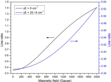
the two levels. We use both our theoretical value and the recommended solar spectral value to illustrate the dependence of the average rate AMITon the magneticfield in Figure5. It is clear that even for relatively weak magneticfields of only a few hundreds or thousands of gauss, AMIT will be significant compared to the competing M2 rate.
4.3. Experimental Determination of the Energy Splitting To improve the accuracy of the estimated rate of the MIT, we need to turn to experiment for an accurate determination of the energy splitting. For this, we need to overcome two difficulties: first, enough spectral resolution, and second, a light source with a low electron density and a magnetic field. The first requirement is not impossible to fulfill since the fine-structure separation can be determined using a large spectro-meter with a resolution of around 80,000. This is far from the highest resolution achieved, since, e.g., a spectrometer at the Observatory in Meudon has a resolution of 150,000. However, the line from the D4
7 2level has not been observed due to strict requirements on the light source. Most sources used at Meudon have generated too dense plasmas in which photon transitions from long-lived levels cannot be seen (collisions destroy the population of the upper state before the photon is emitted). In addition to this, observation of the D4 7 2 2P3 2line requires a strong enough magneticfield of, say, a tenth of a tesla. This leads arguably to only two possible light sources on Earth: tokamaks(Wesson2004) and electron beam ion traps (EBITs) (Levine et al. 1988). Tokamak plasma may be too dense, but since the magneticfields involved are higher than what we are discussing here, the line might still be observable. However, the best choice for our purposes is an EBIT, which has an inherent magneticfield to compress the electron beam and is a low-density light source. Although the Meudon spectrometer demonstrates that the required resolving power can be achieved, this instrument is not compatable with the EBIT operating parameters and a dedicated instrument is required.
To illustrate the usability of the EBIT source, we have made several model calculations to predict the relative strength of the two involved transitions under different circumstances. It
should be made clear that the EBIT is a light source with a monoenergetic beam of electrons and that these models therefore are designed to predict conditions different from those in solarflares or the corona. It is important to remember that the intermediate goal before we can proceed is to propose an experiment to determine the crucial D4 D
7 2-4 5 2 energy separation. We present model calculations of the line ratio as a function of magneticfield and electron density (Figure6) and magnetic field (Figure 7) of the EBIT, based on collisional-radiative modeling using the Flexible Atomic Code(Gu2008). We show in Figure6, for several magneticfields, how the ratio of the rates of the magnetic-field-induced D4 7 22 P3 2and the
allowed D4 P
5 22 3 2 transitions varies as a function of the electron densities. It is clear that the magnetic-field-induced line is predicted to be visible for the typical range of electron
Figure 5. Total average MIT rate, AMITdefined in Equation (6) plotted as a
function of magneticfields between 100 and 2000 gauss, at ΔE = 20.14 cm−1 andΔE = 5 cm−1, compared to the M2 transition rate, AM2.
Figure 6. Ratio of the rates for the magnetically induced D4 P 7 2 23 2line
and the allowed D4 P
5 2 23 2 line as a function of electron density and
magneticfield in an EBIT. Calculations are for a monoenergetic beam energy of 250 eV and these data are displayed for some selected magnetic field strengths and over a range of densities(10 –10 cm8 11 -3) that covers the range
for solarflares in the corona. Here we used the fine-structure energy of 5 cm−1.
Figure 7. Ratio of rates for the magnetically induced and the allowed transitions as a function of magnetic field in an EBIT. The model is for a monoenergetic electron beam energy of 250 eV and density of 1.0 ´ 10 cm11 -3.
densities of an EBIT, that is 10 –108 11cm-3 (this happens to coincide with the range for solar flares). It is also clear from Figure 7, where we show the dependence of this ratio on the magnitude of the external magnetic field for a fixed density of 1011cm-3, that the line ratio will be sensitive to the magnetic field strength.
5. CONCLUSION
To conclude, in this paper we propose a novel and efficient tool to determine magnetic field strengths in solar flares. The method is useful for cases of low densities and small external magneticfields (hundreds and thousands of gauss) that have so far eluded determination. We illustrate that a spectral feature originating from the Fe9+ ion is of special interest since it shows a strong dependence on the magneticfield strength, with two spectral lines drastically changing their relative intensities. We propose a laboratory measurement of the fine-structure energy separation between the two involved excited states, a crucial parameter in the determination of the external field. When this energy separation has been established one can use our theoretical values for the reduced rate of the MIT, which have an accuracy to within a few per cent, to calculate the atomic response to the external magneticfield. Armed with this it is possible to design a space-based mission with a probe that could continuously observe and determine the reclusive magnetic fields of solar flares.
This work was supported by the Chinese National Fusion Project for ITER No. 2015GB117000, Shanghai Leading Academic Discipline Project No. B107. We also gratefully acknowledge support from the Swedish Institute under the Visby programme. W.L. and J.G. would like to especially
thank the Nordic Centre at Fudan University for supporting their visits between Lund and Fudan Universities.
REFERENCES
Aggarwal, K. M., & Keenan, F. P. 2004,A&A,427, 763
Andrew, K. L., Cowan, R. D., & Giacchetti, A. 1967,JOSA,57, 715 Beiersdorfer, P., Scofield, J. H., & Osterheld, A. L. 2003,PhRvL,90, 235003 Bhatia, A., & Doschek, G. 1995,ADNDT,60, 97
Brosius, J., Davila, J., & Thomas, R. 1998,ApJS,119, 255 Deb, N. C., Gupta, G. P., & Msezane, A. Z. 2002,ApJS,141, 247 Del Zanna, G., Berrington, K. A., & Mason, H. E. 2004,A&A,422, 731 Del Zanna, G., Storey, P. J., Badnell, N. R., & Mason, H. E. 2012,A&A,
541, A90
Dong, C. Z., Fritzsche, S., Fricke, B., & Sepp, W.-D. 1999, MNRAS, 307, 809
Grumer, J., Brage, T., Andersson, M., et al. 2014,PhyS,89, 114002 Grumer, J., Li, W., Bernhardt, D., et al. 2013,PhRvA,88, 022513 Gu, M. F. 2008,CaJPh,86, 675
Huang, K.-N., Kim, K., & Cheng, K. T. 1983,ADNDT,28, 355 Ishikawa, Y., Santana, J. A., & Trabert, E. 2010,JPhB,43, 074022 Jönsson, P., Gaigalas, G., Biero, J., Fischer, C. F., & Grant, I. 2013,CoPhC,
184, 2197
Levine, M. A., Marrs, R. E., Henderson, J. R., Knapp, D. A., & Schneider, M. B. 1988, PhyS, T22, 157
Li, J., Brage, T., Jönsson, P., & Yang, Y. 2014, arXiv:1405.7787v1 Li, J., Grumer, J., Li, W., et al. 2013,PhRvA,88, 013416 Lin, H., Kuhn, J. R., & Coulter, R. 2004, ApL, 613, L177 Sandlin, G. D. 1979,ApJ,227, L107
Schrijver, C. J., DeRosa, M. L., Metcalf, T., et al. 2008,ApJ,675, 1637 Smitt, R. 1977, SoPh,51, 113
Swings, P. 1943,ApJ,98, 116
Thomas, R., & Neupert, W. 1994,APJS,91, 461
Wesson, J. 2004, Tokamaks(3rd ed.; New York: Oxford Univ. Press) White, S. M. 2004, in Solar and Space Weather Radiophysics, ed. D. E. Gary &
C. U. Keller(Berlin: Springer), 89
White, S. M., & Kundu, M. R. 1997,SoPh,174, 31
Wood, D. R., Andrew, K. L., Giacchetti, A., & Cowan, R. D. 1968,JOSA, 58, 830