ScienceDirect
Available online at www.sciencedirect.com
Procedia Computer Science 113 (2017) 502–507
1877-0509 © 2017 The Authors. Published by Elsevier B.V. Peer-review under responsibility of the Conference Program Chairs. 10.1016/j.procs.2017.08.312
10.1016/j.procs.2017.08.312
© 2017 The Authors. Published by Elsevier B.V.
Peer-review under responsibility of the Conference Program Chairs.
1877-0509 Available online at www.sciencedirect.com
Procedia Computer Science 00 (2017) 000–000
www.elsevier.com/locate/procedia
The 2nd edition of the International Workshop on Data Mining on IoT Systems (DaMIS)
Prediction of bicycle counter data using regression
Johan Holmgren
a,b,∗, Sebastian Aspegren
a, Jonas Dahlström
aaDepartment of Computer Science and Media Technology, Malmö University, Malmö 205 06, Sweden bK2 (The Swedish Knowledge Centre for Public Transport)
Abstract
We present a study, where we used regression in order to predict the number of bicycles registered by a bicycle counter (located in Malmö, Sweden). In particular, we compared two regression problems, differing only in their target variables (one using the absolute number of bicycles as target variable and the other one using the deviation from a long-term trend estimate of the expected number of bicycles as target variable). Our results show that using the trend curve deviation as target variable has potential to improve the prediction accuracy (compared to using the absolute number of bicycles as target variable). The results also show that support vector regression (using 2nd and 3rd degree polynomial kernels) and regression trees perform best for our problem.
c
�2017 The Authors. Published by Elsevier B.V.
Peer-review under responsibility of the Conference Program Chairs.
Keywords: Bicycle counter, regression, trend curve, regression algorithm comparison
1. Introduction
The bicycle has become an important part of urban transport due to its ability to contribute to fast, sustainable, and cost efficient transport. It also contributes to a healthy, active, life style, and the popularity of the bicycle is accentuated by the increase of bicycling that can be observed around the world. Due to the positive effects of bicycling, there is an increasing interest from public authorities to increase the use of the bicycle. However, in order to achieve a modal shift towards bicycling (from motorized transport), it is important to increase the attractiveness of the bicycle. This can be achieved by implementing various types of policy measures, including the construction and improvement of biking infrastructure, such as bicycling lanes and safe parking facilities. Other initiatives include bicycle sharing systems, which are currently being implemented in cities around the world1,2. Bicycle sharing systems enable, for example,
fast multimodal passenger transport, where public transport and the bicycle can be combined in an efficient way1. The
recent introduction of electrical bicycles, is another factor that increases the attractiveness of the bicycle3.
However, in order to build a transport system that encourages bicycling, it is important to fully understand the current bicycle flows, and what factors influence the travelers’ choices whether to travel by bicycle, to use some other mode of transport (e.g., car or bus), or to not travel at all. Hence, it is important to collect various types of traffic, transport and bicycle related data, which can be done using Internet of Things (IoT) connected devices, such as bicycle
∗Corresponding author. Tel.: +46-40-6657688 ; fax: +46-40-665 76 46.
E-mail address:johan.holmgren@mah.se
1877-0509 c�2017 The Authors. Published by Elsevier B.V. Peer-review under responsibility of the Conference Program Chairs.
Available online at www.sciencedirect.com
Procedia Computer Science 00 (2017) 000–000
www.elsevier.com/locate/procedia
The 2nd edition of the International Workshop on Data Mining on IoT Systems (DaMIS)
Prediction of bicycle counter data using regression
Johan Holmgren
a,b,∗, Sebastian Aspegren
a, Jonas Dahlström
aaDepartment of Computer Science and Media Technology, Malmö University, Malmö 205 06, Sweden bK2 (The Swedish Knowledge Centre for Public Transport)
Abstract
We present a study, where we used regression in order to predict the number of bicycles registered by a bicycle counter (located in Malmö, Sweden). In particular, we compared two regression problems, differing only in their target variables (one using the absolute number of bicycles as target variable and the other one using the deviation from a long-term trend estimate of the expected number of bicycles as target variable). Our results show that using the trend curve deviation as target variable has potential to improve the prediction accuracy (compared to using the absolute number of bicycles as target variable). The results also show that support vector regression (using 2nd and 3rd degree polynomial kernels) and regression trees perform best for our problem.
c
�2017 The Authors. Published by Elsevier B.V.
Peer-review under responsibility of the Conference Program Chairs.
Keywords: Bicycle counter, regression, trend curve, regression algorithm comparison
1. Introduction
The bicycle has become an important part of urban transport due to its ability to contribute to fast, sustainable, and cost efficient transport. It also contributes to a healthy, active, life style, and the popularity of the bicycle is accentuated by the increase of bicycling that can be observed around the world. Due to the positive effects of bicycling, there is an increasing interest from public authorities to increase the use of the bicycle. However, in order to achieve a modal shift towards bicycling (from motorized transport), it is important to increase the attractiveness of the bicycle. This can be achieved by implementing various types of policy measures, including the construction and improvement of biking infrastructure, such as bicycling lanes and safe parking facilities. Other initiatives include bicycle sharing systems, which are currently being implemented in cities around the world1,2. Bicycle sharing systems enable, for example,
fast multimodal passenger transport, where public transport and the bicycle can be combined in an efficient way1. The
recent introduction of electrical bicycles, is another factor that increases the attractiveness of the bicycle3.
However, in order to build a transport system that encourages bicycling, it is important to fully understand the current bicycle flows, and what factors influence the travelers’ choices whether to travel by bicycle, to use some other mode of transport (e.g., car or bus), or to not travel at all. Hence, it is important to collect various types of traffic, transport and bicycle related data, which can be done using Internet of Things (IoT) connected devices, such as bicycle
∗Corresponding author. Tel.: +46-40-6657688 ; fax: +46-40-665 76 46.
E-mail address:johan.holmgren@mah.se
1877-0509 c�2017 The Authors. Published by Elsevier B.V. Peer-review under responsibility of the Conference Program Chairs.
2 Holmgren et al. / Procedia Computer Science 00 (2017) 000–000
counters and mobile phone applications that enables registering the movement of travellers. Bicycle counters, which are the focus of the current paper, allow to continuously register the bicycles that pass some particular point in a transport network. Due to the possibility to register a large share of the passing bicycles, bicycle counters (typically built using inductive loop detectors) are commonly used to collect bicycle flow data.
In the presented study, we analyzed data collected by a bicycle counter located in Malmö, Sweden. An important purpose of our work was to quantify how various factors, such as day of week, time of year, and weather (temperature and precipitation), is expected to influence the amount of bicycle traffic at a particular point in the traffic network. We studied how it is appropriate to formulate a regression problem that can be used to estimate the number of bicycles registered by a bicycle counter. In particular, we investigated whether the use of a long-term trend estimate of the number of registered bicycles has the potential to improve the regression accuracy. We also compared different regression approaches, in order to identify which approach is most suitable for the considered problem. The current study builds on the Bachelor’s thesis of Aspegren and Dahlström4, who compared a set of regression algorithms
regarding their ability to estimate the number of bicycles registered by our bicycle counter. Aspegren and Dahlström limited their analysis to consider only working days, whereas we include all days in the regression problem, explicitly considering day of week, school breaks, national holidays, and bridge days as input features.
Our work aims to provide input for passenger transport analysis models used by city and transport planners, e.g., for assessing the impact of transport policy measures. The relevance in this direction is emphasized by the fact that bicycling is currently being incorporated in passenger transport analysis models.
The current paper is organized in the following way. In the next section we give an account to previous research related to our work. In Section 3, we describe the data processing that we conducted in the beginning of our study. In Section 4, we present our regression modeling, which is followed in Section 5 by our computational results. We finalize the paper in Section 6 with some conclusions and pointers to future work.
2. Related work
The research related to bicycle data analysis has been quite intensive during the recent years. Romanillos et al.5 provide an overview of big data approaches applied in the bicycling context. A large amount of research concern bicycle sharing systems, where the studied problems include bicycle repositioning6and location of base (or docking) stations7. Data mining has been applied in the bicycle sharing context, for example, in order to estimate usage patterns8,9. Data mining also plays an important role in travel demand estimation (including bicycle demand analysis),
which is an integral part of traffic and transport analysis models (both in urban and in regional contexts). Traditionally, travel demand is estimated using travel survey data, often combined with GPS trajectories10. Bicycle demand can be
further estimated using different types of discrete choice models, which have been used, for example, for bicycle route and destination choice estimations11. In addition, there exists research on how various factors, including weather,
calendar events, and work related factors, influence the choice whether or not to use the bicycle12,13.
The current paper focus on regression analysis using bicycle counter data in order to quantify how factors such as weather are expected to influence the amount of bicycling. According to the best of our knowledge, there exist no such previous study, except for the work by Aspegren and Dahlström4.
3. Data pre-processing
In our study, we considered the time period September 13, 2006 to March 31, 2014, where we used bicycle volume data from a bicycle counter located in the city center of Malmö, weather data (i.e., temperature and precipitation), and information about national holidays and school breaks. We obtained information about school breaks from the web pages of the public schools in Malmö; however, as complete information about school breaks were not publicly available for the considered time period, we made a few assumptions concerning school breaks. In particular, we assumed that the longer school breaks occur during the same weeks each year, which was partially confirmed by the municipality of Malmö. The bicycle counter and weather data sets, which we received from the municipality of Malmö, specify values hourly. However, in the regression problem, where we considered each day as a data point, we aggregated the bicycle counter data for each day, and we used the averages of the temperature and precipitation values for each day. In addition, the bicycle counter and weather data sets had some missing values, which we estimated
Procedia Computer Science 00 (2017) 000–000
www.elsevier.com/locate/procedia
The 2nd edition of the International Workshop on Data Mining on IoT Systems (DaMIS)
Prediction of bicycle counter data using regression
Johan Holmgren
a,b,∗, Sebastian Aspegren
a, Jonas Dahlström
aaDepartment of Computer Science and Media Technology, Malmö University, Malmö 205 06, Sweden bK2 (The Swedish Knowledge Centre for Public Transport)
Abstract
We present a study, where we used regression in order to predict the number of bicycles registered by a bicycle counter (located in Malmö, Sweden). In particular, we compared two regression problems, differing only in their target variables (one using the absolute number of bicycles as target variable and the other one using the deviation from a long-term trend estimate of the expected number of bicycles as target variable). Our results show that using the trend curve deviation as target variable has potential to improve the prediction accuracy (compared to using the absolute number of bicycles as target variable). The results also show that support vector regression (using 2nd and 3rd degree polynomial kernels) and regression trees perform best for our problem.
c
�2017 The Authors. Published by Elsevier B.V.
Peer-review under responsibility of the Conference Program Chairs.
Keywords: Bicycle counter, regression, trend curve, regression algorithm comparison
1. Introduction
The bicycle has become an important part of urban transport due to its ability to contribute to fast, sustainable, and cost efficient transport. It also contributes to a healthy, active, life style, and the popularity of the bicycle is accentuated by the increase of bicycling that can be observed around the world. Due to the positive effects of bicycling, there is an increasing interest from public authorities to increase the use of the bicycle. However, in order to achieve a modal shift towards bicycling (from motorized transport), it is important to increase the attractiveness of the bicycle. This can be achieved by implementing various types of policy measures, including the construction and improvement of biking infrastructure, such as bicycling lanes and safe parking facilities. Other initiatives include bicycle sharing systems, which are currently being implemented in cities around the world1,2. Bicycle sharing systems enable, for example,
fast multimodal passenger transport, where public transport and the bicycle can be combined in an efficient way1. The
recent introduction of electrical bicycles, is another factor that increases the attractiveness of the bicycle3.
However, in order to build a transport system that encourages bicycling, it is important to fully understand the current bicycle flows, and what factors influence the travelers’ choices whether to travel by bicycle, to use some other mode of transport (e.g., car or bus), or to not travel at all. Hence, it is important to collect various types of traffic, transport and bicycle related data, which can be done using Internet of Things (IoT) connected devices, such as bicycle
∗ Corresponding author. Tel.: +46-40-6657688 ; fax: +46-40-665 76 46.
E-mail address:johan.holmgren@mah.se
1877-0509 c�2017 The Authors. Published by Elsevier B.V. Peer-review under responsibility of the Conference Program Chairs.
2 Holmgren et al. / Procedia Computer Science 00 (2017) 000–000
counters and mobile phone applications that enables registering the movement of travellers. Bicycle counters, which are the focus of the current paper, allow to continuously register the bicycles that pass some particular point in a transport network. Due to the possibility to register a large share of the passing bicycles, bicycle counters (typically built using inductive loop detectors) are commonly used to collect bicycle flow data.
In the presented study, we analyzed data collected by a bicycle counter located in Malmö, Sweden. An important purpose of our work was to quantify how various factors, such as day of week, time of year, and weather (temperature and precipitation), is expected to influence the amount of bicycle traffic at a particular point in the traffic network. We studied how it is appropriate to formulate a regression problem that can be used to estimate the number of bicycles registered by a bicycle counter. In particular, we investigated whether the use of a long-term trend estimate of the number of registered bicycles has the potential to improve the regression accuracy. We also compared different regression approaches, in order to identify which approach is most suitable for the considered problem. The current study builds on the Bachelor’s thesis of Aspegren and Dahlström4, who compared a set of regression algorithms
regarding their ability to estimate the number of bicycles registered by our bicycle counter. Aspegren and Dahlström limited their analysis to consider only working days, whereas we include all days in the regression problem, explicitly considering day of week, school breaks, national holidays, and bridge days as input features.
Our work aims to provide input for passenger transport analysis models used by city and transport planners, e.g., for assessing the impact of transport policy measures. The relevance in this direction is emphasized by the fact that bicycling is currently being incorporated in passenger transport analysis models.
The current paper is organized in the following way. In the next section we give an account to previous research related to our work. In Section 3, we describe the data processing that we conducted in the beginning of our study. In Section 4, we present our regression modeling, which is followed in Section 5 by our computational results. We finalize the paper in Section 6 with some conclusions and pointers to future work.
2. Related work
The research related to bicycle data analysis has been quite intensive during the recent years. Romanillos et al.5 provide an overview of big data approaches applied in the bicycling context. A large amount of research concern bicycle sharing systems, where the studied problems include bicycle repositioning6and location of base (or docking) stations7. Data mining has been applied in the bicycle sharing context, for example, in order to estimate usage patterns8,9. Data mining also plays an important role in travel demand estimation (including bicycle demand analysis),
which is an integral part of traffic and transport analysis models (both in urban and in regional contexts). Traditionally, travel demand is estimated using travel survey data, often combined with GPS trajectories10. Bicycle demand can be
further estimated using different types of discrete choice models, which have been used, for example, for bicycle route and destination choice estimations11. In addition, there exists research on how various factors, including weather,
calendar events, and work related factors, influence the choice whether or not to use the bicycle12,13.
The current paper focus on regression analysis using bicycle counter data in order to quantify how factors such as weather are expected to influence the amount of bicycling. According to the best of our knowledge, there exist no such previous study, except for the work by Aspegren and Dahlström4.
3. Data pre-processing
In our study, we considered the time period September 13, 2006 to March 31, 2014, where we used bicycle volume data from a bicycle counter located in the city center of Malmö, weather data (i.e., temperature and precipitation), and information about national holidays and school breaks. We obtained information about school breaks from the web pages of the public schools in Malmö; however, as complete information about school breaks were not publicly available for the considered time period, we made a few assumptions concerning school breaks. In particular, we assumed that the longer school breaks occur during the same weeks each year, which was partially confirmed by the municipality of Malmö. The bicycle counter and weather data sets, which we received from the municipality of Malmö, specify values hourly. However, in the regression problem, where we considered each day as a data point, we aggregated the bicycle counter data for each day, and we used the averages of the temperature and precipitation values for each day. In addition, the bicycle counter and weather data sets had some missing values, which we estimated
504 Johan Holmgren et al. / Procedia Computer Science 113 (2017) 502–507
Holmgren et al. / Procedia Computer Science 00 (2017) 000–000 3
using interpolation. Weather data values were missing up to a few hours here and there, and bicycle counter values were missing for periods up to a couple of weeks in either or both of the directions.
We estimated a missing weather factor value xhk for some hour hk, between two hours hiand hj(hi<hk<hj) with
known weather factor values as xhk = xhi+
xhj−xhi
hj−hi
(hk−hi) , (1)
where xhiand xhjdenote the (known) weather factor values for hours hiand hjrespectively. Similarly, we estimated a
missing bicycle counter value by taking the average of the corresponding hour one year immediately before and one year immediately after the missing values. For example, we estimated a missing bicycle counter value xh,d,w,yfor hour
hon weekday d in week w and year y as
xh,d,w,y=
xh,d,w,y−1+ xh,d,w,y+1
2 . (2)
4. Regression problem formulation
We formulated our regression problem, as an extension of the model by Aspegren and Dahlström4, using the
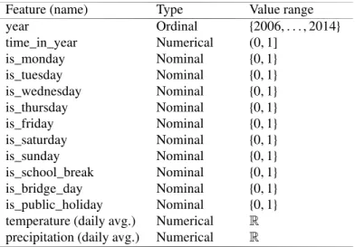
input features provided in Table 1. It should be mentioned that for the i:th day in a year, the time_in_year feature is calculated as ni, where n is the number of days in the year (either 365 or 366). For our set of input features, we formulated two regression problems (P1 and P2), which differ only in their target variables.
Table 1. Input features used in our two regression problems.
Feature (name) Type Value range
year Ordinal {2006, . . . , 2014} time_in_year Numerical (0, 1] is_monday Nominal {0, 1} is_tuesday Nominal {0, 1} is_wednesday Nominal {0, 1} is_thursday Nominal {0, 1} is_friday Nominal {0, 1} is_saturday Nominal {0, 1} is_sunday Nominal {0, 1} is_school_break Nominal {0, 1} is_bridge_day Nominal {0, 1} is_public_holiday Nominal {0, 1} temperature (daily avg.) Numerical R precipitation (daily avg.) Numerical R
As mentioned in Section 1, our purpose for using regression was to estimate the number of bicycles registered by a bicycle counter, considering the factors provided in Table 1. Therefore, we chose to use the total number of (daily) registered bicycles as regression target variable in one of our regression problems (P1). In P2, we instead used the deviation from an estimated long-term trend curve as target variable.
Our reason for formulating P2 was that we observed a long-term trend of varying number of registered bicycles at the bicycle counter. The diagram to the right in Fig. 1, which presents the moving yearly average of the number of registered bicycles per day, shows that we have an initial increase of bicycle volumes, followed by a decrease, and by another increase at the end of the time series. This contradicts what is expected, as there has been a rather linear increase of the population in Malmö from about 276000 as of December 31, 2006 to about 318000 as of December 31, 2014. This means that the number of bicycles registered by the counter, most likely does not follow the overall trend in Malmö. For example, the observed decrease might be partly due to the opening of a new railway station in 2010,
4 Holmgren et al. / Procedia Computer Science 00 (2017) 000–000
Fig. 1. Average number of bicycles per day using three week moving average (to the left) and yearly moving average (to the right).
resulting in a redistribution of the bicycle flows in Malmö. In order to consider this (probably) deviating trend at the bicycle counter, we decided to formulate our regression problem P2, where we used the deviation from a long-term trend estimate at the bicycle counter instead of the absolute number of bicycles as target variable.
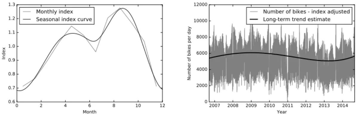
We constructed our trend estimate (or trend curve) using the following steps (see also Fig. 2):
1. We calculated monthly indices (over the number of bicycles) using the ratio-to-moving-average method, for which we estimated a seasonal index curve (using splines).
2. For each day, we divided the number of registered bicycles with the index given by the seasonal index curve. 3. Finally, we fitted a 4 degree polynomial to the index adjusted time series, giving us our long-term trend estimate.
Fig. 2. Monthly volume indices, seasonal index curve, and the long-term trend estimate that we used in our regression problem P2. For each day (d), the deviation from the long-term trend estimate (used as target variable in P2) is given by
num_bicyclesd−f(d)
f(d) , where f (d) is the number of bicycles given by the long-term trend estimate for day d.
5. Computational results
In order to compare the performance of different regression approaches, and to investigate whether the use of a long-term trend estimate has potential to improve the regression accuracy, we implemented and evaluated our regression problems (P1 and P2) using Weka (the Waikato Environment for Knowledge Analysis) machine learning tool14.
In our study, we included the following (six) regression algorithms:
using interpolation. Weather data values were missing up to a few hours here and there, and bicycle counter values were missing for periods up to a couple of weeks in either or both of the directions.
We estimated a missing weather factor value xhk for some hour hk, between two hours hiand hj(hi<hk<hj) with
known weather factor values as xhk = xhi+
xhj−xhi
hj−hi
(hk−hi) , (1)
where xhiand xhjdenote the (known) weather factor values for hours hiand hjrespectively. Similarly, we estimated a
missing bicycle counter value by taking the average of the corresponding hour one year immediately before and one year immediately after the missing values. For example, we estimated a missing bicycle counter value xh,d,w,yfor hour
hon weekday d in week w and year y as
xh,d,w,y=
xh,d,w,y−1+ xh,d,w,y+1
2 . (2)
4. Regression problem formulation
We formulated our regression problem, as an extension of the model by Aspegren and Dahlström4, using the
input features provided in Table 1. It should be mentioned that for the i:th day in a year, the time_in_year feature is calculated as ni, where n is the number of days in the year (either 365 or 366). For our set of input features, we formulated two regression problems (P1 and P2), which differ only in their target variables.
Table 1. Input features used in our two regression problems.
Feature (name) Type Value range
year Ordinal {2006, . . . , 2014} time_in_year Numerical (0, 1] is_monday Nominal {0, 1} is_tuesday Nominal {0, 1} is_wednesday Nominal {0, 1} is_thursday Nominal {0, 1} is_friday Nominal {0, 1} is_saturday Nominal {0, 1} is_sunday Nominal {0, 1} is_school_break Nominal {0, 1} is_bridge_day Nominal {0, 1} is_public_holiday Nominal {0, 1} temperature (daily avg.) Numerical R precipitation (daily avg.) Numerical R
As mentioned in Section 1, our purpose for using regression was to estimate the number of bicycles registered by a bicycle counter, considering the factors provided in Table 1. Therefore, we chose to use the total number of (daily) registered bicycles as regression target variable in one of our regression problems (P1). In P2, we instead used the deviation from an estimated long-term trend curve as target variable.
Our reason for formulating P2 was that we observed a long-term trend of varying number of registered bicycles at the bicycle counter. The diagram to the right in Fig. 1, which presents the moving yearly average of the number of registered bicycles per day, shows that we have an initial increase of bicycle volumes, followed by a decrease, and by another increase at the end of the time series. This contradicts what is expected, as there has been a rather linear increase of the population in Malmö from about 276000 as of December 31, 2006 to about 318000 as of December 31, 2014. This means that the number of bicycles registered by the counter, most likely does not follow the overall trend in Malmö. For example, the observed decrease might be partly due to the opening of a new railway station in 2010,
Fig. 1. Average number of bicycles per day using three week moving average (to the left) and yearly moving average (to the right).
resulting in a redistribution of the bicycle flows in Malmö. In order to consider this (probably) deviating trend at the bicycle counter, we decided to formulate our regression problem P2, where we used the deviation from a long-term trend estimate at the bicycle counter instead of the absolute number of bicycles as target variable.
We constructed our trend estimate (or trend curve) using the following steps (see also Fig. 2):
1. We calculated monthly indices (over the number of bicycles) using the ratio-to-moving-average method, for which we estimated a seasonal index curve (using splines).
2. For each day, we divided the number of registered bicycles with the index given by the seasonal index curve. 3. Finally, we fitted a 4 degree polynomial to the index adjusted time series, giving us our long-term trend estimate.
Fig. 2. Monthly volume indices, seasonal index curve, and the long-term trend estimate that we used in our regression problem P2. For each day (d), the deviation from the long-term trend estimate (used as target variable in P2) is given by
num_bicyclesd−f(d)
f(d) , where f (d) is the number of bicycles given by the long-term trend estimate for day d.
5. Computational results
In order to compare the performance of different regression approaches, and to investigate whether the use of a long-term trend estimate has potential to improve the regression accuracy, we implemented and evaluated our regression problems (P1 and P2) using Weka (the Waikato Environment for Knowledge Analysis) machine learning tool14.
In our study, we included the following (six) regression algorithms:
506 Johan Holmgren et al. / Procedia Computer Science 113 (2017) 502–507
Holmgren et al. / Procedia Computer Science 00 (2017) 000–000 5
• M5P (model tree where each leaf is an M5 rule). • Rep tree (regression tree built using information gain).
• Linear regression (linear regression function built using the Akaike metric). • Multi layer perceptron (network model based on back propagation).
• SMOReg (Support vector regression with 1,2, and 3 degree polynomial kernels).
We chose to include the three first algorithms as they were the most promising algorithms (for a similar regression problem) according to Aspegren and Dahlström4, and we included the remaining three algorithms in order to make the
set of selected algorithms more diverse. Even though some meta algorithms, such as Random subspace and Bagging, have potential to provide good accuracy4, we chose to not consider any meta algorithms in the current study. In
addition, tuning the selected algorithms (to optimize their performance) was outside the scope of the current study. For each of the selected algorithms, we constructed regression models (using 10-fold cross validation) for both P1 and P2. We then generated output metrics using the metrics package included in the scikit-learn machine learning library for Python. The reason for exporting the Weka output and further processing it using Python was that we needed to translate the predictions made for P2 into absolute number of bicycles, hence providing comparable metrics for our two regression problems.
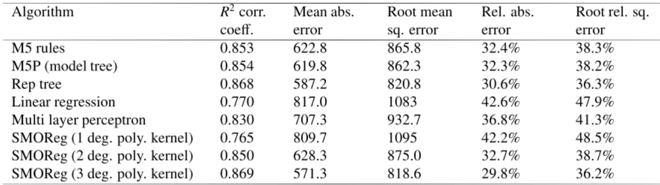
Our results (see Table 2 and Table 3) clearly indicate that, among the tested algorithms, SMO reg (support vector regression using 2nd and 3rd degree polynomial kernels) and Rep tree (regression tree) perform best for our regression problems. For each of the considered regression algorithms (except for Multi layer perceptron using the standard Weka configuration) our results also shows that all of the considered output metrics are better for P2 than for P1. That is, the problem where we used the deviation from the trend curve as target variable performs best.
Table 2. Results for regression problem P1, using the absolute number of registered bicycles as target variable.
Algorithm R2corr. coeff. Mean abs. error Root mean sq. error Rel. abs. error Root rel. sq. error M5 rules 0.853 622.8 865.8 32.4% 38.3% M5P (model tree) 0.854 619.8 862.3 32.3% 38.2% Rep tree 0.868 587.2 820.8 30.6% 36.3% Linear regression 0.770 817.0 1083 42.6% 47.9%
Multi layer perceptron 0.830 707.3 932.7 36.8% 41.3%
SMOReg (1 deg. poly. kernel) 0.765 809.7 1095 42.2% 48.5%
SMOReg (2 deg. poly. kernel) 0.850 628.3 875.0 32.7% 38.7%
SMOReg (3 deg. poly. kernel) 0.869 571.3 818.6 29.8% 36.2%
Table 3. Results for regression problem P2, using the deviation from the trend curve shown in Fig. 2 as target variable. The performance metrics corresponds to the absolute number of bicycles.
Algorithm R2corr. coeff. Mean abs. error Root mean sq. error Rel. abs. error Root rel. sq. error M5 rules 0.859 599.2 848.1 31.2% 37.5% M5P (model tree) 0.869 575.9 818.8 30.0% 36.2% Rep tree 0.875 563.8 799.2 29.4% 35.4% Linear regression 0.798 755.3 1015 39.3% 44.9%
Multi layer perceptron 0.826 695.1 943.5 36.2% 41.7%
SMOReg (1 deg. poly. kernel) 0.792 745.9 1031 38.9% 45.6%
SMOReg (2 deg. poly. kernel) 0.866 579.3 826.7 30.2% 36.6%
SMOReg (3 deg. poly. kernel) 0.871 559.8 810.6 29.2% 35.9%
6 Holmgren et al. / Procedia Computer Science 00 (2017) 000–000
6. Conclusions and future work
We have studied how regression can be used to estimate the number of bicycles registered by a bicycle counter (located in Malmö, Sweden). In particular, we formulated and compared two regression problems, which only differ in their target variables (one with the absolute number of bicycles as target variable and one with the deviation from a long-term trend estimate of the expected number of bicycles as target variable). In addition, we compared a number of regression algorithms (see Section 5) in order to find out which algorithms perform best for the considered problem.
For the two versions of our regression problem, we obtained the results presented in Table 2 and Table 3. In particular, it should be emphasized that, by explicitly modeling day of week, national holidays, school breaks, and bridge days as input features, we managed to significantly improve the prediction accuracy compared to the results recently obtained by Aspegren and Dahlström4. For example, in terms of relative absolute error, we managed to
improve the results from about 90% to around 30% for the best performing algorithms. This shows that it is important to consider input features representing different day characteristics in the regression problem formulation.
Our results show that using the deviation from the number of expected bicycles provided by a long-term trend estimate as target variable has potential to improve the prediction accuracy (compared to using the absolute number of bicycles as target variable). For example, for the relative absolute error, we observed an improvement from 29.8% to 29.2% for the best performing algorithm. Obviously, the quality of the trend estimate influences how accurate prediction can be achieved. As the purpose of our study was not to identify the optimal trend estimate, we considered only one trend estimate (see Fig. 2). We leave for future work to analyze other trend for further improvements.
Our results further show that SMO reg (support vector regression using 2nd and 3rd degree polynomial kernels) and Rep tree (regression tree) perform best for the considered problem.
As future work, we also aim to incorporate the results of this study into the agent based mode choice model ASIMUT15, where the decision making of travelers is explicitly modeled. In particular, we plan to explore how
knowledge on the preferences of the bicyclists can be used to set the weights of the agent-based utility function (used in ASIMUT) to make mode choices. It is our belief that bicycling is one of the key factors to consider when estimating the mode choice of the travelers, as the bicycle is relatively sensitive to the changing weather conditions, which can be clearly seen in Fig. 1.
References
1. Fishman, E., Washington, S., Haworth, N.. Bike share: A synthesis of the literature. Transport Reviews 2013;33(2):148–165.
2. O’Brien, O., Cheshire, J., Batty, M.. Mining bicycle sharing data for generating insights into sustainable transport systems. Journal of Transport Geography 2014;34:262– 273.
3. Jones, T., Harms, L., Heinen, E.. Motives, perceptions and experiences of electric bicycle owners and implications for health, wellbeing and mobility. Journal of Transport Geography 2016;53:41–49.
4. Aspegren, S., Dahlström, J.. A comparison of machine learning algorithms for estimation of bicycle flows based on bicycle barometer and weather data. Bachelor’s thesis; Malmö University; Sweden; 2016.
5. Romanillos, G., Austwick, M.Z., Ettema, D., Kruijf, J.D.. Big data and cycling. Transport Reviews 2016;36(1):114–133.
6. Raviv, T., Tzur, M., Forma, I.A.. Static repositioning in a bike-sharing system: models and solution approaches. EURO Journal on Transportation and Logistics 2013;2(3):187–229.
7. García-Palomares, J.C., Gutiéerrez, J., Latorre, M.. Optimizing the location of stations in bike-sharing programs: A GIS approach. Applied Geography 2012;35(1–2):235–246.
8. Datta, A.K.. Predicting bike-share usage patterns with machine learning. Master’s thesis; University of Oslo; Norway; 2014.
9. Vogel, P., Greiser, T., Mattfeld, D.C.. Understanding bike-sharing systems using data mining: Exploring activity patterns. Procedia - Social and Behavioral Sciences 2011;20:514–523.
10. Shen, L., Stopher, P.R.. Review of GPS travel survey and gps data-processing methods. Transport Reviews 2014;34(3):316–334. 11. Hood, J., Sall, E., Charlton, B.. A gps-based bicycle route choice model for san francisco, california. Transportation Letters 2011;3(1):63–
75.
12. Heinen, E., Maat, K., van Wee, B.. The effect of work-related factors on the bicycle commute mode choice in the netherlands. Transportation 2013;40(1):23–43.
13. Corcoran, J., Li, T., Rohde, D., Charles-Edwards, E., Mateo-Babiano, D.. Spatio-temporal patterns of a public bicycle sharing program: the effect of weather and calendar events. Journal of Transport Geography 2014;41:292–305.
14. Frank, E., Hall, M.A., Witten, I.H.. The WEKA Workbench. Online Appendix for "Data Mining: Practical Machine Learning Tools and Techniques". Fourth ed.; Morgan Kaufmann; 2016.
15. Hajinasab, B., Davidsson, P., Persson, J.A., Holmgren, J.. Towards an agent-based model of passenger transportation. In: Gaudou, B., Sichman, J.S., editors. Multi-Agent Based Simulation XVI: International Workshop, MABS 2015, Istanbul, Turkey, May 5, 2015, Revised Selected Papers. Cham: Springer International Publishing; 2016, p. 132–145.
• M5P (model tree where each leaf is an M5 rule). • Rep tree (regression tree built using information gain).
• Linear regression (linear regression function built using the Akaike metric). • Multi layer perceptron (network model based on back propagation).
• SMOReg (Support vector regression with 1,2, and 3 degree polynomial kernels).
We chose to include the three first algorithms as they were the most promising algorithms (for a similar regression problem) according to Aspegren and Dahlström4, and we included the remaining three algorithms in order to make the
set of selected algorithms more diverse. Even though some meta algorithms, such as Random subspace and Bagging, have potential to provide good accuracy4, we chose to not consider any meta algorithms in the current study. In
addition, tuning the selected algorithms (to optimize their performance) was outside the scope of the current study. For each of the selected algorithms, we constructed regression models (using 10-fold cross validation) for both P1 and P2. We then generated output metrics using the metrics package included in the scikit-learn machine learning library for Python. The reason for exporting the Weka output and further processing it using Python was that we needed to translate the predictions made for P2 into absolute number of bicycles, hence providing comparable metrics for our two regression problems.
Our results (see Table 2 and Table 3) clearly indicate that, among the tested algorithms, SMO reg (support vector regression using 2nd and 3rd degree polynomial kernels) and Rep tree (regression tree) perform best for our regression problems. For each of the considered regression algorithms (except for Multi layer perceptron using the standard Weka configuration) our results also shows that all of the considered output metrics are better for P2 than for P1. That is, the problem where we used the deviation from the trend curve as target variable performs best.
Table 2. Results for regression problem P1, using the absolute number of registered bicycles as target variable.
Algorithm R2corr. coeff. Mean abs. error Root mean sq. error Rel. abs. error Root rel. sq. error M5 rules 0.853 622.8 865.8 32.4% 38.3% M5P (model tree) 0.854 619.8 862.3 32.3% 38.2% Rep tree 0.868 587.2 820.8 30.6% 36.3% Linear regression 0.770 817.0 1083 42.6% 47.9%
Multi layer perceptron 0.830 707.3 932.7 36.8% 41.3%
SMOReg (1 deg. poly. kernel) 0.765 809.7 1095 42.2% 48.5%
SMOReg (2 deg. poly. kernel) 0.850 628.3 875.0 32.7% 38.7%
SMOReg (3 deg. poly. kernel) 0.869 571.3 818.6 29.8% 36.2%
Table 3. Results for regression problem P2, using the deviation from the trend curve shown in Fig. 2 as target variable. The performance metrics corresponds to the absolute number of bicycles.
Algorithm R2corr. coeff. Mean abs. error Root mean sq. error Rel. abs. error Root rel. sq. error M5 rules 0.859 599.2 848.1 31.2% 37.5% M5P (model tree) 0.869 575.9 818.8 30.0% 36.2% Rep tree 0.875 563.8 799.2 29.4% 35.4% Linear regression 0.798 755.3 1015 39.3% 44.9%
Multi layer perceptron 0.826 695.1 943.5 36.2% 41.7%
SMOReg (1 deg. poly. kernel) 0.792 745.9 1031 38.9% 45.6%
SMOReg (2 deg. poly. kernel) 0.866 579.3 826.7 30.2% 36.6%
SMOReg (3 deg. poly. kernel) 0.871 559.8 810.6 29.2% 35.9%
6. Conclusions and future work
We have studied how regression can be used to estimate the number of bicycles registered by a bicycle counter (located in Malmö, Sweden). In particular, we formulated and compared two regression problems, which only differ in their target variables (one with the absolute number of bicycles as target variable and one with the deviation from a long-term trend estimate of the expected number of bicycles as target variable). In addition, we compared a number of regression algorithms (see Section 5) in order to find out which algorithms perform best for the considered problem.
For the two versions of our regression problem, we obtained the results presented in Table 2 and Table 3. In particular, it should be emphasized that, by explicitly modeling day of week, national holidays, school breaks, and bridge days as input features, we managed to significantly improve the prediction accuracy compared to the results recently obtained by Aspegren and Dahlström4. For example, in terms of relative absolute error, we managed to
improve the results from about 90% to around 30% for the best performing algorithms. This shows that it is important to consider input features representing different day characteristics in the regression problem formulation.
Our results show that using the deviation from the number of expected bicycles provided by a long-term trend estimate as target variable has potential to improve the prediction accuracy (compared to using the absolute number of bicycles as target variable). For example, for the relative absolute error, we observed an improvement from 29.8% to 29.2% for the best performing algorithm. Obviously, the quality of the trend estimate influences how accurate prediction can be achieved. As the purpose of our study was not to identify the optimal trend estimate, we considered only one trend estimate (see Fig. 2). We leave for future work to analyze other trend for further improvements.
Our results further show that SMO reg (support vector regression using 2nd and 3rd degree polynomial kernels) and Rep tree (regression tree) perform best for the considered problem.
As future work, we also aim to incorporate the results of this study into the agent based mode choice model ASIMUT15, where the decision making of travelers is explicitly modeled. In particular, we plan to explore how
knowledge on the preferences of the bicyclists can be used to set the weights of the agent-based utility function (used in ASIMUT) to make mode choices. It is our belief that bicycling is one of the key factors to consider when estimating the mode choice of the travelers, as the bicycle is relatively sensitive to the changing weather conditions, which can be clearly seen in Fig. 1.
References
1. Fishman, E., Washington, S., Haworth, N.. Bike share: A synthesis of the literature. Transport Reviews 2013;33(2):148–165.
2. O’Brien, O., Cheshire, J., Batty, M.. Mining bicycle sharing data for generating insights into sustainable transport systems. Journal of Transport Geography 2014;34:262– 273.
3. Jones, T., Harms, L., Heinen, E.. Motives, perceptions and experiences of electric bicycle owners and implications for health, wellbeing and mobility. Journal of Transport Geography 2016;53:41–49.
4. Aspegren, S., Dahlström, J.. A comparison of machine learning algorithms for estimation of bicycle flows based on bicycle barometer and weather data. Bachelor’s thesis; Malmö University; Sweden; 2016.
5. Romanillos, G., Austwick, M.Z., Ettema, D., Kruijf, J.D.. Big data and cycling. Transport Reviews 2016;36(1):114–133.
6. Raviv, T., Tzur, M., Forma, I.A.. Static repositioning in a bike-sharing system: models and solution approaches. EURO Journal on Transportation and Logistics 2013;2(3):187–229.
7. García-Palomares, J.C., Gutiéerrez, J., Latorre, M.. Optimizing the location of stations in bike-sharing programs: A GIS approach. Applied Geography 2012;35(1–2):235–246.
8. Datta, A.K.. Predicting bike-share usage patterns with machine learning. Master’s thesis; University of Oslo; Norway; 2014.
9. Vogel, P., Greiser, T., Mattfeld, D.C.. Understanding bike-sharing systems using data mining: Exploring activity patterns. Procedia - Social and Behavioral Sciences 2011;20:514–523.
10. Shen, L., Stopher, P.R.. Review of GPS travel survey and gps data-processing methods. Transport Reviews 2014;34(3):316–334. 11. Hood, J., Sall, E., Charlton, B.. A gps-based bicycle route choice model for san francisco, california. Transportation Letters 2011;3(1):63–
75.
12. Heinen, E., Maat, K., van Wee, B.. The effect of work-related factors on the bicycle commute mode choice in the netherlands. Transportation 2013;40(1):23–43.
13. Corcoran, J., Li, T., Rohde, D., Charles-Edwards, E., Mateo-Babiano, D.. Spatio-temporal patterns of a public bicycle sharing program: the effect of weather and calendar events. Journal of Transport Geography 2014;41:292–305.
14. Frank, E., Hall, M.A., Witten, I.H.. The WEKA Workbench. Online Appendix for "Data Mining: Practical Machine Learning Tools and Techniques". Fourth ed.; Morgan Kaufmann; 2016.
15. Hajinasab, B., Davidsson, P., Persson, J.A., Holmgren, J.. Towards an agent-based model of passenger transportation. In: Gaudou, B., Sichman, J.S., editors. Multi-Agent Based Simulation XVI: International Workshop, MABS 2015, Istanbul, Turkey, May 5, 2015, Revised Selected Papers. Cham: Springer International Publishing; 2016, p. 132–145.