3rd International Conference on Recent Advances in Railway Engineering (ICRARE-2013) Iran university of science and Technology – Tehran – I.R. Iran –Apr 30, May 1, 2013
Optimum Failure Finding Inspection During Extended Operation Life
Alireza Ahmadi1, Behzad Ghodrati1,
Luleå University of Technology, Division of Operation and Maintenance Engineering, Luleå-Sweden Alirezad.Ahmadi@ltu.se , Behzad.Ghodrati@ltu.se
Abstract
In a complex system such as railway and aviation equipment’s, it may be necessary to employ a combination of Failure Finding Inspection (FFI) and a scheduled discard task, as suggested by Reliability-Centered Maintenance (RCM). This strategy ensures an adequate level of availability of hidden functions, as well as the reduction of the risk of multiple failures to an acceptable level. However, in some situations, operators prefer to extend the discard life of components beyond their recommended life limit, due to the operational restrictions. This necessitates the definition of an optimal Failure Finding Inspection interval for the extended life period. This paper aims to provide a mathematical model for defining optimal FFI interval, during the extended period of the replacement life. A cost function (CF) is developed to identify the cost per unit of time associated with different FFI intervals, for the proposed extended period of life, i.e. postponement period. The proposed method concerns as-bad-as-old (ABAO) inspection and repairs (due to failures found by inspection). It considers inspection and repair times, and takes into account the costs associated with inspection and repair, the opportunity cost of lost production due to maintenance downtime created by inspection and repair actions, and also the cost of accidents due to the occurrence of multiple failure.
Keywords: Cost Function, Failure Finding Inspection, Hidden Failures, Reliability-Centered Maintenance (RCM), Optimal Inspection.
Notation and Acronyms
α scale parameter β shape parameter
φ demand rate for the hidden function per hour h(t) rate of occurrence of failure (ROCOF) H(t) cumulative ROCOF
R(t) reliability function F(t) unreliability function
FN(t) conditional probability of failure within the Nth FFI cycle
t local time within Nth inspection cycle N number of inspection cycles
T inspection interval
TS original scheduled FFI interval TP FFI interval for the extended life period TI inspection time
TR repair time
TK scheduled discard life with TK=TS.K
TN extended discard life (postponement period) with TN=TP.N
CI cost of inspection
COC opportunity cost of lost production Cr cost of repair
CA cost of an accident
Introduction
A complex system may have a high number of required functions, to fulfill the requirement of the user. The failure of these functions may be evident or hidden to the operating crew during their normal duties. Evident or on-line functions are operated either continuously or so often, that the user has current knowledge about their status. The termination of an on-line function is termed evident failure. Hidden functions (or off-line functions), are those that are used intermittently or so infrequently, which their availability or failure is not known by the user i.e. it is not evident to the operating crew during the performance of normal duties. An example of off-line function is the essential function of Emergency Shutdown system. Termination of the ability to perform a hidden function is called hidden failure. Hidden failures are analyzed as part of a multiple failure. A multiple failure is defined as “a combination of a hidden failure and a second failure or a demand that makes the hidden failure evident”. Hence, hidden failures are not known unless a demand is made on the hidden function as a result of an additional failure or second failure, i.e. a trigger event, or until a specific operational check, test or inspection is performed [1, 2].
Since the arrival of a demand occurs (e.g. fire) at random, it is essential that the item with the hidden function should be operative, i.e. available upon demand. Hence, depending on the criticality and consequences of multiple failures and the demand rate, a specific level of availability of the hidden function is needed. Obviously, the probability of a multiple failure can be reduced by reducing the unavailability of the hidden function by performing a maintenance/inspection task .
Hidden failures are divided up into the “safety effect” and the “non-safety effect” categories. The failure of a hidden function in the “safety effect” category involves the possible loss of the equipment and/or its occupants, i.e. a possible accident. The failure of a hidden function in the “non-safety effect” category may entail possible economic consequences due to the undesired events caused by a multiple failure (e.g. operational interruption or delays, a higher maintenance cost, and secondary damage to the equipment [1].
Reliability-Centered Maintenance (RCM) [1, 3, 4] suggests a series of maintenance tasks, to assure and preserve the availability of hidden functions, and to reduce the risk of a multiple failure to an acceptable level. These tasks include Condition-based maintenance tasks, i.e. On-condition inspection or condition monitoring, Time-based tasks such as restoration and discard. When condition-based and time-based tasks are not applicable and effective, a scheduled Failure Finding Inspection (FFI) may be necessary to detect the functional failure of hidden functions that has already occurred, but is not evident to the operating crew. The FFI tasks are developed to determine whether an item is fulfilling its intended purpose. In fact, if a hidden failure occurs while the system is in a non-operating state; the system’s availability can be influenced by the frequency at which the system is inspected [5]. If inspection finds the system inoperable, a maintenance action is required to repair it.
When the component is aging, it may not be possible to find a single FFI task which, on its own, is effective in reducing the risk of failure to a tolerable level for the whole life cycle. This is due to the fact that, in a long run, the unavailability of hidden functions within inspection interval may exceed the acceptable limit (see Section 3). Therefore, as a common practice, when a single FFI task is not effective, it is necessary to employ a replacement task after a series of Failure Finding Inspections (FFI) to reduce the risk of multiple failures. See [6] and [7] for further study .
In fact, due to operational restrictions, or a lack of resources, sometimes the operators cannot ground the equipment, to perform the replacement task, as scheduled. In these cases, the operators are willing to postpone the replacement task to the earliest possible opportunity so that their operation will not be affected. However, such a postponement would affect the risk and may incur unacceptable economical, operational or safety risks. Hence, a trade-off analysis is needed to evaluate whether the extension of the discard life is acceptable. If the life extension justified, the inspection interval, also should be adjusted for the period of life extension. The postponement of a maintenance task with safety consequences, operator needs to provide adequate proof of safe operation for the authority concerned. Moreover, safety and risk management should also be based on cost-benefit analyses performed to support decision making on safety investments and the implementation of risk reducing measures. Cost-benefit analysis is seen as a tool for obtaining efficient allocation of resources, by identifying which potential actions are worth undertaking and how these actions should be carried out. Aven and Abrahamsen [8] argue that by adopting the cost-benefit method the total welfare will be optimized.
The methodology proposed in this paper aims to provide a mathematical model for defining optimal FFI interval,
during the extended period of the replacement life. It considers the maintenance strategy of “a combination of Failure
Finding Inspection (FFI), and a discard action after a series of FFI”. A cost function (CF) is developed to identify the cost per unit of time associated with different FFI intervals, for the proposed extended period of life, i.e. postponement period. The Mean Fractional Dead Time (MFDT) concept [9] is used to estimate the unavailability of the hidden function within the FFI intervals. The proposed method concerns as-bad-as-old (ABAO) inspection and repairs (due to failures found by inspection). It considers inspection and repair times, and takes into account the costs associated with inspection and repair, the opportunity cost of lost production due to maintenance downtime created by inspection and repair actions, and also the cost of accidents due to the occurrence of multiple failure .
Probabilistic Models for Repairable Units
A repairable system is a system which, after failing to perform one or more of its functions satisfactorily, can be restored to satisfactory performance by any method other than replacement of the entire system [6]. The quality or effectiveness of the repair action is categorized as follows [9, 10]:
• Perfect repair, i.e. restoring the system to the original state, to a “like–new” condition, • Minimal repair, i.e. restoring the system to any “like-old” condition,
• Normal repair, i.e. restoring the system to any condition between the perfect and minimal repair.
In fact, based on the quality and effectiveness of the repair action, a repairable system may end-up in one of the following five possible states after repair i.e. as good as new; as bad as old; better than old but worse than new; better than new; and worse than old [9, 10].
While perfect repair rejuvenates the unit to the original condition, i.e. to an as-good-as-new condition, minimal repair brings the unit to its previous state just before repair, i.e. an as-bad-as–old condition, and normal repair restores the unit to any condition between the conditions achieved by perfect and minimal repair, i.e. better than old but worse than new condition. However, states four and five may also happen. For example, if through a repair action a major modification takes place in the unit, it may end up in a condition better than new, and if a repair action causes some error or an incomplete repair is carried out, the unit may end up in a worse-than-old condition
Failures occurring in repairable systems are the result of discrete events occurring over time. These situations are often called stochastic point processes [10]. The stochastic point process is used to model the reliability of repairable systems, and the analysis includes the homogeneous Poisson process (HPP), the renewal process (RP), and the non-homogeneous Poisson process (NHPP).
The renewal process is a counting process where the inter-occurrence times are independent and identically distributed with an arbitrary life distribution. The NHPP is often used to model repairable systems that are subject to a minimal repair. An essential condition of any homogeneous Poisson process (HPP) is that the probability of events occurring in any period is independent of what has occurred in the preceding periods. Therefore, an HPP describes a
whether a process is an HPP or a NHPP, one must perform a trend analysis and serial correlation test to determine whether an IID assumption exists [11]. Recently the generalized renewal process (GRP) was also introduced to generalize the third point processes discussed above [2].
In actual fact, the failure of a component may be partial, and a repair resulting from findings during FFI may be a partial repair and mostly concern adjusting, lubricating or cleaning the item. Hence, the repair work performed on a failed item may be imperfect. The reason is that treating the parts of an item that are wearing out provides only a small additional capability for further operation, and does not renew the item. Therefore, in these cases the time periods between successive failures are not necessarily independent. According to Modarres [10], repairs made by adjusting, lubricating, or otherwise treating component parts that are wearing out provide only a small additional capability for further operation, and do not renew the component or system. These types of repair may result in a trend of increasing failure rates.
Moreover, the imperfect repair assumption for the “safety effect” category of hidden failures is a more conservative approach. This conservative approach also addresses the requirements of the authority concerned. Experience also shows that, for many of the aged repairable units, which are the concern of this article, the IID assumption is contradicted in reality [6].
In this study, minimal repair is considered, and hence the unit returns to an “as-bad-as-old” state after inspection and repair actions. On the other hand, the component keeps the state which it was in just before the failure that occurred prior to inspection and repair, and the arrival of the ith failure is conditional on the cumulative operating time up to the
(i-1)th failure. Different approaches are introduced to model the probability of failure for a non-IID data set, and in the
present study the power law process has been selected. The utilization of a power law process to describe the data set is not contradicted. For a test of the power law process, readers are referred to [11]. Under the imperfect repair assumption, the rate of occurrence of failure (ROCOF) and the cumulative ROCOF of the NHPP in the power law are defined as [12]: 1 ) ( t t h (1) t t H )( (2) where α and β denote the scale and shape parameters, respectively. Considering the NHPP, the failure probability
(unreliability) and reliability functions at time “t” are defined as:
t e t R() H(t) exp (3) t e t R t F() 1 () 1 H(t) 1 exp (4) In fact, we are interested in knowing, if the unit is tested and found functional at time t1, what the probability of
failure and survival will be at time t2 after inspection at time t1. Hence, the following conditional probability is defined:
1 exp
( ) ( )
) ( ) ( 1 ) ( ) ( ) ( Pr 1 2 1 2 1 1 2 1 2t F tRtF t RRtt Ht Ht t (5)On the other hand, if during the scheduled FFI, the unit is found functional (i.e. is found survived) at the (k-1)th
inspection, the conditional probability of failure at any time “t”, within the kth inspection cycle is given by: t T K T K t) 1 exp ( 1) S ( 1) S ( Fk (6)
where “t” denotes the local time within the Nth inspection cycle, and T
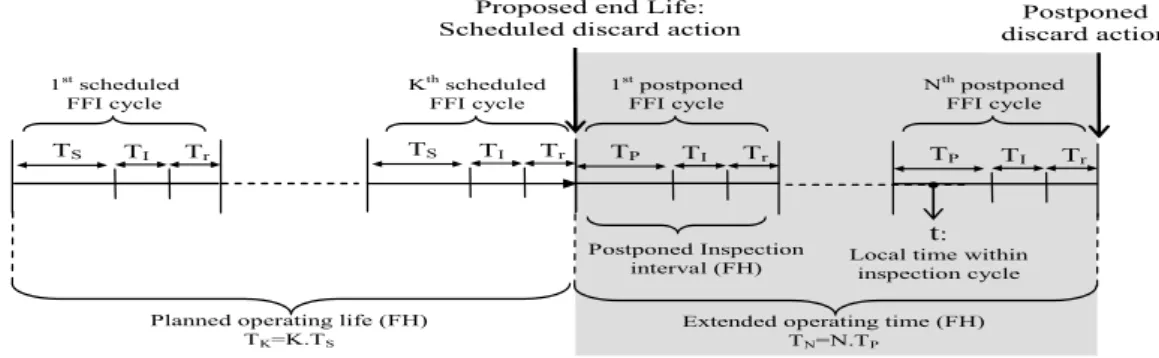
S denotes the original scheduled FFI interval. Schematic description of FFI during planned and extended operating times
Fig. 1 shows a schematic description of maintenance events during the planned and extended operating times. During the initial planned operating life, the system must be grounded to perform an inspection task each time an accumulated number of operating flight hours (hrs) “TS” has been reached. The first inspection is performed after “T” flight hours,
and consequently the Kth inspection will be performed after “T
K” operating flight hours. The inspection task takes TI
hours and, in the case of a finding which leads to a repair, the repair takes Tr hours. Hence, an inspection cycle includes
T, TI and Tr. An expected operating flight time, “TK”, is considered as the unit’s planned operating life, and is divided
into K inspection cycles with the inspection interval TS, so that TK=K.TS .
β β N(t) 1 exp (α 1)T ( α1)T t F TK N P TK N P
will exceed the allowable risk limit, the item should be restored to its original condition. In this situation, when the operator wants to have an extension time, TN, added to the planned operating life (i.e. age, TK) the conditional
probability of failure at time “t” after TK and within the Nth inspection cycle of the extended operating time, is given by:
(7) where, under the postponement strategy, “t” denotes the local time within the Nth inspection cycle, and T
P denotes the
FFI interval; both under postponement strategy.
Unavailability of hidden function
The unavailability of hidden functions is usually measured by the mean fraction of time during which the unit is not operational as protection, i.e. the Mean Fractional Dead Time (MFDT) [2]. If dormant failures occur while the system is in a non-operating state, the system availability can be influenced by the frequency at which the system is inspected. Note that inspection, cannot improve the reliability, but can only improve the function availability [5]. According to Ebeling [5], Rausand and Vatn [9] and Vaurio [13], the function unavailability at time “t” within the Nth inspection
cycle is equal to the conditional probability function, i.e. FN(t). Consequently, the mean interval unavailability within
the Nth inspection cycle, with FFI at every “T” hrs, is given by: dt α t 1)T -(N α 1)T -(N exp 1 T 1 MFDT T 0 β β N) (T,
(8)Fig. 2 illustrates an example of the MFDT of a typical hidden function in an operating period of 10,000 flight hours (FH), for different values of inspection intervals, with α=10000 and β=3. As isshown, when there is an aging effect the MFDT increases in subsequent inspection cycles.
Cost function for postponed FFI
The analytical model presented in this paper is based on the following assumptions:
1) The inspection and repair times associated with findings through FFI, i.e. Ti and Tr (constant values), do not
change with operating time.
TS TI Tr TS TI Tr 1st scheduled FFI cycle Kth scheduled FFI cycle TP TI Tr
Extended operating time (FH) TN=N.TP Nth postponed FFI cycle Postponed discard action TP TI Tr Postponed Inspection interval (FH) 1st postponed FFI cycle
Proposed end Life: Scheduled discard action
t:
Local time within inspection cycle
Planned operating life (FH) TK=K.TS
Figure 1: Schematic description of inspection cycles
Variation of MFDT by operating time
0 0.02 0.04 0.06 0.08 0.1 0.12 0 1000 2000 3000 4000 5000 6000 7000 8000 9000 10000 Operating time (FH) MFD T T=100 T=200 T=300 T=400 T=500 T=600 T=700 T=800 T=900
Figure 2: Variation of MFDT with inspection intervals over time, for different values of FFIintervals, α=10000 and β=3.
4) The failures are completely detectable by inspection/testing.
5) The inspection does not create failure by the nature of the tasks involved. In addition, the maintenance crew do not create failure by their own actions.
6) The failures associated with normal operation of the system are considered in the unavailability and cost model. Common-cause failures originating in design and manufacturing or caused during a demand challenge (an initiating event), are not considered.
7) Postponement of a restoration task does not increase the restoration costs.
8) The costs associated with discard actions are not considered. However, they can be added to the proposed methodology simply.
The following cost parameters are considered for cost modelling of FFI in the postponement scenario:
Direct cost of inspection task, Ci. This is considered as a deterministic value and as a constant in consecutive
inspection cycles.
Cost of possible repair due to a finding, Cr. As the system is undergoing aging, the probability of failure will
change in consecutive inspection cycles. Hence, the expected repair cost within the Nth postponed inspection cycle
can be estimated as: Cr . FN (TP).
Cost of an accident, due to multiple failures, CA. The expected value of CA in the Nth inspection cycle depends on
the expected time during which the function is not available between two postponed inspections, “MFDT(T,N).T”,
and the demand rate for the unit, φ, i.e. “CA . φ .MFDT(TP,N) .T”. For the “safety effect” category, CA refers to the
cost of accidents, e.g. the possible loss of the equipment and/or its occupants. For the “non-safety effect” category, CA may entail possible economic consequences due to the undesired events caused by a multiple failure (e.g.
operational interruption or delays, a higher maintenance cost, and secondary damage to the equipment.
Opportunity cost of the system’s lost production, Coc. This cost is associated with the total system downtime due to
inspection and repair, i.e. Ti and Tr. The expected value can be estimated as: CA .[TI+Tr.FN(T)]
Summing up, the total cost for a series of “N” inspection cycles under the FFI postponement strategy can be estimated by:
Rep 1 ) , P (T , C C.F(T ) C .T T.F(T ) C . .MFDT .T C C N i P i A P i r I oc P i r I N T
(9)and the cost rate function for the extended period of time can be estimated by:
N N T T N C T CRF( ,) (, ) (10) In fact, the CRF is just the additional cost per unit of time for the extended operating life.
Optimum interval
In fact, the operating time TN is divided into N inspections with the interval TP, so that TN=N.TP. The following
equations are valid under certain conditions for FN(T), as proved by Vaurio [13]: ) ( ) ( 0 K K i i T H T F
(11) 2 ) ( ) ( 0 ) , ( 0 K K i K T K i i T MFDT H T F
(12)Fi(T) represents the conditional probability of having just one failure in the ith inspection interval, provided that the
component found functional at (i-1)th inspection. H(T
K) represents the mean number of failures over an interval of
(0,TK). Hence, it is evident that H(TN) overestimates ΣFi(T). However, this overestimation can be acceptable if it is
rational. This estimation depends on the value of α and β. For larger α, and smaller β values, the H(TK) and FN(T)
become more close, and tend to lead to more accuracy in the estimation, while smaller α and larger β values tend to lead to more deviation in the estimation. Moreover, selecting larger T values increases the inaccuracy in the estimation.
Similarly, we can express the mean number of failures within the extended operation time TP as follow: ) ( ) ( ) ( 0 P P K N j i T H T T HT F
(13)
2 ) ( ) ( ) ( 0 ) , ( 0 P P K N i K T N i i T H T T H MFDT T F
(14) Likewise, using the method introduced by Vaurio [13], by substituting (13) and (14) into (9), and denoting TP.N as TN,the following CRF can be derived as a function of the inspection interval T, and the operating time TP:
(15) The optimum inspection interval, TOP, that can minimize the CRF, by a fixed operating time, TN (Hrs), can be
found through this derivative [CRF(T,N)/dTP]=0:
N p N K N K P A N K N K r oc P I oc N K N K r P I T,N T C T ) H(T ) T H(T . T . . C T ) H(T ) T H(T . .T C T .T C T ) H(T ) T H(T C T C CRF Re 2 (16)
However, in case of the “safety effect” category of failure, the postponement process requires adequate proof of risk reduction which satisfies the risk limits. Since such a postponement may increase the cost rate and affect economy negatively, another trade-off analysis is needed to evaluate whether the postponement idea is economical and is acceptable or not.
In the case of the “safety effect” category of failure, the limit conditions for the risk of multiple failures may be dictated through the policies authorities or the companies themselves. Considering Rmax as the maximum permissible
risk limit for the probability of multiple failures, then the postponement process needs to limit the risk of failure under the following supplementary constraint:
max
) , ( max ) , ( R R .MFDTTN MFDTTN (17)Considering a specific FFI interval (e.g. T=200FH), one needs to verify that the value of TOP, obtained from Eq.16,
satisfies Eq. 17, for the values of α, β, φ and Rmax. for the operating time TN. Conclusions
In order to reduce or eliminate the consequences of multiple failures, a specific level of availability of the hidden function is needed. As a common practice, the probability of a multiple failure can be reduced by reducing the unavailability of the hidden function by performing a Failure Finding Inspection (FFI) task, as suggested by RCM methodology. As a common practice, when the component is aging, a replacement task is used after a series of Failure Finding Inspections (FFI) to reduce the risk of multiple failures.
In this study, a cost function (CF) has been developed to identify the cost per unit of time associated with different FFI intervals, for the proposed extended period of life. Moreover, a mathematical model has been defined to obtain the optimal FFI interval, during the extended period of the replacement life. Following this methodology, a lower cost per unit of time is obtained, even if the system is under aging. This approach makes it possible to recognize the real effect of postponement on the total maintenance cost and to evaluate whether performing postponement provides benefits. Following proposed methodology enhance one’s capability to take correct and effective decisions on the postponement of discard tasks. As further research opportunity, it is suggested to develop an integrated model in which both risk and cost are considered in mathematical model.
References
[1]- F.S. Nowlan and H.F. Heap, Reliability Centered Maintenance. San Francisco: United Airlines, 1978. [2]- M. Rausand and A. Høyland, System Reliability Theory: Models, Statistical Methods and Applications.
Hoboken, New Jersey: John Wiley, 2004.
[3]- SAE-JA1012 (2002), A Guide to the Reliability-Centered Maintenance (RCM) Standard, Warrendale, Pa.: Society of Automotive Engineers.
[4]- IEC (1999), 60300 (3-11): Application Guide – Reliability Centred Maintenance, Geneva: International Electrotechnical Commission.
[5]- C.E. Ebeling, An Introduction to Reliability and Maintainability Engineering. New York: McGraw Hill, 1997. [6]- A. Ahmadi, Aircraft Scheduled Maintenance Program Development: Decision Support Methodologies and
Tools. Doctoral thesis, Luleå: Luleå University of Technology, 2010.
[7]- A. Ahmadi and U. Kumar, “Cost based risk analysis to identify inspection and restoration intervals of hidden failures subject to aging,” IEEE Transaction on Reliability, Vol. 60, No.1, 2011, pp 197-209.
[8]- T. Aven and E. Abrahamsen, “On the use of cost-benefit analysis in ALARP processes,” International Journal of Performability Engineering, Vol. 3, No. 3, 2007, pp. 345-353.
[9]- M. Rausand and J. Vatn, “Reliability modelling of surface controlled subsurface safety valves,” Reliability Engineering and System Safety, Vol. 61, No. 1-2, 1998, pp 159-166.
[10]- M. Modarres, Risk Analysis in Engineering: Techniques, Tools, and Trend. Boca Raton,Fla, London: Taylor & Francis, 2006.
[11]- B. Klefsjö and U. Kumar, “Goodness-of-fit tests for the power-law process based on the TTT-plot,” IEEE Trans. on Reliability, Vol. 41, No.4, 1992, pp. 593-598.
[12]- H. Ascher and H. Feingold, Repairable Systems Reliability: Modeling, Inference, Misconceptions and their Causes. New York: Marcel Dekker, 1984.
[13]- J.K. Vaurio, “On time dependent availability and maintenance optimization of standby units under various