Design of a multi-camera system for object identification, localisation, and visual servoing

(1)

School of Innovation, Design and Engineering

V¨

aster˚

as, Sweden

Thesis for the degree of Master of Science in Engineering - Robotics,

30.0 credits

DESIGN OF A MULTI-CAMERA

SYSTEM FOR OBJECT

IDENTIFICATION,

LOCALISATION, AND VISUAL

SERVOING

Ulrik ˚

Akesson

uan13001@student.mdh.se

Examiner: Mikael Ekstr¨

om

M¨alardalen University, V¨aster˚as, Sweden

Supervisor: Fredrik Ekstrand

M¨alardalen University, V¨aster˚as, Sweden

Company supervisor: Per-Lage G¨

otvall,

Volvo GTO, Gothenburg, Sweden June 14, 2019

(2)

Abstract

In this thesis, the development of a stereo camera system for an intelligent tool is presented. The task of the system is to identify and localise objects so that the tool can guide a robot. Different approaches to object detection have been implemented and evaluated and the systems ability to localise objects has been tested. The results show that the system can achieve a localisation accuracy below 5 mm.

(3)

Acknowledgements

I would like to thank the following persons; my supervisors Fredrik Ekstrand and Per-Lage Götvall for guiding me through this thesis work; Erik Hellström at Robotdalen for allowing me to use their robot for recording the test data; Henrik Falk at Mälardalen University for providing the photograph of the test setup (Figure10).

(4)

Abbreviations

BGR Blue, Green, and Red. 16

BRIEF Binary Robust Independent Elementary Features. 7

CAD Computer Aided Design. 12,13

CU130 See3CAM CU130. 12

CU55 See3CAM CU55. 12

CV Computer Vision. 7

EIH Eye-In-Hand. 6–8,10

ETH Eye-To-Hand. 6,7

FOV Field Of View. 7,12

FPS Frames Per Second. 22,25

HBVS Hybrid Based Visual Servoing. 7

HCT Hough Circle Transform. 14,15,17,24,33

HLS Hue, Lightness, and Saturation. 14,16

HSV Hue, Saturation, and Value. 8

I/O Input/Output. 9

IBVS Image Based Visual Servoing. 6,7

ORB Oriented FAST and Rotated BRIEF. 7,15,18,24,33

PBVS Pose Based Visual Servoing. 6

PID Proportional-Integral-Derivative. 8

SIFT Scale-Invariant Feature Transform. 7,15

SURF Speed-Up Robust Feature. 8,15

TaraXL See3CAM TaraXL. 12

(5)

1 Introduction

Ever since industrial robots were first introduced in 1961 [1], one of the main ways for them to interact with the world is through its tool, with which the robot can manipulate objects. In the classic setup which comes to mind, one might think about industrial robots on an assembly line picking up objects, mounting, welding, and doing other specific tasks really well and quite fast. However, the demands from the industry have changed and having a robot that is able to assist in more dynamic tasks in less structured environments is desirable. To have robots transition into dynamic and unstructured environments where it will have to interact with objects which may appear in different locations each time, new approaches need to be implemented. One possible approach is to create an intelligent tool [2], capable of sensing, planning, and instructing the robot in how it should act to reach the goal and complete its task. In this thesis, a vision system for an intelligent tool is developed. The system utilises stereo vision to identify and localise oil filters. This thesis is a part of a bigger project in which Volvo GTO is developing an intelligent tool. The rest of this thesis is structured as follows: In section 2 the background and related works are presented. In section 3 the problem formulation, limitations, hypothesis, and research questions are stated. In section 4 the method and process of evaluation are presented. In sections 6 to 5 the implementation of the different parts of the system are described. In section 8 the test setups are presented. In section 9 the results of the tests are presented. In section 10 the results are discussed and future work presented. In section 11 the conclusion is presented.

(7)

2 Background

Development of intelligent tools that would allow robots to do more generic tasks has been going on for over 40 years. In 1986 Fukuda et al. [3] developed a gripper which could grip both a rubber ball and an aluminium rod securely without oscillating, which was a problem among more conventional grippers when switching between objects of different hardness. In 1998 Tlale et al. [4] developed an intelligent gripper which could sense if the electronic component was properly grasped and in the correct orientation and if either of those conditions was not met it could correct that. In 2018 Pettersson-Gull and Johansson [2] developed an intelligent gripper which was able to pick up and securely grasp a wide variety of household items without any previous knowledge of the items. The gripper could sense when an item approached and adapt its grip for optimal grasp. Common for these grippers are that they could be used for grasping different kinds of objects, and adapting its grip autonomously. However, they do not possess the ability to find the target in the environment and requires the robot to guide them close enough to the target for the intelligence in the tool to grasp the object.

2.1 Visual servoing

One common approach to guide robots towards dynamic targets is to use cameras and visual servoing. In the literature [5,6] visual servoing is described as the task of controlling the motion of a robot with computer vision data acquired through cameras. The goal for all vision-based control strategies is to minimize the error e(t) between the current image data s and the desired image data s∗. The data in s depends on which features that are of interest and varies with the approach.

The two classic approaches of visual servoing are Image Based Visual Servoing (IBVS) and Pose Based Visual Servoing (PBVS), whose principles were proposed by Weiss et al. in 1987 [7]. According to Corke [5], in a PBVS system, s is described by the pose of the target in relation to the camera, which needs to be estimated from the images. Since PBVS strives to match the current pose of the target with the desired pose, geometric data of the target is required. IBVS systems differ from the PBVS system by using features found directly in the image to describe s rather than estimating a pose. Thus eliminating the need for a geometric model of the target.

According to Malis [8], the main advantage of the PBVS approach is that it directly controls the trajectory in Cartesian space which often results in straight paths as demon-strated by Chaumette et al. [6]. However, Malis [8] further states that there is a risk of the image features used for pose estimation leaving the image, which causes PBVS to fail. Since IBVS tracks the features in the image, there is no risk that they leave the image. IBVS is also known to be robust to calibration errors. A drawback with IBVS is that it can produce trajectories which are out of reach for the robot so that, in certain cases, the created trajectory retreats away from the target, a behaviour explained geometrically by Corke and Hutchinsson [9].

2.2 Camera configuration

When adding a camera to the robot or the workspace, there are two commonly mentioned ways to do it, one is attaching the camera to the robot so that it moves with the end effector, and the other is to attach the camera so that it is observing the robot end effec-tor and the workspace. These configurations are referred to as Eye-In-Hand (EIH) and Eye-To-Hand (ETH) respectively by Siciliano et al. [10] or as end-point closed-loop and

(8)

end-point open-loop by Corke [5].

Advantages with the ETH configuration are that the camera Field Of View (FOV) are constant which according to Siciliano et al. [10] means that the accuracy of image mea-surement is virtually constant. Since the camera is fixed in the world there is a risk that the robot moves in such a way that the cameras view of the workspace becomes occluded, this is not a problem with the EIH configuration since it is always moving with the robot. A drawback with the EIH configuration is that since the camera moves with the robot the FOV changes during movement, resulting in variable accuracy. However, when the camera is close to the object, accuracy becomes virtually constant and is generally higher than for ETH.

2.3 Image features

One of the most influential feature detectors in Computer Vision (CV) is the Scale-Invariant Feature Transform (SIFT) keypoint detector [11], stated in both the works of Rublee et al. and Miksik and Mikolajczyk [12,13]. SIFT has been widely used in multiple areas in CV, including object recognition. However, one problem with SIFT is that it is computationally heavy and not suitable for time-constrained applications. Several algo-rithms have been proposed to improve upon SIFT, and in a comparison by Miksik and Mikolajczyk [13] in 2012, they concluded that binary descriptors; such as Binary Robust Independent Elementary Features (BRIEF) [14] and Oriented FAST and Rotated BRIEF (ORB) [12]; provided a good combination of high accuracy and low computational cost making them suitable for time-constrained applications.

2.4 Related work

Kim et al. [15] (2009) utilise an EIH system with stereo vision to guide a robot arm to pick up randomly placed objects. The implementation splits the problem into a gross and fine control strategy based on the end effectors distance to the object.

The gross control strategy utilises SIFT descriptors to detect local features for a rough estimation of the 3D position for the object. The end effector is then driven towards the estimated position. When the end effector is within the proximity threshold the control strategy is changed into a Hybrid Based Visual Servoing (HBVS) scheme which utilises template matching and the extrinsic stereo camera parameters.

A version of IBVS was implemented by Han et al. [16] (2011). Their approach to iden-tifying features is based on the fact that their environment consists of a limited number of colours with high relative contrast. In their work, they use a multi-view setup with monocular cameras. The first camera, which is configured as ETH, finds the target in the environment by using the pinhole camera model to estimate its distance. The other camera is configured as EIH which is used to confirm that the robot is about to grip the object. They show that their implementation successfully can navigate to and pick up a randomly placed object. Due to the use of the pinhole camera model it is required that they manage to detect the entire height of the object to get an accurate depth estimation. Another work utilising a similar colour based approach was conducted by Karuppiah et al. [17] (2018). In the work two monocular cameras configured as ETH and EIH respec-tively is used to identify an object of interest and guide a robot arm to it so that the object can be picked up. In their implementation, the ETH camera is used to estimate a coarse location of the object and the EIH camera is then used to guide the tool to the

(9)

object. Even though successful in grabbing the object and tracking it in the plane, it is never presented how they estimate the distance to the object.

Shaw and Cheng [18] (2016) created an EIH system that identifies an object and calculates its pose. For identification, they utilise the Speed-Up Robust Feature (SURF) algorithm (developed by Bay et al. [19]) and a back projection model for colour matching based on hue and saturation. In the work they use stereo triangulation to retrieve the targets pose. Sayed and Alboul [20] (2014) developed a system that allowed a mobile robot to track and follow an object of interest. To identify the target, colour recognition is used in the Hue, Saturation, and Value (HSV) colour space. The target’s location and size is then used as input to two Proportional-Integral-Derivative (PID) controllers which regulate the steering and distance respectively.

(10)

3 Problem formulation

When a robot’s environment becomes unstructured, previously simple tasks like picking up and manipulating objects becomes harder, for example, if the object is not always located in the same spot. Previously this has been solved by adding vision data to the robot controller by either attaching cameras on the robot or by fixing them in the workspace. A problem with this approach is that it adds work to the robot controller and specialises the robot and the workspace even more. In this thesis, the aim has been to create a multi-camera system for an intelligent tool so that it can detect, localise, and create a path towards an oil filter. Such a system would make it possible to move the intelligence from the robot controller to the tool, distributing the workload of controlling the robot and of observing the environment. For the intended application, the desired accuracy of the localisation is less than 5 mm at a distance of 300 mm as defined by Volvo, and it would be desirable to achieve real-time performance so that data from the cameras can be used continuously. The oil filter used as a target can be seen in Figure 1.

(a) Profile view of the oil filter.

(b) View from ideal starting position.

Figure 1: The oil filter used as a target in this thesis. In 1a the profile of the filter is seen. In 1b the filter is observed from an ideal start position.

3.1 Limitations

The scope of this thesis only includes designing and implementing the vision system for the intelligent tool. Construction of the tool, how the tool should physically interface with the robot, and power and cooling solutions for the tool is not considered in this thesis. Other limiting factors for this thesis are:

The hardware platform for the tool was chosen to be an Nvidia Jetson TX2 (TX2) [21] with a Connect Tech Inc. Orbitty Carrier expansion board [22] as an Input/Output (I/O) interface. The same hardware is used in this thesis.

To allow for faster implementation and testing of different algorithms OpenCV [23] has been used. OpenCV is an open source computer vision library that contains implementations of a wide variety of different algorithms.

During the time frame of this thesis there has been limited access to a robot, thus implementing and evaluating guidance on an actual robot was not possible.

(11)

When access to a robot was given at Robotdalen for the purpose of recording data the maximum velocity that the robot was allowed to be driven with was 0.2 m/s for safety reasons.

A major assumption for this thesis is that the tool will start above the area where the object may exist and that the optical plane of the camera is close to parallel to the workspace.

3.2 Hypothesis

Based on the results in related works, especially those of Kim et al., Han et al., and Karuppiah et al. [15–17], the problem formulation, and the limitations of the thesis the following is hypothesised:

By implementing a binocular EIH vision system on a TX2, it is possible to achieve high accuracy when identifying, localising, and guiding a robot towards an oil filter in real time.

3.3 Research questions

The research questions that is investigated in this thesis are: RQ1: Which image feature(s) can be used to detect an oil filter?

RQ2: What are the constraints necessary to meet the requirements in terms of accuracy and speed for guiding a robot towards an oil filter?

(12)

4 Method

In this thesis, an iterative engineering methodology based on the one described by Tayal is utilised [24]. In short that means that in order to solve the task, possible solutions are researched, implemented, and tested. Depending on the results from the test, the solution is either deemed suitable or a new solution is researched. An illustration of this can be seen in Figure 2.

Figure 2: Illustration of the iterative engineering process.

In this thesis a literature study is performed to research which features can be used for object detection and different detection methods is evaluated. The work is divided into the detection of the target, and the localisation of the target; which can be developed and tested individually. For each part, possible solutions will be investigated through literature and through experiments.

4.1 Evaluation

In order to choose the appropriate solution for this thesis, the different modules need to be evaluated. In the case of detection that involves testing the different algorithms on images captured in different conditions and evaluating based on the detection rate and on the execution time on the TX2. To evaluate the performance of the localisation the cameras were attached to an industrial robot, that moves the camera in the environment while tracking the target. The path obtained from the calculated positions of the target was then compared against the recorded path of the robot and evaluated based on how well the paths align.

(13)

5 Stereo camera rig

In this section, the choice of cameras and the mounting system for the camera is described. 5.1 Camera selection

The different considerations when it came to selecting cameras were availability, depth range, frame rate, resolution, size, colour, and cost. Based on those criteria different cameras where considered, three of which where the See3CAM CU55 (CU55) [25], the See3CAM CU130 (CU130) [26] and the See3CAM TaraXL (TaraXL) [27], all of which were readily available from e-con systems.

Table 1: A comparison between different camera specifications. All the specifications has been taken from their respective datasheets [25–27] and product pages [28–30].

Camera comparison

Camera CU55 CU130 TaraXL

Depth range Not specified Not specified 500 - 3000 [mm] Resolution VGA (640 x 480) FHD (1920 x 1080) 5MP (2592 x 1944) VGA (640 x 480) FHD (1920 x 1080) 13MP (4224x3156) QVGA (2*320) x 240 VGA (2*640) x 480 WVGA (2*752) x 480 Frame rate 60 fps & 30 fps 60 fps, 30 fps & 15 fps 24 fps & 12 fps 60 fps & 30 fps 30 fps &15 fps 5 fps and 2.5 fps 60 fps 60 fps & 30 fps 60 fps & 30 fps

Colour Colour Colour Monochrome

Size [mm] 30 x 30 x 31.3 30 x 30 x 31.3 95 x 17 x 27

Price/unit US$189 US$279 US$349

Given the camera specifications in Table 1, the CU55 is chosen; the colour sensor and the high frame rate for the given resolution being the primary factors making it more suitable than the others. The diagonal FOV (with the included lens) of 135 degrees increase the possibility of finding the object in both images at closer range. Using two individual cameras instead of a dedicated stereo camera also allows for greater flexibility when it comes to mounting the cameras in the tool. It does also allow for the baseline between the sensors to be adapted to the depth range needed.

5.2 Mounting system

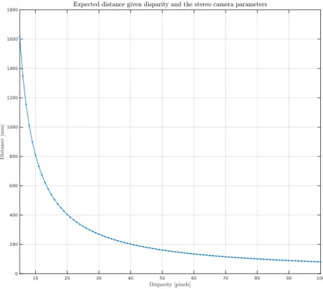
To mount the cameras for testing, a custom bracket was designed in Fusion 360 [31] and 3D printed using an Ultimaker 2+ [32]. The bracket was designed to allow flush and secure mounting of the cameras and to be attached to an RSP TA20-4 tool attachment [33] so that it could be easily mounted to a robot. The Computer Aided Design (CAD) model of the bracket and the TA20-4 is presented in Figure 3. With this design of the bracket, the cameras theoretical depth range lies between 100 mm and 1600 mm as observed in Figure 4. This depth range is suitable given the desired distance of 300 mm mentioned in the problem formulation. The depth range is calculated by eq. 1 where Z is the depth, f is the focal length, T is the baseline between the sensors, and the d is the disparity between the pixels.

(14)

Figure 3: The CAD model of camera bracket for the cameras. The green parts symbolises the cameras, the blue part is the bracket, and the brass part is the tool attachment.

Z = f

dT (1)

(15)

6 Detection

To detect the oil filter three different methods are evaluated, one is to detect areas of interest based on colour, the other to detect circles based on edges, and the third is to detect features using ORB.

6.1 Colour based detection

Since thresholding based on colour worked well in the works by Karuppiah et al., Kim et al., and Han et al. [15–17], and since the object of interest has a distinct shape and colour, a similar approach for detecting the object is evaluated in this thesis. The first step of this approach is to convert the image to the Hue, Lightness, and Saturation (HLS) colour space. The reasoning behind this is that in HLS the hue, lightness and saturation are separated in a way that mimics human perception of colour as stated by Ibraheem et al. [34]. They also state that it is an appropriate colour space for image segmentation. The second step involves creating a binary mask, in which the only regions remaining are the ones that contain the colour of the object. The binary mask is then used in the findContours algorithm [35] which finds all the points making up contours in the image. The area and centroid of the contour are then calculated using the image moments as described by Rocha et al. [36] where the area is used to filter out objects that are too large or too small to be the object. Finally, based on the knowledge that the shape of the object will be circular, a circularity test as the one proposed by Mingqiang et al. [37] is applied to remove false detections. In Figure 5 the effects on the image of the different steps in the process can be seen.

6.2 Edge based detection

Since the shape of the oil filter when observed from above is fairly circular, as seen in Figure 6a, using a method that finds circles to detect the oil filter seems feasible. One popular algorithm for finding circles is the Hough Circle Transform (HCT) [38]. It has been implemented in a multitude of different applications where circular objects were to be detected, such as heads in the work by Liu et al. [39], or eyes as in the work by Hu et al. [40], or other generic circular objects as in the work by Ni et al. [41]. Liu et al. [39] describes the strengths of HCT as that it is robust to unclear object boundaries due to overlapping objects or distortion from noise or ambient light.

For this evaluation the HCT algorithm is implemented as described in [42]. The different steps used when implementing HCT are presented in Figure 6 and includes converting the image to greyscale and blurring it, those steps are a prerequisite for the edge detector which creates the binary edge image that the circles are detected in. Similarly to the previous method the area of the found circles will be used to remove any objects that are too small or too large. A drawback of HCT in the context of this thesis is that since it only works on binary images the colour information is not utilised when searching for possible targets.

(16)

6.3 Feature based detection

The feature detector and descriptor that the previously mentioned methods are compared to is ORB [43]. ORB was developed by Rublee et al. [12] as a faster alternative to SIFT and SURF [11,19]. In their tests they could show that ORB is as accurate as the other methods while having a much lower computational cost, making it suitable for time-constrained applications or weaker hardware, something that is corroborated by Miksik and Mikolajczyk, and Tareen and Saleem [13,44] in their comparative analysis of different feature detectors and descriptors available in OpenCV. To evaluate this method it is implemented as described in the book by Kaehler et al. [45]. The default parameters for ORB is used, and a template image of the object is used to match against the test images. As can be seen in Figure 7 the image is first converted to greyscale and blurred (as in the case of HCT), then the ORB features and descriptors are detected and matched, and the 10% of matches with the best matching score is used for detecting the object.

(17)

(a) Start image (b) Image convereted to HLS (imshow prints images as if they were represented in the Blue, Green, and Red (BGR) colour space).

(c) Create mask (d) Find contours

(e) Detection results

(18)

(a) Start image (b) Image convereted to grayscale

(c) Blur image (d) Find edges (note that this step is done within the HCT algorithm and this image only used as visualisation).

(e) Find circles (f ) Detection results

(19)

(a) Start image (b) Convert the image to greyscale.

(c) Blur the image. (d) Find and match features and descriptors. Valid matches are connected with lines.

(e) Detection results

(20)

7 Localisation

After the object has been detected it needs to be localised in the world so that a robot could move the tool to its position. In order to find the world coordinate of the object, stereo triangulation is utilised. In order to triangulate, the object needs to be found in both images. Since the cameras are calibrated and the images rectified to fulfil the epipolar constraint, it can be assumed that the object can be found on the same horizontal line in both images as described by Brown et al. [46]. In this case, that means utilising the template matching algorithm in OpenCV [47] with the detected object and a small region around it as a template. The algorithm has been optimised based on the epipolar constraint so that only a small part of the image corresponding to the same rows as the template needs to be searched. After finding the coordinates of the centroid of the object in both images, the world coordinate of the detected object is calculated using the triangulatePoints [48] function which returns the homogenous world coordinates of a stereo pair.

7.1 Rejection of false objects

To reduce the risk of tracking a false match a simple rejection algorithm is implemented. The algorithm compares the area returned by the detection algorithm Aiwith the expected

area of the object Ae and if the difference between them is greater than a threshold the

detection is rejected. The expected area is calculated by the similar triangles relation from the pinhole camera model seen in eq. 2 where hi is the height of the object in the image,

hw is the known height of the object in the world, f is the focal length of the camera,

and Z is the depth to the object. However, instead of only considering the height it is adapted to calculate the area as seen in eq. 3 where Aw is the known area of the object

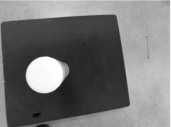
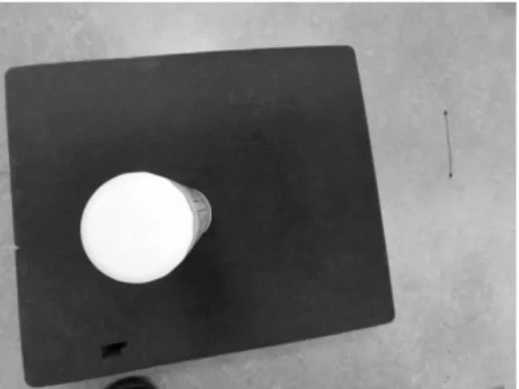
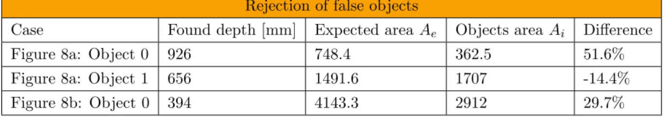
in the world. In Figure 8 cases with and without false objects can be seen; in Table 2 the data and the output of the algorithm is presented.

hi = f Zhw (2) Ae= f2 Z2Aw (3)

Table 2: The data used by the rejection algorithm on the cases presented in Figure 8.

Rejection of false objects

Case Found depth [mm] Expected area Ae Objects area Ai Difference

Figure 8a: Object 0 926 748.4 362.5 51.6%

Figure 8a: Object 1 656 1491.6 1707 -14.4%

(21)

(a) Image where 2 objects are detected. As can be seen in Table 2 the error for detection 1 is smaller than that of the false detection.

(b) Image where only one true detection has been made. As can be seen in Table 2 the error is slightly below 30% which has been chosen as the threshold for rejection.

Figure 8: Examples of the rejection algorithm. Note that for the case in Figure 8a most of the filtration parameters for the colour based detection had to be modified to allow for more general matches.

(22)

8 Test setup

In order to test the detection and localisation different sets of tests were designed. 8.1 Detection

To evaluate which of the three approaches are the most suitable for the application a set of 51 images of the oil filter has been collected in different lighting with different distance and orientation of the object and where the centroid point and the minimum bounding rectangle of the object have been manually identified. The criteria used for the comparison is the detection ratio and the execution time on the TX2. A detection is considered valid if the centroid of the detected object lies within a 5-pixel radius of the manually detected centroid and the absolute difference between the sides of the manually identified and automatically detected bounding box is less than or equal to 15 pixels. In Figure 9a an example of a valid detection is presented and in figures 9b through 9d examples of false detections can be seen.

(a) Example of a valid detection (b) Example of a false detection

(c) Example of a false detection (d) Example of a false detection

Figure 9: Examples of valid and false detections.

8.2 Localisation

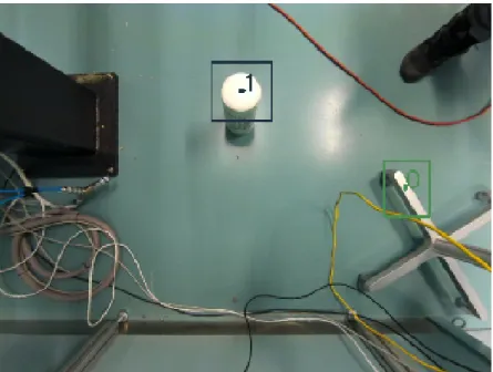
To evaluate how well the system can find the world coordinates of the object the camera was mounted to a robot arm that was programmed to drive a certain path. The path of the robot is recorded using RobotStudio 6.08 [49] with the camera mounted as seen in

(23)

Figure 10. For these tests, the camera’s resolution was set to 640x480 and the frame rate was set to 30 Frames Per Second (FPS). Since the robot and the camera has their own coordinate systems, they are calibrated so that the paths can be correlated. Furthermore, it was not possible to time synchronise the camera and the robot for these tests. The data are synchronised offline by shifting the time so that the movement through the origin happens at the same time for both the recorded and calculated data. This point is chosen since it is repeatable for all the cases. The test set is made up of six unique cases which are each run twice, creating a test set of 12 cases. The entire set can be seen in Table 3. The variables that are controlled in these test cases are the velocity and the path of the object. The attributes that are evaluated are the accuracy of each individual case and precision over all the cases.

Table 3: The test cases for the evaluation of the localisation. The path is a straight line along the axes, with the exception of cases one and two, in which the path is more elaborate. In the single axis cases (3-8) the movement is in intervals of 100 mm with a stop for 3 seconds in between each step.

Localisation test cases

Case no Movement along Velocity [m/s] Type

1 & 2 xyz 0.05 Continuous

3 & 4 x 0.05 Step

5 & 6 y 0.05 Step

7 & 8 z 0.05 Step

9 & 10 xyz 0.2 Continuous

(24)

Figure 10: The physical test setup with the camera with its bracket mounted to a robot. Pho-tograph provided by H. Falk [50].

(25)

9 Results

In this section the results from the detection and localisation tests are presented in sub-sections 9.1 and 9.2 respectively.

9.1 Detection

The results from the detection tests show that the colour based method on average executes in 3.1 ms with a ratio of valid detections of 72.5%. The method based on HCT executes in 5.7 ms on average with a ratio of valid detections of 19.6%. The average execution time of ORB is 9.5 ms with a valid detection ratio of 1.9%. Data of the results from the detection test are presented in Table 4. In that table, it can be seen that 90% of the valid detections from HCT have been found by the other approaches. However, 54.9% of the colour based detections are unique.

Table 4: The results from the comparison between the different detection algorithms. On average the colour based detection is 45.8% faster than HCT and 71.1% faster than ORB on the TX2.

Detection results

Execution time [ms] Detections Method

Min Max Avg. All Valid Unique Colour based 2.5915 4.4884 3.0615 40/51 37/51 28/51 Hough circle transform 4.4646 20.7277 5.6506 11/51 10/51 1/51 ORB 8.3901 15.0458 10.5853 51/51 1/51 0/51

The execution times of the different methods are presented in full in Figure 11 and as previously mentioned it can be seen that the colour based detector is faster than the other methods.

(26)

Figure 11: The execution time for the different detection methods for each of the 51 test images.

9.2 Localisation

In Table 5 the minimum, maximum, and average absolute error for each of the cases when the colour based detection method is used are presented. As can be seen in this table the absolute error over X and Y is generally smaller than the absolute error over Z; in figures 12 to 17 the same behaviour can also be observed. In those figures, it can also be seen that the error gets closer to zero and oscillates less the closer to the origin the camera is. In figures 15, 16, and 17 it can also be observed that when the camera is stationary the precision and accuracy in the measurements increases compared to when the robot is moving. By comparing figures 13 and 14, which corresponds to the same path at velocities of 0.05 m/s and 0.2 m/s respectively it can be seen that the error at further distances is worse at higher velocities.

From Table 6 it can be seen that the average execution time in a majority of the cases is faster than the frame rate of the camera which for these tests were set to 30 FPS. In figures 12 to 17 the loop execution times for each iteration in which the object was detected is presented and it can be observed that in all the cases most of the time the loops are faster than the aforementioned frame rate. It can be observed that in the majority of the cases where the execution time is slower it only takes up to 2 ms longer.

(27)

Table 5: Minimum, maximum, and average absolute error [mm] of the estimated position relative the recorded position. In these tests the colour based detection method was used.

Absolute error Case no 1 2 3 4 5 6 X 0.00 0.00 0.00 0.00 0.00 0.00 Y 0.03 0.01 0.00 0.00 0.01 0.01 Min Z 0.02 0.04 0.66 0.66 0.79 0.79 X 46.58 44.65 70.89 55.58 7.57 6.83 Y 33.15 31.16 8.13 8.14 38.29 44.30 Max Z 78.62 78.65 76.58 76.58 47.72 39.01 X 6.35 6.47 10.74 10.78 4.02 4.10 Y 4.49 4.94 2.90 2.88 5.33 5.74 Avg. Z 17.65 20.14 25.55 26.59 12.25 9.97 Case no 7 8 9 10 11 12 X 0.00 0.05 0.00 0.06 0.01 0.01 Y 0.07 0.08 0.06 0.03 0.01 0.01 Min Z 0.16 0.02 0.14 0.05 0.07 0.11 X 5.49 4.55 30.58 62.16 62.42 55.31 Y 5.60 5.60 19.73 44.68 46.43 43.53 Max Z 95.79 70.43 60.09 71.13 107.98 102.29 X 2.08 2.16 7.80 8.31 10.92 9.44 Y 2.13 2.16 5.28 5.98 5.49 4.25 Avg. Z 11.08 11.56 16.76 16.93 22.04 18.94

Table 6: Minimum, maximum, and average loop execution time [ms] for the different test cases when the colour based detection method was used.

Loop execution time

Case no 1 2 3 4 5 6 Min 26.19 24.37 24.43 24.63 26.60 27.03 Max 47.06 489.18 41.07 40.81 46.15 38.84 Avg. 32.76 33.29 33.69 33.47 32.79 33.43 Case no 7 8 9 10 11 12 Min 25.50 30.22 24.72 23.91 25.21 25.45 Max 425.67 36.12 42.01 41.90 42.13 42.01 Avg. 33.62 33.08 33.01 33.10 32.76 32.92

(28)

(a) The estimated path from tracking the object compared to the recorded path of the robot.

(b) Absolute error of the estimated position relative the recorded position plotted over time.

(c) Loop execution time during case 1. The red line corresponds to the frame rate of the camera

Figure 12: Results for case 1, in which the robot drove continuously along a path through X, Y, and Z at 0.05 m/s and the colour based detection method was used.

(29)

Figure 13: Results for case 9, in which the robot drove continuously along a straight line through X, Y, and Z at 0.2 m/s and the colour based detection method was used.

(30)

Figure 14: Results for case 11, in which the robot drove continuously along a straight line through X, Y, and Z at 0.05 m/s and the colour based detection method was used.

(31)

(a) The estimated position and the recorded position plotted over time.

(b) Error of the estimated position relative the recorded position plotted over time.

Figure 15: Results for case 3, in which the robot drove along the X-axis in steps of 100 mm at 0.05 m/s and the colour based detection method was used.

(32)

(a) The estimated position and the recorded position plotted over time.

Figure 16: Results for case 5, in which the robot drove along the Y-axis in steps of 100 mm at 0.05 m/s and the colour based detection method was used.

(33)

(a) The estimated position and the recorded position plotted over time

Figure 17: Results for case 7, in which the robot drove along the Z-axis in steps of 100 mm at 0.05 m/s and the colour based detection method was used.

(34)

10 Discussion & future work

Possible features that can be used for detection have been investigated in literature and it was found that previous works have had success with utilising features such as colour, shape, and feature detectors. Three methods have been implemented and tested to eval-uate which method and features are appropriate to detect an oil filter. The results from this test show that the colour based detection method is more appropriate for implemen-tation on the TX2 than the HCT and ORB for the specific task in this thesis; not only yielding a higher ratio of valid detection but also having a faster execution time. It can be seen that ORB detected something in every test image, however only one of those was a valid detection. The lack of texture on an oil filter when viewed from above makes it a hard target to find features with unique descriptors on; resulting in the low accuracy of the ORB detector. Although colour based detection is found to be the most suitable of the tested implementations and certainly performs well enough to allow for the local-isation to achieve good results; it still is not able to find the oil filter in every case. It would be interesting to investigate if applying a preprocessing step to the colour based detector, or perhaps if the detector itself can be used as a preprocessing step for another algorithm, would increase the valid detection ratio. An alternative solution to increase the valid detections could be to apply multiple different algorithms which could produce complementary detections.

The results from the localisation tests show that the implemented system is able to track the object fairly well, especially in X and Y where the absolute error most of the time is less than or equal to 10 mm, and while close to the origin or stationary the error was less than or equal to 5 mm; a result which achieves the desired goal in the problem formulation. The error in Z was most of the time larger than the error in X and Y, and it showed more oscillation, with the oscillations being worse the further away from the target the camera is. However, that behaviour may be expected from investigating eq. 1 were it can be seen that small errors in the disparity can result in large errors in depth. This is visualised in Figure 18 where it can be seen how the same error in disparity causes a larger error in distance at further distances.

The fact that the accuracy and precision are greatly increased while the camera is station-ary indicates that a feasible way to guide a robot with the system would be to make short stops every so often to allow for the best possible measurement. By implementing micro stops it might also be possible to achieve good measurements while driving the robot at a higher velocity. Alternatively, implementing some sort of filtering; either by hardware or by software; might decrease the error in the measurements while the camera is in motion if it is found that it is preferable that the robot moves continuously without repeated stops. However, further investigation into both of these ideas are necessary.

In the result section, it could be seen that in some cases the system takes longer to exe-cute than the frame rate of the cameras, an issue with this is the risk that the system will guide the robot based on old location data and thus reduce the accuracy of the servoing. A possible solution to this problem would be to investigate ways to optimise the code. As the TX2 has a stronger GPU than CPU, finding ways to utilise that better could lead to faster execution times. Another solution could be to keep track of the execution time and if it is noticed that the system is not able to keep up, frames could be skipped to make sure that the data used to localise the target is current. However, a drawback with

(35)

Figure 18: Relationship between error in disparity up to three pixels and error in depth.

that approach would be the reduction of resolution since the movement would be larger between two localisations and that the velocity would need to be decreased to retain the resolution.

In the loop execution time data presented in Table 6 it could be seen that in case 2 and 7 the max time went above 400 ms. This is an anomaly in the data that could be caused by a temporary loss of connection to the cameras. However, further investigation into this behaviour is needed to verify the cause. Finally in figures 15, 16, and 17 it can be observed that the timing of the recorded and estimated data do not add up. This is believed to be caused by a combination of the way the frames are read from the camera and that the loop execution time is not always fast enough. A way to test this could be to run the cameras slower but that is unfortunately not possible due to limitations in the hardware not allowing the cameras to be used at a lower frame rate at the resolution used for the tests.

(36)

11 Conclusion

In this thesis, a stereo camera system which is able to detect and localise an oil-filter with an accuracy of less than 5 mm in certain cases has been developed. It has been showed that it is possible to achieve this by using an Nvidia Jetson TX2 and off the shelf cameras. During this thesis, different features and methods of detecting those features have been compared and it has been shown that a combination of colour and shape (as described in section 6.1) are suitable features for detecting an oil filter. Additionally, a strategy to remove false detections has been presented.

The system’s ability to localise and track the object has been tested with both continuous motion in different velocities and when the camera stops along the path. It was seen that while the camera was stationary a more accurate and precise localisation is achieved and thus that movement pattern would be a good strategy to achieve good servoing of a robot.

(37)

References

[1] Robotic Industries Association, “UNIMATE // The First Industrial Robot,” [Online]. Available: https://www.robotics.org/joseph-engelberger/unimate.cfm Last accessed: 2019-02-07.

[2] P. Pettersson-Gull and J. Johansson, “Intelligent robotic gripper with an adaptive grasp technique,” 2018.

[3] T. Fukuda, N. Kitamura, and K. Tanie, “Flexible handling by gripper with considera-tion of characteristics of objects,” in Proceedings. 1986 IEEE Internaconsidera-tional Conference on Robotics and Automation, vol. 3, April 1986, pp. 703–708.

[4] N. S. Tlale, R. Mayor, and G. Bright, “Intelligent gripper using low cost industrial sensors,” in IEEE International Symposium on Industrial Electronics. Proceedings. ISIE’98 (Cat. No.98TH8357), vol. 2, July 1998, pp. 415–419 vol.2.

[5] P. Corke, “Vision-based control,” in Robotics, Vision and Control: Fundamental Algorithms In MATLAB® Second, Completely Revised, Extended And Updated Edition. Cham: Springer International Publishing, 2017, pp. 537–563. [Online]. Available: https://doi.org/10.1007/978-3-319-54413-7 15

[6] F. Chaumette, S. Hutchinson, and P. Corke, “Visual servoing,” in Springer Handbook of Robotics. Cham: Springer International Publishing, 2016, pp. 841–866. [Online]. Available: https://doi.org/10.1007/978-3-319-32552-1 34

[7] L. Weiss, A. Sanderson, and C. Neuman, “Dynamic sensor-based control of robots with visual feedback,” IEEE Journal on Robotics and Automation, vol. 3, no. 5, pp. 404–417, October 1987.

[8] E. Malis, “Survey of vision-based robot control,” ENSIETA European Naval Ship Design Short Course, Brest, France, vol. 41, p. 46, 2002.

[9] P. I. Corke and S. A. Hutchinson, “A new partitioned approach to image-based visual servo control,” IEEE Transactions on Robotics and Automation, vol. 17, no. 4, pp. 507–515, Aug 2001.

[10] B. Siciliano, L. Sciavicco, L. Villani, and G. Oriolo, “Visual servoing,” in Robotics: Modelling, Planning and Control. London: Springer London, 2009, pp. 407–467. [Online]. Available: https://doi.org/10.1007/978-1-84628-642-1 10

[11] D. G. Lowe, “Object recognition from local scale-invariant features,” in Proceedings of the Seventh IEEE International Conference on Computer Vision, vol. 2, Sep. 1999, pp. 1150–1157 vol.2.

[12] E. Rublee, V. Rabaud, K. Konolige, and G. Bradski, “Orb: An efficient alternative to sift or surf,” in 2011 International Conference on Computer Vision, Nov 2011, pp. 2564–2571.

[13] O. Miksik and K. Mikolajczyk, “Evaluation of local detectors and descriptors for fast feature matching,” in Proceedings of the 21st International Conference on Pattern Recognition (ICPR2012), Nov 2012, pp. 2681–2684.

(38)

[14] M. Calonder, V. Lepetit, C. Strecha, and P. Fua, “Brief: Binary robust independent elementary features,” in Computer Vision – ECCV 2010, K. Daniilidis, P. Maragos, and N. Paragios, Eds. Berlin, Heidelberg: Springer Berlin Heidelberg, 2010, pp. 778–792.

[15] D. Kim, R. Lovelett, and A. Behal, “Eye-in-hand stereo visual servoing of an assistive robot arm in unstructured environments,” in 2009 IEEE International Conference on Robotics and Automation, May 2009, pp. 2326–2331.

[16] L. Han, X. Wu, C. Chen, and Y. Ou, “The mobile manipulation system of the house-hold butler robot based on multi-monocular cameras,” in 2011 IEEE International Conference on Information and Automation, June 2011, pp. 726–731.

[17] P. Karuppiah, H. Metalia, and K. George, “Automation of a wheelchair mounted robotic arm using computer vision interface,” in 2018 IEEE International Instru-mentation and Measurement Technology Conference (I2MTC), May 2018, pp. 1–5. [18] J. Shaw and K. Y. Cheng, “Object identification and 3-d position calculation using

eye-in-hand single camera for robot gripper,” in 2016 IEEE International Conference on Industrial Technology (ICIT), March 2016, pp. 1622–1625.

[19] H. Bay, T. Tuytelaars, and L. Van Gool, “Surf: Speeded up robust features,” in Computer Vision – ECCV 2006, A. Leonardis, H. Bischof, and A. Pinz, Eds. Berlin, Heidelberg: Springer Berlin Heidelberg, 2006, pp. 404–417.

[20] L. A. A. Sayed and L. Alboul, “Vision system for robot’s speed and position con-trol,” in 2014 13th International Conference on Control Automation Robotics Vision (ICARCV), Dec 2014, pp. 1010–1014.

[21] NVIDIA Corporation, “NVIDIA Jetson TX2 Module,” [Online]. Available: https: //developer.nvidia.com/embedded/buy/jetson-tx2 Last accessed: 2019-02-07.

[22] Connect Tech Inc., “Orbitty Carrier for NVIDIA® Jetson TX2/TX2i/TX1,” [Online]. Available: http://connecttech.com/product/ orbitty-carrier-for-nvidia-jetson-tx2-tx1/ Last accessed: 2019-02-10.

[23] OpenCV, “OpenCV 3.4.1,” [Online]. Available: https://opencv.org/opencv-3-4/Last accessed: 2019-05-13.

[24] S. Tayal, “Engineering design process,” International Journal of Computer Science and Communication Engineering, vol. 18, no. 2, pp. 1–5, 2013.

[25] e-con Systems India Pvt Ltd, “See3CAM CU55 Datasheet,” https://www. e-consystems.com/5mp-low-noise-usb-camera.asp#documents, 12 2018, revision 1.3.

[26] ——, “See3CAM CU130 Datasheet,” https://www.e-consystems.com/ UltraHD-USB-Camera.asp#required-documents, 9 2017, revision 1.2.

[27] ——, “See3CAM TaraXL Datasheet,” https://www.e-consystems.com/ 3d-usb-stereo-camera-with-nvidia-accelerated-sdk.asp#documents, 2 2019, revi-sion 1.1.

[28] ——, “See3CAM CU55 Key features,” [Online]. Available: https://www. e-consystems.com/5mp-low-noise-usb-camera.asp#key-featuresLast accessed: 2019-02-07.

(39)

[29] ——, “See3CAM CU130 Key features,” [Online]. Available: https://www. e-consystems.com/UltraHD-USB-Camera.asp#4k-usb-camera-features Last ac-cessed: 2019-02-07.

[30] ——, “See3CAM TaraXL Key features,” [Online]. Available: https: //www.e-consystems.com/3d-usb-stereo-camera-with-nvidia-accelerated-sdk.asp# key-features Last accessed: 2019-02-07.

[31] Autodesk, “Fusion 360,” [Online]. Available: https://www.autodesk.com/products/ fusion-360/overview Last accessed: 2019-03-08.

[32] Ultimaker, “Ultimaker 2+,” [Online]. Available: https://ultimaker.com/en/ products/ultimaker-2-plusLast accessed: 2019-03-08.

[33] Robot System Products, “Tool Changer TC4,” [Online]. Available: http://wp303. webbplats.se/docs/products/TC20.pdf Last accessed: 2019-05-07.

[34] N. A. Ibraheem, M. M. Hasan, R. Z. Khan, and P. K. Mishra, “Understanding color models: a review,” ARPN Journal of science and technology, vol. 2, no. 3, pp. 265– 275, 2012.

[35] OpenCV, “findContorus OpenCV 3.4.1,” [Online]. Available:

https://docs.opencv.org/3.4.1/d3/dc0/group imgproc shape.html# ga17ed9f5d79ae97bd4c7cf18403e1689a Last accessed: 2019-05-08.

[36] L. Rocha, L. Velho, and P. C. P. Carvalho, “Image moments-based structuring and tracking of objects,” in Proceedings. XV Brazilian Symposium on Computer Graphics and Image Processing, Oct 2002, pp. 99–105.

[37] Y. Mingqiang, K. Kidiyo, and R. Joseph, “A survey of shape feature extraction techniques,” in Pattern Recognition, P.-Y. Yin, Ed. Rijeka: IntechOpen, 2008, ch. 3. [Online]. Available: https://doi.org/10.5772/6237

[38] OpenCV, “houghCircleDetector CUDA OpenCV 3.4.1,” [Online]. Available:

https://docs.opencv.org/3.4.1/da/d80/classcv 1 1cuda 1 1HoughCirclesDetector. html#details Last accessed: 2019-05-08.

[39] H. Liu and S. Lin, “Detecting persons using hough circle transform in surveillance video.” in VISAPP 2010 - Proceedings of the Fifth International Conference on Com-puter Vision Theory and Applications, Angers, France, May 17-21, 2010 - Volume 2, 01 2010, pp. 267–270.

[40] S. Hu, Z. Fang, J. Tang, H. Xu, and Y. Sun, “Research of driver eye features detection algorithm based on opencv,” in 2010 Second WRI Global Congress on Intelligent Systems, vol. 3, Dec 2010, pp. 348–351.

[41] J. Ni, Z. Khan, S. Wang, K. Wang, and S. K. Haider, “Automatic detection and counting of circular shaped overlapped objects using circular hough transform and contour detection,” in 2016 12th World Congress on Intelligent Control and Automa-tion (WCICA), June 2016, pp. 2902–2906.

[42] OpenCV, “houghCircle OpenCV 3.4.1,” [Online]. Available:

https://docs.opencv.org/3.4.1/dd/d1a/group imgproc feature.html# ga47849c3be0d0406ad3ca45db65a25d2d Last accessed: 2019-05-08.

(40)

[43] ——, “ORB CUDA OpenCV 3.4.1,” [Online]. Available: https://docs.opencv.org/3. 4.1/da/d44/classcv 1 1cuda 1 1ORB.html Last accessed: 2019-05-09.

[44] S. A. K. Tareen and Z. Saleem, “A comparative analysis of sift, surf, kaze, akaze, orb, and brisk,” in 2018 International Conference on Computing, Mathematics and Engineering Technologies – iCoMET 2018, 03 2018.

[45] A. Kaehler and G. Bradski, Learning OpenCV 3: Computer Vision in C++ with the OpenCV Library. O’Reilly Media, 2016. [Online]. Available:

https://books.google.se/books?id=SKy3DQAAQBAJ

[46] M. Z. Brown, D. Burschka, and G. D. Hager, “Advances in computational stereo,” IEEE Transactions on Pattern Analysis & Machine Intelligence, no. 8, pp. 993–1008, 2003.

[47] OpenCV, “Template matching CUDA OpenCV 3.4.1,” [Online]. Available: https:// docs.opencv.org/3.4.1/d2/d58/classcv 1 1cuda 1 1TemplateMatching.html Last ac-cessed: 2019-05-13.

[48] ——, “Triangulate points OpenCV 3.4.1,” [Online]. Available: https://docs.opencv. org/3.4.1/d9/d0c/group calib3d.html#gad3fc9a0c82b08df034234979960b778c Last accessed: 2019-05-13.

[49] ABB, “RobotStudio,” [Online]. Available: https://new.abb.com/products/robotics/ sv/robotstudio/nedladdningsbara-programLast accessed: 2019-03-08.

[50] H. Falk, “Camera mounted to robot,” 2019, [Photograph], (From the collection of M¨alardalen University).