Analysis of infrared heating rates in observed cloud layers

Analysis of Infrared Heating Rates in Observed Cloud Layers

by

Lori Diane Olsen

Department of Atmospheric Science

Colorado State University

ANALYSIS OF INFRARED HEATING RATES IN OBSERVED CLOUD LAYERS

Submitted by

Lori Diane Olsen

Department of Atmospheric Sciences

ABSTRACT

ANAL YSIS OF INFRARED HEATING RATES IN OBSERVED CLOUD LAYERS

A vertical heating rate profile is computed for an observed vertical distribution

or

cloud layers and liquid water content. One case looks at multiple-layered clouds in the western tropical Pacific Ocean and the other case examines a single-layer cloud in the eastern subtropical Atlantic Ocean. A broadband radiative transfer program is used to calculate heating and cooling rates. This method uses the Goody random statistical model to compute transmission through the clear air and cloud and assumes a linear absorption coefficient which is valid for small drops. Observations of the cloud scene are made from visible and infrared satellite imagery. The vertical distribution of clouds is determined from rawinsonde humidity profiles or ground based millimeter wavelength radar. Integrated cloud liquid water is computed from microwave brightness temperatures retrieved from satellite.

When the heating and cooling rates are integrated over 200 mb layers, cooling that results from the flux divergence at cloud top ranges from -0.28 OK/day to -0.63 OK/day. while the warming at the cloud base is less than 0.2 OK/day. This indicates that cloud top cooling due to infrared radiation plays a role in the diabatic heating and cooling of the atmosphere.

The cloud forcing in each case was also investigated. The multiple-layered clouds associated with the tropical convection increased cooling of the atmosphere at the cloud top, but the largest percent change was in the middle layers due to infrared heating. The single-layer cloud in the Atlantic Ocean case was too low to have much heating at the cloud base, but the cooling at cloud top was significant.

ACKNOWLEDGEMENTS

This research was supportedbythe Department of Defense Geosciences, project,

TABLE OF CONTENTS CIIAPTER 1 1 INTRODUCTION CHAPTEH. 2 -t BACKGROUND 2.1 Cloud Analysis 4

2.1.1 Determination of cloud type 5

2.1.2 Distribution of cloud layers 6

2.2 Calculation of heating and cooling rates 10

2.2.1 Radiative transfer theory 10

2.2.2 Radiative transfer with clouds 13

2.2.3 Calculation of transmission 16

2.2.4 Comparison of LWBAND output to CAGEX data 18

) ) ~ S ... f l ' d i dd' 'b . "'0

_._.) . ensltlvlty0 leatmg rate to water content an c ou Istn utlOn ... _

2 ... [ " d.J ,lqUl water retneva usmg passive microwave" I ' . . "'6

"'-2.3.1 Theory 26 2.3.2 Descriptionofmethod 27 CHAP1"ER 3 31 DATA 3.1 Case selection 31 3. I . I Case I 31 3.1.2 Case ll 35

3.2 Satellite data sets 38

3.2.1 SSM/I 38

3.2.2 GMS 39

3.2.3 Meteosat 39

3.2.4 Sea surface data AO

3.3 Satellite data set remapping .40

CHAPTER 4 42

CASE I

4.1 Analysis of clouds in scene .42

4.1.1 Cloud type from satellite VIS and IR imagery .42

4.1.2 Vertical cloud structure over selected sounding sites .42

.4-1-4.2.2 Vertical distribution of liquid water .47

4.3 IIcating and cooling rates 52

4.3.1 Analysis 52

4.3.2 Cloud forcing 60

<:IIAPTER 5 63

CASE [l

5.1 Analysis of clouds 63

5.1.1 Cloud type from satellite visible and IR analyses 63 5.1.2 Vertical cloud structure over sounding site 63

5.2 Liquid water retrieval... 70

5.2.1 Horizontal distribution of liquid water over scene 70 5.2.2 Vertical distribution of liquid water in specified clouds 71

5.3 Heating and cooling rates 76

CIIAP'fER. 6 82

CONCLUSION

LIST OF FIGURES

Figure 2.1: Schematic diagram of a bispectral cloud classification scheme [Kidder and

Vander Haar, 1995] 6

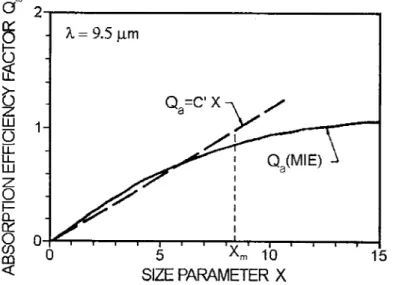
Figure 2.2: Absorption efficiency factor, Qa' as a function of size parameter, x(=2rrr/A.)

[from Pinnick et a1. 1979] 14

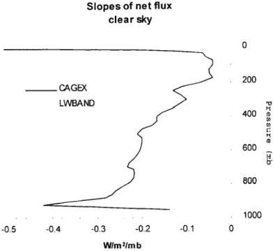
Figure 2.3: Comparison of CAGEX and LWBAND net flux slope in clear sky 19 Figure 2.4: Comparison of CAGEXand LWBAND net flux slopes with a cloud layer

present. 19

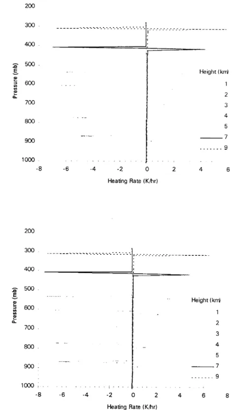
Figure 2.5: Change in heating rates with height for a 300 meter thick cloud with aLWC

of 0.2 g/mJ(Case I)and 0.6 g/m3Case II) 22

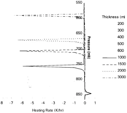
Figure 2.6: Heating and cooling rates when the thickness of the cloud is changed. Cloud base is held fixed at850 mb and LWC

=

0.2 g/m3 23 Figure 2.7: Heating rates for a range ofLWC for a cloud with a base at 850mb and a top

at 820 mb 24

Figure 2.8: Trends of maximum heating and cooling rates over a range of L

we.

24 Figure 2.9: Different distributions of cloud liquid water for a 300 meter thick cloud with a

liquid water path of 30 g/m2 25

Figure 2.10: Heating rates for the distributions of water in figure 2.9 25 Figure 3.1: Location of rawinsonde sounding sites in the TOGA COARE region 32 Figure 3.2: Timelinc of the satellite and rawinsonde data retrieval times for December

21-22. 1992 (1356-1357) 33

Figure 3.3: Locations of sounding sites relative to gridded data points 34

Figure 3.4: Map of the ASTEX region 35

Figure 3.5: Timeline of available data for June 14, 1992 (1116) 36 Figure 3.6: Locations of sounding site relative to gridded data points for the different

analysis times 37

Figure 4.1: GMS visible image for 1356 at 2315l 43

Figure 4.2: GMS infrared image for 1356 at 2315l .43

Figure 4.3: Relative humidity vs. pressure overlaid with the vertical location of cloud

layers 45

Figure 4.4: Liquid water path retrieved from SSM/I for 1356 .46 Figure 4.5: Likeliness of ice with cloud temperature [from Rogers and Yau, 1994] .48 Figure 4.6: Distribution of LWC for cloud layers: a) 1800l,b)OOOOl, c)0600l 51

Figure 4.7: Heating and cooling rate profile for each site at 1800l 53

Figure 4.8: Heating and cooling rate profile for each site atOOOOl 54

Figure 4.9: Heating and cooling rate profile for each site at0600l 55

Figure 4.10: Heating rate integrated over200 mb layers for 1800l 57 Figure 4.11 : I leaLing rate integrated over 200 mb layers for 0000l 58

Figure 4.12: Heating rate integrated over 200 mb layers for 0600Z 59 Figure 4.13: Heating and cooling rate profiles with and without clouds at each site at

OOOOZ 61

Figure 4.14: Change in heating rate due to cloud (cloudy-clear) for each layer. 62 Figure 4.15: Percent change in heating rate due to cloud for each layer. 62

Figure 5.1: Visible image from Meteosat-3 for 0930Z. 64

Figure 5.2: Infrared image from Meteosat-3 for0930l. 64

Figure 5.3: Visible image from Meteosat-3 for 1830Z. 65

Figure 5.4: Infrared image from Meteosat-3 for 1830Z 65

Figure 5.5: Height and depth of cloud layer from radar data. June 14. 1992 66 Figure 5.6: Comparison ofretrieval of cloud base and top using different methods 67

Figure 5.7: Sounding for JI66/0638Z 68

Figure 5.8: Sounding for JI66/0824Z 69

Figure 5.9: Sounding for Jl66/l735Z 69

Figure 5.10: Sounding for 1166/2000Z 70

Figure 5.11: LWP retrieved using SSM/I microwave brightness temperatures at 0700Z. 72 Figure 5.12: LWP retrieved using SSM/I microwave brightness temperatures at 1000Z.73 Figure 5.13: LWP retrieved using SSM/I microwave brightness temperatures at 1800Z. 74 Figure 5.14: LWP retrieved using SSM/I microwave brightness temperatures at 2100Z. 75 Figure 5.15: Location of cloud base and top with L

we

and LWP 76 Figure 5.16: Heating and cooling profiles for each analysis time 78

Figure 5.17: Average heating rate per 200 mb layers 79

Figure 5.18: Average heating rate per 200 mb layers without the cloud layer. 80 Figure 5.19: Change

in

heating rate due to cloud (cloud-clear) 81 Figure 5.20: Percent change in heating rate due to cloud 81

LIST OF TABLES

[,able 3.1: Spatial resolution of the SSM/I channels on the DMSP satellite 38 Table 4.1: Drop size distribution and L

we

for different clouds [ from Liou, 1992] .49

CHAPTER 1 INTRODUCTION

Clouds modulate the overall diabatic heating of the atmosphere through release of latent heat, sensible heating and interaction with solar and terrestrial radiation. Latent heat is produced by phase changes in clouds and when precipitation is evaporated. Sensible heat is affected when clouds alter the temperature difference between the surface and the atmosphere. Clouds reflect solar radiation which cools the atmosphere and heat the atmosphere by emitting less longwave radiation to space than the surface. All of these processes impact atmospheric dynamics and thus are important in understanding the dynamics and lifetime of clouds.

Previous research has been conducted to determine qualitative estimates of the effects of clouds on diabatic heating by investigating the cloud diabatic forcing (CDF) [Siegmund, 1993]. Cloud forcing is the difference between diabatic heating in clear sky and cloudy conditions. Siegmund found CDF is dominated by release of latent heat in the storm track regions and the intertropical convergence zone.

On a local scale, differential radiative heating in clouds produces gradients of heating and cooling which influence atmospheric motions. Machado and Rossow [1993] found that the radiative effects of convective clouds may be realized more through atmospheric dynamics than through their direct effect on the earth's radiation balance.

cloud shields of tropical cloud clusters [Houze, 1982]. Radiative heating in these cloud layers combined with mesoscale stratiform precipitation processes modifies the vertical heating profile sufficiently during development of tropical clusters to alter the large-scale vertical motion field. Ackermanet aI., [1988] modeled the radiative heating in cirrus clouds and found that destabilization occurs with an anvil of limited vertical extant and moderate ice water content (IWe). Such a heating rate gradient may induce dynamic responses that tend to lift and spread anvils.

The research conducted here uses observations from satellites to investigate the vertical profiles of longwave radiative heating and cooling rates in two different cloud scenarios. One case involves multiple layers of cumuliform clouds over three sites in the tropical, western Pacific Ocean. The other case, in the subtropical region of the northern Atlantic Ocean, looks at the changes in heating rates over a one day for a single stratiform cloud layer.

Visible and infrared imagery from two geostationary satellites, the Japanese Geostationary Meteorological Satellite (OMS) and the European Meteosat, were used to identify the cloud scenes. Data collected by the Special Sensor Microwave/Imager on the United States Air Force Defense Meteorological Satellite Program (DMSP) satellites were used to determine the column integrated cloud liquid water. The method used, which was developed by Greenwald and Stephens [1995], simultaneously estimates the integrated cloud liquid water and water vapor amounts over the ocean.

The cloud profile for the tropical case is determined from rawinsonde

Rossow [1994]. Millimeter wavelength radar was available for the Atlantic Ocean case to provide a more accurate location of the cloud layer.

A rough method is developed here for distributing the observed cloud liquid water among the layers. The method involves dividing the cloud into regions containing liquid water, mixed liquid/ice or ice based on temperature alone. Then the measured liquid water path is divided into the different regions based on cloud type and available water.

The heating and cooling rates are computed using a simple broadband radiative transfer program which utilizes the Goody transmission function. The observed vertical cloud boundaries and water and/or ice contents are input into the model. Finally, the heating and cooling profile is integrated into 200 mb layers to observe spatial and temporal variations in the infrared heating and cooling rates over four layers of the atmosphere.

CHAPTER 2 BACKGROUND

Radiation heating rates in clouds have been extensively analyzed through models [Fu and Liou, 1993; Slingo and Slingo, 1988; Starr and Cox, 1985; Stephens, 1978]. In this research, actual cloud scenes are investigated. This section describes how the cloud types are identified from satellite imagery and how the vertical distribution of these clouds can be determined from rawinsonde data. The simple radiative transfer program used to compute the heating and cooling rates is explained along with basic radiative transfer theory. Finally, the method used to determine cloud liquid water content from microwave length radiances is described.

2.1 Cloud Analysis

The locations and types of clouds can be identified through bispectral analysis of the visible and infrared imagery from geostationary meteorological satellites. The cloud base and vertical distribution cannot be determined from this data alone; however in the future, lidar or millimeter wavelength radar flown on satellites will provide such

information. For this research, the vertical distribution of cloud is determined by locating the base and top of each cloud layer from rawinsonde humidity profiles [Wang and Rossow, 1995]. The top of the highest cloud layer is also computed by relating the

and comparing it to the cloud top retrieved from the humidity profile. Where available, ceilometer and radar data provide additional information to locate the cloud layers.

2.1.1 Determination of cloud type

Geostationary meteorological satellites provide images of the earth disc every half hour or hour, depending on the satellite. Visible channels (0.4 !Jm to 0.7 !Jm) show clouds, which reflect the most visible light, as white and land, which reflects less visible light, as dark. Textural features like overshooting tops of cumulonimbus and the cellular features of stratocumulus can be identified due to the high spatial resolution (I km - 4 km) of the visible channel (0.4 !Jm - I !Jm) and the contrast between the cloud and the earth's surface or areas of shadow. An infrared channel (1O!Jm -12.5 !Jm) measures radiation that can be related to the temperature of the surface of cloud tops, land or ocean. A typical infrared image displays the cold pixels as white and the warm pixels as dark, so that clouds appear white on an image.

Cloud types can be determined using both the visible and infrared images

according to the cloud classification scheme depicted in figure 2.1. Since temperature on average decreases with height in the troposphere, the infrared images are used to classify clouds as low, middle or high based on the temperature of the cloud top. Low clouds can be difficult to identify because the radiative temperature of the cloud is close to the temperature of the surface. High thin cirrus do not show up well in infrared images because the instrument detector sees the warmer earth's surface through gaps in the clouds. Thin cirrus may not even show up on visible images because they can be nearly

Visible and infrared images can be enhanced by assigning specific colors or gray shades to single pixel values or ranges of values to cause specific features of the cloud to stand out. Low Clouds No Clouds ~··-I-·· I Thin I Deep Cirrus . Convection

---~

I C ..J o C u w

c:::

~

LL. Z :i!:

c:::

~

DARK BRIGHT VISIBLE

Figure2.1:Schematic diagram ofa bispectral cloud classification scheme [Kidder and Vonder

[{aar, 19951

2.1.2 Distribution of cloud layers

Vertical profiles of temperature and humidity measured by rawinsondes provide a source of information on the vertical distribution of clouds [Wang and Rossow, 1995]. Rawinsondes measure temperature, relative humidity, wind speed and wind direction at various pressure levels from the surface to a maximum level. Relative humidity can provide some indication of the location of cloud layers because water vapor is saturated or supersaturated in a cloud. Use of the rawinsonde observations (RAOBS) to determine the vertical cloud distribution assumes that the sounding balloon ascended through the cloud and that the cloud is homogeneous. In addition. dewpoint measurements are usually

unreliable at temperatures below-40°C [Poore et aI., 1994],so high cloud tops cannot be determined from this method.

The Air Weather Service [AWS, 1979],defines how the dewpoint depression, which is the difference between the dewpoint temperature and the air temperature, can be used to detect cloud base and top. The cloud base is indicated by a sudden decrease in dewpoint depression and the cloud top is indicated by a sharp increase. The dewpoint depression within the cloud must be smaller than

2°C for T>O°C

4°C for O°C <T<-20°C 6°C for T <-20°C.

A more recent method developed by Poore et. al [1995] uses modified AWS thresholds, which are compared with surface observations as a quality check, to build a data set of layer cloud amount, type and height of cloud base and top.

Wang and Rossow [1995] revised the Poore et. al method to use only relative humidity measured from rawinsondes observations. The Wang and Rossow method establishes thresholds for the relative humidity of each level within the cloud and the increase/decrease in humidity at the lower/upper boundary ofthe cloud layer. These thresholds were determined by matching cases where clouds are observed in surface weather observations (SWOBS) to the relative humidity measured by RAGBS. Wang and Rossow identify cloud layers by examining the relative humidity at each level starting from the surface and increasing in height to the highest level of the profile.

Cloud base is determined when a level is encountered that meets one of the following conditions:

1. RH ~ 87%

2. Ifthe level is not the surface: 84%

s

RH <87% and an increase of 3% from the layer below it.

3. If the level is the surface: RH~ 84%.

The levels above the base are temporarily considered to be cloudy as long as the relative humidity is at least 84%. When a level is encountered with lower relative humidity, the top of the cloud is sought by testing the levels downward from the highest cloudy layer against the following criteria:

1. RH ~ 87%

2. If the level is not the top of the profile: 84% sRH <87% and a decrease of 3% from the layer above it.

3. If the level is the top of the profile: RH~ 84%.

Finally, the moist layer is checked again and considered to be a true cloud only if the maximum relative humidity of the layer is greater than 87%. Additional cloud layers are detected by repeating the above process until the top of the profile is reached.

The relative humidity from RAOBS is with respect to liquid water at all temperatures and must be converted to a relative humidity with respect to ice at temperatures below O°C to use the Wang and Rossow method because their thresholds are independent of temperature. Although the relative humidity of the mixed phase part of

magnitude of error in estimating relative humidity is countered by the systematic faults of the rawinsonde humidity element [Wang and Rossow. 1995].

The RAOBS obtained for this research report the humidity as a dewpoint

temperature which must be converted into relative humidity with respect to liquid water and with respect to ice. Relative humidity is computed from the ratio of vapor pressure to saturation vapor pressure

e

RH= - x100%

e,

The saturation vapor pressure over liquid water. es' is computed from the formula

[Bolton, 1980] ( 17.671')

e,

(T)= 6.112 exp. 7"

r

+ _4-,.5 (2.1 ) (2.2)

where T is the ambient temperature in Kelvin. Equation (2.2) is also used to compute vapor pressure, e, where T is now equal to the dewpoint temperature.

When the ambient temperature is less than

oce.

the saturation vapor pressure over ice is computed from the formula [Emanuel, 1994]

e,;" (T) = exp(23.33086 - (6111.72784 /T)+(0.152151n(T)) (2.3)

2.2 Calculation of heating and cooling rates

Heating and cooling rates are calculated using a 35-band infrared radiative transfer program with 10mb resolution, referred to here as LWBAND. This section describes general radiative transfer theory in terms of how the LWBAND program computes the heating and cooling rates.

2.2.1 Radiative transfer theory

Radiation traveling through the atmosphere is attenuated due to absorption by atmospheric gases. The vertical distribution and spectral characteristics of the different atmospheric gases translates to a specific radiative heating and cooling profile. For example, water vapor has a strong cooling effect in the troposphere at infrared

wavelengths. Overall, absorption of solar radiation by atmospheric gases generates a net heating which is approximately balanced by the cooling that is due to net infrared emission from the surface and atmosphere.

Reduction in the intensity of radiation is proportional to the amount of gas in a path through the atmosphere as described by Lambert's Law

(2.4) where Iv is the intensity at a specific frequency, kv is the mass absorption coefficient and Pais the density of the absorbing gas. Integrating over a path length gives

The attenuation of intensity over the path is represented by the optical path or thickness and is defined as

(2.6)

By assuming the atmosphere is made up of plane parallel layers, the normal optical path can be described as

t(s)=~(Z)

fl

where fl

=

cose and e is the zenith angle.

Equation 2.5 can then be expressed as

1 (z )

=

1 (z )e-r(o)hl

v . 2 v I

(2.7)

(2.8)

Radiant intensity is decreased by the exponential function referred to as monochromatic transmittance

(2.9) The upward and downward intensities of radiation, assuming thermodynamic equilibrium and a plane-parallel atmosphere, are expressed as

(2.10)

(2.11 )

The upwelling intensity described in equation 2.10 consists of two terms which arc emission from the earth's surface and emission from the atmosphere. The downwelling intensity in equation 2.11 is due to emission from the cosmos and the atmosphere; however emission from the cosmos is usuallv assumed to be zero. The Planck function

B/T), describes the intensity from the surface and atmosphere at a particular frequency. Optical depth is defined to be zero at the top of the atmosphere andt* at the earth's surface.

Flux is the sum of the directional intensities

(2.12)

Using equations 2.10 and 2.11, the monochromatic upward and downward fluxes can then be expressed as

(2.13)

(2.14) In order to analytically compute these fluxes, a diffuse transmittance is defined as

(2.15) The flux transmission can be approximated by using transmission along the direction defined by the zenith angle

e

=

COS'I(lIP) where the diffusivity factor P= 1.66. The flux transmission is then written in terms of optical depth as

(2.16) Integrating the monochromatic flux over all frequencies in the thermal IR spectrum gives

F\z)

=

r

~±(z)dv

(2.17)

Net flux is defined as upward flux (F+) minus downward flux (F'), and the change in flux for a layer of atmosphere is

The divergence of net fluxes over a layer of the atmosphere determines whether heating or cooling will occur in that layer. A layer of air is heated if the net flux density at the top of the layer(z+L\z) is smaller than the bottom (z).

The heating rate is proportional to the local rate of change of flux by

aT

at

dF(z)

=

---pC" dz (2.19)

where C_p is the specific heat at constant pressure, p is air density. As seen in the above equation, a positive heating rate occurs when change in net flux with height is negative. A negative heating rate, or cooling, results when the slope of the net flux is positive.

This project only investigates heating rates due to infrared radiation, so only wavelengths from 4.5 f.lm to 250 f.lm are considered. In this region of the spectrum, the greatest contribution to cloud radiative heating and cooling occurs in the atmospheric window (8 f.lm to 12 f.lm) because the atmosphere is more transparent to radiation at these wavelengths, allowing radiation to easily reach the cloud base from the surface. The rotational and vibrational bands, 13.9 f.lm - 250 f.lm and 4.55 f.lm - 8.33 f.lm respectively, contribute less since radiation at these wavelengths originates from layers near the cloud where the temperature is nearly the same, thus resulting in a smaller flux divergence.

2.2.2 Radiative transfer with clouds

Clouds emit infrared radiation and also reflect and transmit the infrared radiation emitted from the atmosphere and surface of the earth. Heating occurs at the base of a cloud due to absorption of infrared radiation emitted by the surface of the earth. Cooling

The amount of heating and cooling is dependent on the height and optical depth of the cloud. Optical depth for a cloud is defined by

(2.20)

where(Jext is the volume extinction coefficient. The extinction coefficient consists of

absorption and scattering(Jext =(Jabs+(Jsea) , but since scattering by cloud particles at

infrared wavelengths is small, only absorption will be considered here. The absorption coefficient for spherical droplets is a function of droplet size distribution and absorption efficiency, Qabs'and is defined as

(J uhs

=

f

QUi>I(v,r )nr

2

nCr )dr (2.21 )

Absorption efficiency is computed from Mie theory but is found to increase linearly with particle radius for small drops at long wavelengths as shown in figure 2.2.

15 5 Xm 10 SIZE PARAMETER X 11.=9.5J.lrn 0 00

2 ,

-f5

o

Lf

G

z w

o

It

_w

z

o

f- 0-0::::

o

(f)

~

Figure2.2:Absorption efficiency factor, Qa, as afunction ofsize parameter, x(=21tr/"A) [from

This linear relation is written as

Q"h'(v,r)

=

C'(v)r (2.22)

and is valid for clouds with droplets of radius smaller than a maximum radius defined by maximum size parameterX_m=27U,/A. For this project the linear coefficient, C(v), was

computed by finding the value ofC(v) that gives the maximum radius with a 10% error betweenQabscomputed from Mie theory and C(v) x r.

The optical thickness of the cloud can now be written as

(2.23 )

The volume absorption coefficient,Gabs' is converted to a mass absorption coefficient by

dividing by liquid water content, w, so

k _Gah,"

a",

-W

(2.24)

Liquid water content, which has units of g/m3, is a function of the droplet size distribution

and is defined as

f

4 ~

W

=

:;TCr p,n(r)dr

-'

Substituting in forGabs and w in equation2.24 ,

C(v)

f

TCr3n (r)dr 3 C(v) k_ahs.v -_{- 4} - - -_{- 4}

~

PI fTCr3n(r)dr PI -' (2.25) (2.26)

Using the mass absorption coefficient, the optical depth of a cloud in the infrared spectrum can be approximated by

"(_del ~_~ k_ah.,.\'will_'

2.2.3 Calculation of transmission

(2.27)

In LWBAND, diffuse transmission for molecular absorption is computed using the Goody random statistical model. Calculation of the transmission functions for water vapor, carbon dioxide and ozone for a given spectral interval ~v is through the equation

I _ [ -0'pUb ]

7'... - exp In

[1

+crpuna

I.]

-where

Bis the diffusivity factor of 1.66, and

0'(mean line intensity), 8 (mean line

(2.28)

spacing) and

a

L(half width) are all tabulated parameters. The path length, u, is defined by

f'

II"

(

1 )

u:::: -Padz:::: .P" - --dp

-, P I . pg

(2.29)

Substituting for mixing ratio, r =pip, and integrating from the surface (PI = Ps) to the top

of the atmosphere (pz=0) results in

The path length for a layer is

r~p(l)

u(l) ::::---=.--.e....:....

g

where

r

is the mean mixing ratio for the layer of the particular absorbing species. (2.30)

The Van de Hulst-Curtis-Godson (VCG) approximation is used to correct for atmospheric inhomogeneities by scaling the path u and pressure as follows

jfii

=

f

pdu U= fdu then, _ fpdu p = -fdu (2.32) (2.33) (2.34 )

The half width, aI' in equation 2.28 is multiplied by p'

=

15/

P, and the path length, u, is replaced with U.

Transmission for the water vapor continuum is computed using an absorption coefficient calculated from [Roberts, et ai., 1976]

k.

=

k eX_P[1800(

l

1 )]

\ O.V T 296

kol'

=

4.18+5578 exp( -O.00787v)

(2.35)

(2.36)

The diffuse transmission for the water vapor continuum is then computed using equation 2.16.

Diffuse transmission for a cloud is computed from

Transmission for a particular band and atmospheric level is equal to the product of the transmission of all absorbing species in the band.

(2.38)

2.2.4 Comparison of LWBAND output to CAGEX data

Data from the CERES/ARM/GEWEX Exercise (CAGEX) was used in LWBAND to show how the model performs. The CAGEX data is a public access set of input data, calculated fluxes and validating measurements over the ARM CART site in Oklahoma. Upward and downward flux profiles are provided from the b-four stream shortwave and longwave radiative transfer code of Fu and Liou [1993]. The data includes observations of cloud base and thickness and sounding data. Liquid water content is not provided but can be computed from measured emissivity or cloud optical depth.

Clear sky computations were made with LWBAND using the CAGEX sounding data. The slope of the net flux, which is proportional to the heating and cooling rate by a factor of l/pC_pis shown in figure 2.3. Considering the simplicity of the LWBAND model, there is a fair comparison between the LWBAND and CAGEX results.

The heating rates for a cloudy case were computed using observations of cloud base and thickness directly from the CAGEX sounding infom1ation and computing liquid water content from measured optical depth. Figure 2.4 shows the comparison of CAGEX and LWBAND net flux slopes with a cloud layer present. The 300 meter thick cloud is based at 720 mb with a liquid water path of25 g/m2•

Slopes of net flux clear sky _ _ CAGEX LWBAND -0.5 -0.4 -0.3 -0.2 -0.1 0 200 'I:l 400 Iiro [Jl [Jl r: Ii ro 600 ;,l O' 800 1000 0 W/m2_/mb

Fi~ure2.3: Comparison ofCAGEX and LWBAND netjlux slope in clear sky.

Slopes of net flux with a cloud layer

0 _ _ CAGEX 200 LWBAND 'I:l Ii ro 400 [Jl [Jl c: '1 ro 600

5-800 1000 -4 -3 -2 -1 0 W/m2_/mb

2.2.5 Sensitivity of heating rate to water content and cloud distribution

The magnitude of infrared heating and cooling is directly related to cloud height, thickness and the amount and distribution of liquid water in the clowl. The effects of these parameters on heating rates are shown in the following sensitivity study. The LWBAND radiative transfer model was used to compute the heating rates, and a standard, mid-latitude, summer McClatchey sounding provided the temperature and moisture profiles.

Figure 2.5 shows the effect of cloud height on heating and cooling rates. A single 300 meter thick cloud is raised from a cloud base of 1km to 9 km. In Case I the cloud has a LWC of 0.2 g/mJand in Case II the cloud has a LWC of 0.6 g/mJ.There is strong

cooling at cloud top and heating at cloud base for both cases. The cooling rate increases with increasing height of the cloud up to 7km for Case I and 4 km for Case II and then begins to decrease. The increase in heating rate results from the larger amount of infrared flux from the atmosphere below the cloud, the greater difference in temperature between the cloud base and the surface, and the decrease in air density.

The thickness of a cloud also affects the heating rate since transmission through a cloud depends on optical depth (equation 2.3 7) which is proportional to the thickness of the layer (equation 2.27). Figure 2.6 shows the heating and cooling rates for a cloud with the base fixed at 1.5 km (850 mb) while the thickness of the cloud increases from 200 meters to 3000 meters. The cloud has a LWC of 0.2 g/m'.The cooling rate at the top of the cloud increases with increasing thickness but there is no change in heating rate.

(820 mb). The liquid water is distributed evenly throughout the cloud and varies from

0.01 g/m3_{to 1.5 g/m}3

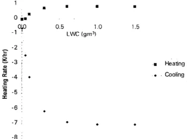
•The heating and cooling rates both increase with increasing Lwe

due to an increase in the cloud optical depth. Figure 2.8 shows the peak heating and cooling values for each Lwe. From this plot, both curves approach a constant value when LWe exceeds 1.0g/m3•The heating rate approaches a maximum of 0.9 Klhr and

the cooling rate approaches a minimum of -7.0 Klhr.

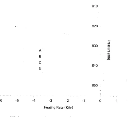
The effect of the distribution of cloud water on heating and cooling is investigated next. The cloud for this simulation is 300 meters thick cloud with a base at 1.5 km and an equivalent liquid water path of 30g/m1. The liquid water is distributed so that the

maximum water is at the top, bottom or middle of the cloud or evenly distributed as shown in figure 2.9. Figure 2.10 shows the heating and cooling profiles. The strongest cooling occurs when the largest amount of water is located at cloud top (distribution A). The next highest cooling occurs when the liquid water is evenly distributed (distribution D). When the maximum amount of water is at the base of the cloud (distribution B), the cooling rate is lowest and peaks below the cloud top. The peak cooling rate also occurs below the cloud top when the maximum amount of water is in the middle of the cloud (distributionC). Distributions Band D cause the highest heating rates which occur nearer to the base of the cloud. The heating that results from distributions A and e is stretched out over a larger portion of the cloud. Heating occurs at the highest level in the cloud when the maximum amount of water is at the top of the cloud.

~~::::::::~~---Height(km) 2 3 4 5 _ _ _ 7 ... .9 6 4 2 o -2 -4 -6 I. 200 300 400 . :Q 500 . .§. e 600 :::s II) II) ell Q: 700 800 900 1000 . -8 Heating Rate (Klhrl II. 200 300 400 :Q 500 .§. ~ 600 :::s II) II) ~ a.. 700 800 900 1000 +.~ .. -8 -6 -4 -2 0 2 Height (krn 2 3 4 5 _ _ _ 7 ., _____ 9 4 6 8 Heating Rate (Klhr)

Figure 2.5: _{Change in heating rates with heightfor a 300 meter thick cloud with a}

_rwe

010.2 g/m3 (Case I) and 0.6 g/m3 Case II).

550 650 ~ • "'I:l o _ _ '-o"o"o"o"ooo".o.-.".""00"00" 00 00"0"0"0"0"0"""" ":. ". """" I ~ - I : _~-_-_-_-_-_- -~_-_-- J

1

~ 3 ~ -8 07 -6 -5 -4 ·3 ·2 -1 0

Heating Rate(KIM

Thickness (ni 200 300 400 500 600 - - - 1 0 0 0 - - - - 1500 "000" _.2000 -0_0_3000

Figure2.6:Heating and cooling rates when the thickness ofthe cloud is changed. Cloud base is

• x o 81Qtl -ttl 820 ---_... Xltl ..,

I

;~_c 830

~

; "3 .!'!: ttl

I

840[E: liJ

--_.----_

.. LWC Igm'3) 0.01 0.05 0.1 0.3 0.6 1.0 1.5 850 $ -8.0 -7.0 -6.0 -5.0 -4.0 -3.0 -2.0 -1.0 9J 0.0 1.0

Heating Rate (K/hrI

Figure2.7: Heating rates for a range ofLWCfor a cloud with a base at 850 mb and a top at 820

mb.

•

•

•

•

o ••

•

o~o 0.5 1.0 1.5

-,

, LWC (gm3) -2 -;:-.<:: _:+ ~ -3

_•

Heating Ql 1a _{. Cooling} Cl:: _-4 • • Cl c 1a _-5 Ql ::r: -6 • -7 • _{• •} -8

820 825 830 . A :a g B ~ 835 . C

=

'"'" D l!! _{840 .} D.. 845 . 850 .. 0 0.1 0.2 LWC(gm3)

Figure 2.9: Different distributions ofcloud liquid water for a 300 meter thick cloud with a liquid water path of30 g/m2.

810 820 " ;; 830 _'"'" A :;CD B '3 ~ C 840 D 850 -6 -5 -4 -3 -2 -1 o

Heating Rate (Kihr)

2.3 Liquid water retrieval using passive microwave 2.3.1 Theory

The microwave spectrum is defined from 3 GHz (10 cm) to 1000 GHz(OJ mm). There are absorption lines for water vapor and molecular oxygen in this range which make microwave remote sensing useful for measuring atmospheric water content; however, a problem with using microwave sounding is that emissivity values of the earth's surface vary from 0.4 to 1.0 in the microwave region. Most microwave retrieval methods to determine water vapor and cloud liquid water can only be used over the ocean where the emissivity typically only ranges between 0.4 and 0.5, although a method that uses a combination of IR and microwave data has been developed to determine cloud liquid water over land [Jones and Vonder Haar, 1990].

The ocean appears cold at microwave frequencies but the overlying atmosphere and cloud layer increases the emitted radiation as viewed by a satellite. Column

integrated water vapor (called precipitable water) and cloud liquid water can be determined by measuring the change in the emission.

The presence of ice or precipitation can alter the retrieved microwave radiance. Ice scatters radiation at microwave frequencies if the ice particles are large compared to the wavelength of the incident radiation. Raindrops and cloud drops larger than 100 greatly absorb and scatter microwave radiation. Therefore, retrieval of cloud liquid water is not as accurate for precipitating clouds and high clouds, such as cirrus, that contain ice.

2.3.2 Description of method

The total amount of water contained in an atmospheric column is determined from a physical retrieval method [Greenwald and Stephens, 1995] that uses passive microwave measurements of brightness temperatures. This method, hereafter referred to as the Greenwald method, employs simple, vertically integrated forms of the radiative transfer equation with minimal empiricism that is used only for calibration purposes. The method simultaneously computes the liquid water path and water vapor content for a

non-precipitating, ice-free, oceanic region given microwave vertical and horizontally polarized brightness temperatures, infrared brightness temperature and sea surface temperature.

The brightness temperature measured by a microwave radiometer is a function of atmospheric transmittance and surface emissivity. In the microwave region, Planck radiance is directly proportional to temperature, which is known as the Rayleigh-Jeans distribution. Thus the radiative transfer equation can be written as

The first term is the emission from the surface, the second term is the integrated atmospheric emission, and the last term is the downwelling radiation emitted by the atmosphere that is reflected by the surface and retransmitted to the satellite. The equation contains the atmospheric transmission function, t, polarized surface emissivity,8₅,

In the microwave spectrum, the surface emissivity varies considerably over land depending on the moisture content of the soil and type of vegetation. Over the ocean, the surface emissivity varies with surface roughness, salinity and amount of sea foam. The Greenwald method currently is valid only over the ocean. The surface emissivity is calculated from existing models that use microwave brightness temperatures and sea surface temperature as input.

Assuming an isothermal atmosphere and absorption by water vapor in the boundary layer only, equation (2.40) can be simplified to

(2.41 ) The square of the atmospheric transmission function contains the transmission factors for oxygen, cloud liquid water and water vapor.

.., ., ") ")

"C-

=

"C~"C;"C~ (2.42)

The transmission factor for water vapor is a function of the water vapor absorption coefficient, viewing angle and water vapor content.

(2.43)

The transmission factor for cloud liquid water is a function of the absorption coefficient for liquid water, viewing angle, and liquid water path.

The transmission factor for oxygen depends on temperature and is determined by the empirical equation

"Cox =a+bI;, +cT,; +dT;

To solve for W and L, equation (2.41) is first used to obtain the horizontally and

(2.45)

vertically polarized brightness temperatures. The difference between the brightness temperatures is

{,H V\.2 2 2

11TH

=

T,\£ - E , W "CL "Cox

Substituting equations (2.43) and (2.54) into equation (2.46) and rearranging

(2.46)

(2.47)

Equation (2.47) is then applied to two microwave channels, such as the 19 GHz and 37 GHz channels, to provide a set of linear equations

w

=

"C\Km -1"2KII9 8 L

=

1"2K wl9 -1"IK w37 8 where, (2.48) (2.49) (2.50) (2.51) (2.52)

Thet) and t₂physically represent optical depths of the atmospheric water in non

-precipitating regions and excluding ice. The T₁₇ and ~9 values compensate for the

CHAPTER 3 DATA

3.1 Case selection

Two areas of study were selected for this research, one in the equatorial warm pool of the western Pacific Ocean and one in the subtropic region of the eastern Atlantic Ocean. Marine cases were necessary because the Greenwald method [Greenwald, 1995] for calculating liquid water is valid only over the ocean. Data for the first case were available for mUltiple sites which allows for the investigation into the spatial heating rate gradients. The second case consists of only one site, so heating rates were analyzed over the course of one day.

3.1.1 Case I

The first case was selected with the intent of using data from the Tropical Ocean and Global Atmosphere Coupled Ocean-Atmosphere Response Experiment (TOGA COARE) because of the extensive data collected during this field experiment. TOGA COARE was conducted in the region of 145°E to 155°E and 50_{S to SON from November}

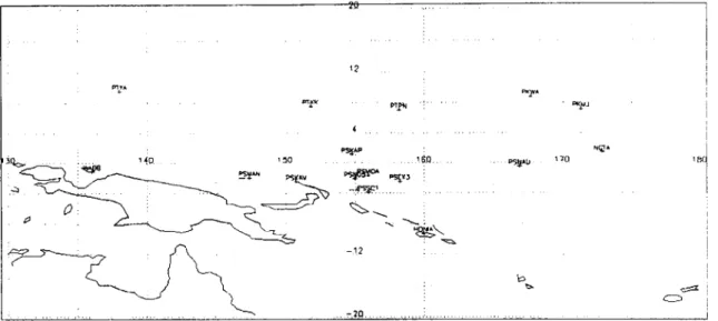
1992 to February 1993 to study ocean-atmospheric processes in the western tropical pacific. TOGA COARE data sets used here were the 6 hourly balloon soundings from islands and research ships and half hourly visible and infrared images from the GMS satellite. Figure 3.1 shows a map of this region with rawinsonde launch sites identified.

"'1" ., .

,

.

no.

-.1.2

..~.~Q.

Figure3.1: Location ofrawinsonde sounding sites in the TOGA COARE region.

,

I

I

I~I

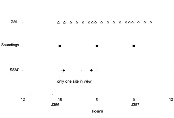
Calculation of radiative heating rate requires knowledge of the distribution of cloud layers and their liquid water content as well as the vertical temperature, pressure and humidity profiles. Since SSM/I is used to measure the liquid water path, the primary cases for analysis must coincide with DMSP overflights of the region. The selected SSM/I data set consists of microwave data collected on 1356 from 2303Z to 231 OZ. The nearest GMS IR and visible images are from 1356 at 2315Z. Analysis is further limited to the areas immediately surrounding sites where rawinsondes were launched because the soundings are the only means of determining the vertical cloud structure in this case. As shown in figure 3.2, the closest sounding data are available for 1357 at OOOOZ,

GM Soundings SSM .

•

....

•

•

•

•

12

only one site in view

18 J356 o Hours 6 J357 12

Figure3.2: Timeline ofthe satellite and rawinsonde data retrieval timesfor December 21-22,

1992 (J356-J357).

The primary analysis time for which the heating and cooling rates are computed is established as OOOOZ (10:00 am, local time) on1356. Heating and cooling rates are also

computed six hours earlier and six hours later using the rawinsonde and IR data to determine the vertical cloud profile but the same liquid water amount fromOOOOZ

because SSM/I data is not available. The exception is that SSM/I data is available only for PSMOA at 1800Z.

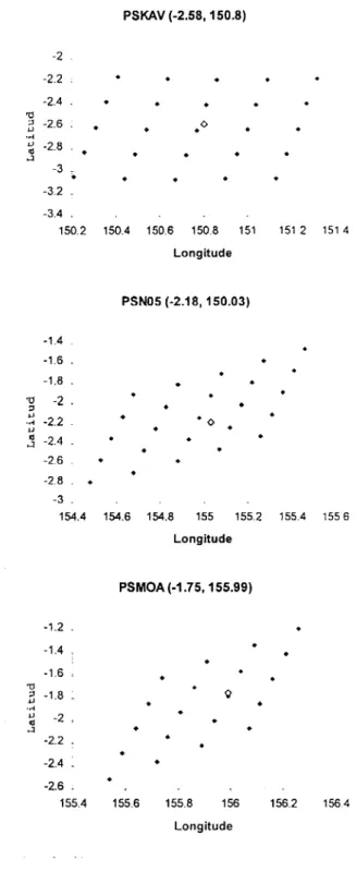
Three sounding sites were selected based on their proximity to each other and because the rawinsonde data were available every 6 hours The selected sounding sites are: the island of Kavieng (PSKAV) and the research ships Xiangyanghong 5 (PSN05) and Moana Wave (PSMOA).

The resolution of the data is limited by the SSM/I 37 GHz channel which has a resolution of 37 km x 29 km. The location of each sounding site is shown relative to the nine nearest data points in figure 3.3.

PSKAV (-2.58, 150.8) -2 -2.2 -2.4 'tl ;1 _-2.6 lJ ... lJ _-2.8

'"

...:l -3

•

-32 -3.4 150.2 o

.

150.4 150.6 150.8 151 1512 1514 Longitude PSN05 (-2.18, 150.03) -1.4 -1.6 . -1.8 . -2 . _• '0 ;1 lJ ... -2.2 . " j -2.4 . -2.6 . -2.8 . -3 . 154.4 154.6 154.8 · 0 155 155.2 155.4 1556 -2 • -1.2 . -1.4 . -1.6 , 'tl E-1.8 . ... lJ <l ...:l -2.2 . -2.4 , Longitude PSMOA (-1.75, 155.99) • • _• -2.6 ; 155.4 1556 155.8 156 156.2 156.4 Longitude

3.1.2 Case II

Case II looks at a single cloud layer in a subtropical marine region. The area selected was studied in the ASTEX (Atlantic Stratocumulus Transition Experiment) phase of FIRE (First ISCCP Regional Experiment). This field experiment occurred during the month of June 1992 on Porto Santo, an island in the Madeira Islands located at 33.08 ON latitude and 16.35 oWlongitude in the north Atlantic Ocean. A map of the

island and location of the experiment site is shown in Figure 3.4.

Figure 3.4: Map ofthe ASTEXregion [from Huebert, et al.. 1996}.

ASTEX was chosen because of the high occurrence of single layer stratus clouds that transition to stratocumulus and because of the extensive ensemble of in situ and

remote sensing instruments. A description of the instruments and data sets can be found in Cox et al. [1993].

, The surface observation and remote sensing data sets acquired from ASTEX include rawinsonde, ceilometer, microwave radiometer, and Doppler 8.7 mm radar. Satellite data consists ofIR and visible images from the European Meteosat-3 satellite and microwave radiometer data from SSM/Ion the DMSP satellite. The availability of these data sets for June 14 (1166) is shown in figure 3.5. June 14 was selected for analysis based on ground observation reports of overcast, non-precipitating conditions.

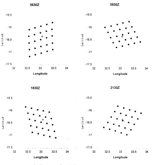
Cloud liquid water path and infrared data are gridded based on the resolution of the 37 Ghz channel on the SSM/I instrument which is 37 km x 29 km. Figure 3.6 shows the proximity of these gridded data points to Porto Santo.

RADA.

Ceilometer ,x X!-x ; x i-X -X - X , X : X - X • X - X - X --x . x - x - x - x - x - x x - x - x • x

f"kteosat _*-ts¥A-ts-4sl:>.

*'

l:>.~A *,-A-Al:>.Al:>.Al:>.Al:>.A A Al:>.Al:J.l:J.l:J.l:J.l:J.Al:J.l:J.l:J.Al:J.l:J.l:>.*,l:J.

*'

l:>.t;s.l:J.

, ' Soundings _ 1 ,.- ! : , !

.-

-.

'.

'.

' SSM' I

.-. ! : , ··,·t··..·t···:···t·· • • . : - C' +

•

-.

o 1 2 3 4 5 6 7 8 9 10 11 12 13 14 15 16 17 18 19 20 21 22 23 0 Hours

0630Z 0930Z -15.5 -15.5

•

•

•

•

•

-16

_•

•

-16

•

•

_•

•

•

_•

•

_•

_•

•

_•

•

•

'tl

•

•

•

'tl

•

OJ _<> OJ

•

<>

•

1.1

•

1.1

•

•

... -16.5

• •

... -16.5

•

1.1 1.1

• •

•

l\J

•

•

l\J

•

..:l

•

..:l

•

•

•

•

•

•

•

-17

•

-17

• •

•

-175 -17.5 32 32.5 33 33.5 34 32 325 33 33.5 34 Longitude Longitude 1830Z 2130Z -15.5 -15.5

•

_•

•

_•

-16

•

•

-16 .

• •

•

•

• •

_•

•

_•

•

'0

• •

'0

•

•

"

•

<> OJ

•

_~

•

1.1

•

•

1.1 -16.5 ... -16.5

•

...

•

•

1.1

•

1.1

•

•

l\J

•

•

l\J

•

•

>-1

•

>-1

•

•

_•

•

•

•

•

_•

•

-17

•

-17

•

•

_•

-17.5 -17.5 32 32.5 33 33.5 34 32 32.5 33 33.5 34 Longitude Longitude

Figure 3.6: Locations ofsounding site relative to gridded data points for the different analysis

3.2 Satellite data sets 3.2.1 SSMII

The microwave brightness temperatures used to compute the column integrated liquid water are obtained from the Special Sensor Microwave/Imager (SSM/I) flown on the Defense Meteorological Satellite Project (DMSP) satellites. The satellites are referred to as F-8, F-lO, and F-11. Data for this project was obtained from the F-lO and F-11 satellites. The DMSP satellite is in a sun-synchronous orbit at an inclination of 98.8°. The SSM/I instrument performs a conical scan with a 53° viewing angle between the

instrument line of sight and nadir. Both vertically and horizontally polarized radiation is measuredat 19.35 GHz, 37 GHz, and 85.5 GHz while only vertically polarized radiation is measured at 22.235 GHz. Table 3.1 identifies the resolution of each channel.

Table 3.1:Spatial resolution ofthe SSM/! channels on the DU')P satellite.

Channel

I

Frequency(GHz)

I

Resolution(km) 1 19.35 V 69 x43 2 19.35H 69 x43 3 22.235 V 50x40 4 37V 37x28 5 37H 37x29 6 85.5 V 15 x 13 7 85.5 H 15 x 13

Channels 1 through 5 are used to compute the liquid water path as described in section 2.3. Spatial resolution increases with increasing frequency; therefore, the 37 GHz channel

has the smallest resolution of the 5 channels. The 37 GHz channel has 37 km along-track and 29 km cross-track resolution.

The SSM/I brightness temperatures for each channel are obtained from Wentz formatted data. The Wentz format converts the radiation measured by SSM/I into brightness temperature and includes the earth location of each pixel in latitude and longitude coordinates.

3.2.2 GMS

The visible imagery and IR brightness temperatures for Case I are obtained from a Geostationary Meteorological Satellite (GMS). The GMS-4 is a spin-stabilized, Japanese satellite in geostationary orbit located at 140oE. The satellite contains a Visible and Infrared Spin Scan Radiometer (VISSR). The visible channel (0.5 ~m-0. 75 ~m) has a resolution of 1.25 krnat the satellite sub-point and the infrared channel (10.5 ~m -12.5

~m)has a resolution of 5.0 krn.

The IR data are used as input into the Greenwald method to determine an average cloud temperature. In addition, the IR and VIS data are used to analyze the cloud scene as described in section 2.1.1. TheIRdata are also used to indicate cloud top temperature and

the height of the highest cloud layer.

3.2.3 Meteosat

Data from the European Space Agency geostationary meteorological satellite, Meteosat-3, was used for CaseII. The Meteosat satellites detect radiation in three spectral

and 10.5 Ilm - 12.5 Ilm for the thermal infrared band. Data from the visible and infrared bands were utilized for this research. The visible imagery has a spatial resolution at the sub-satellite point of 2.5 km and the infrared imagery has a resolution of 5 km.

As with the GMS data, the Meteosat infrared imagery data was input into the Greenwald method to determine the cloud liquid water and the visible and IR imagery was used to identify the cloud scene.

3.2.4 Sea surface data

Sea surface temperature (SST) fields were extracted from a weekly averaged, one-degree, gridded, global data set. The SST data set blends skin temperatures retrieved from the Advanced Very High Resolution Radiometer (AVHRR) flown on polar orbiting satellites with SST from ship and buoy observations [Reynolds and Smith, 1994].

3.3 Satellite data set remapping

The microwave, infrared, and sea surface data sets needed to compute cloud liquid water come from different sources and projection spaces. The Polar Orbiter Remapping and Transformation Application Library (PORTAL) [Jones and Vonder Haar, 1992] is used to remap the data to a common projection space prior to computing the cloud liquid water using the Greenwald method.

The concept of PORTAL focuses on processing each data set into a generalized data format (GDF). Once a data set is in GDF format it can be remapped to match the projection space of another data set, also in GDF format, by merging the two GDF files.

and associated earth-location information from the original data set. The header contains information about the type of data and allows the user flexibility to handle conditions like missing data and multiple channels. The data is structured into scan lines to accommodate the time and earth-location of each data point.

For this project, the IRand Sea Surface Temperature (SST) data sets were remapped into the projection space of the SSM/I data set.

CHAPTER 4 CASE I

4.1 Analysis of clouds in scene

4.1.1 Cloud type from satellite VIS and IR imagery

Manual inspection of the visible and IR images for 2345 Z on 1356 (figures 4.1 and 4.2, respectively) reveal the cumuliform type clouds that are typical in the tropics. Widespread deep convection south of the rawinsonde sites is related to the ITCZ. Deep convective clouds are identified by very high albedo (white) on the visible image and low temperature (inverted to appear white) on the infrared image. An overlying cirrus layer exists over large portions of the area, appearing white with a wispy texture in both. The storm to the southwest of PSKAV is dissipating, as evident by the cirrus blowoff. Two of the sites, PSN05 and PSMOA, are located near some small dissipating convective storms with a layer of cirrus above. The island site, PSKAV, appears to be located in a more an area of broken cloudiness as evident by warmer, lower level clouds.

4.1.2 Vertical cloud structure over selected sounding sites

Satellite imagery only shows the top layer of clouds. The base of the cloud and any intervening layers are determined here using sounding data from each of the selected sites. The cloud layers are determined from the rawinsonde humidity profile using the threshold method described in section 2.1.2. To supplement these data, the average IR

Figure 4.1: GMS visible image for J356 at 23152.

Figure -1.2: GMS infrared image for J356 at 23152.

brightness temperature is used in conjunction with the rawinsonde profile to determine the height of the top of the highest cloud layer. This averaged cloud top is used for situations where the RAOBS indicate a cloud top that extends to temperatures lower than -40°C since humidity measurements are unreliable at these temperatures.

The vertical humidity profile for each site and time is shown in figure 4.3 with an overlay of the vertical location of the cloud layers.

4.2 Liquid water retrieval

4.2.1 Horizontal distribution of liquid water over scene

Figure 4.4 is a plot of the column integrated cloud liquid water path computed for 1356 using the Greenwald method and microwave images from SSM/I and infrared images from GMS. The measured liquid water paths are shown scaled from 0 kg/m" to 0.32 kg/m2.White is used within the SSM/I swath to correspond to liquid water paths

greater than 0.32 kg/m2and includes areas where the 37 GHz signal is saturated due to rainfall or the presence of land.

The intensely cloudy areas of the visible and infrared images in figures 4.1 and 4.2 compare well to the areas that contain the highest amounts of liquid water content. The storm regions to the northwest of PSN05 and PSMOA and over the island south of PSKAV (New Britain) have liquid water paths exceeding 0.32 g/m2;however, most of the

37 GHz signal is saturated here due to the presence of rainfall or land. Areas that have less cloud liquid water correspond to the clearer regions of the GMS imagery. There is good correlation between the nearly zero liquid water and the clear areas north and south

PSKAV 1800Z PSN051800Z PSMOA 1800Z 12 12====- 12 = 10 . 10 . 10 . .Q 8 . .Q 8 . .Q 8 '" 6. u 6 . u 6 . ..c ..c ..c 01 01 CI ... ... ... QJ _{4 .} QJ _4. QJ ₄ :r: :r: :r: 2 , 2 2 . O~ o . o . 70 80 90 100 70 80 90 100 70 80 90 100 110 RH(%) RH(%) RH(%) PSKAVOOOOZ PSN050000Z PSMOAOOOOZ 12 1 2 > 12 10 . 10 . 10 .Q 8 . _.Q

'0

.Q 8 . '" 6 . _" 6 . .J 6 ..c ..c ..c CI 01 01 ... ... ... QJ _{4 ..} QJ ₄ QJ _4. :r: x >- :r: 2 2~

2~

=-O==- O = - o . 70 80 90 100 70 80 90 100 70 80 90 100 RH(%) RH(%) RH(%) PSKAV0600Z PSN050600Z PSMOA0600Z 12 .. 12 12 10 , 10 . 10 .Q 8 . _.Q 8 . _.Q 8 .J _{6 ,} u ₆ " ..c ..c ..c 01 CI CI ... ... ... QJ 4 . QJ ₄ QJ ₄ x x x ~ 2'7' 2 ..

~

o

r::::=====r

o :_. . 70 80 90 100 70 80 90 100 80 90 100 RH(%) RH(%) RH(%)

.0206 .10 .14 .18 .22 .26 .30 >.32 kglm 2

150 152 154 156 158

There is much uncertainty to the retrievals of liquid water in the tropics due to the presence of rain and thick cirrus associated with areas of tropical convection. A reliable measurement of cloud liquid water is not possible when rain is widely distributed within the field-of-view of the SSM/I instrument.. Raindrops greatly absorb microwave radiation with the absorption characteristic depending much more on the size distribution of the drops than it does with drops of radius less than 100 Ilm. Raindrops interact with microwave radiation mostly outside of the Rayleigh regime, so scattering also becomes important. The ice in thick cirrus clouds also impacts the liquid water measurements because ice scatters microwave radiation.

4.2.2 Vertical distribution of liquid water

An average of the 25 pixels surrounding each site is used as the observed columnar amount of liquid water over that site. This water amount is then distributed among the layers of clouds according to the height and type of cloud observed through

sounding and satellite data. Cloud height is used to decide whether the cloud contains only water or a mixture of water and ice. A cloud layer with a temperature above O°C consists of water only. Supercooled water can exist in clouds at temperatures below O°C but the likelihood of ice increases as the temperature decreases. As seen in figure 4.5, the fraction of clouds that contain ice approaches 100% at -20°C; therefore, cloud layers that

exist between O°C and -20°C can be considered mixed water/ice clouds and clouds at temperatures below -200

e

consist almost entirely of ice. Since ice scatters microwave length radiation, the ice water content is not determined from SSM/I data. The amount of

Figure4.5: Likeliness of ice with cloud temperature [from Rogers and Yau. J994]

ice in the clouds is calculated here using an empirical formula that relates ice water content to temperature [Liou, 1986]

In(IWC)

=

-7.6+4 exp [-0.2443 x 10-3

~71-

20

YW]

(4.1 ) The type of cloud gives an indication of the approximate liquid water content that it should have. Many observational studies have used aircraft to measure the droplet size distribution in various types of stratiform and cumuliform clouds [Paltridge, 1974 and Slingoet al., 1982, for example]. The size and number concentration of drops determines the liquid water content, or mass of cloud water per unit volume, according to

LWC

=

~1tp

I

r

r3n(r)dr

3

J

6r (4.2)

wherePI is the density of water. A summary of the drop size distributions determined by various investigators is shown in table 4.1.

Table 4.1: Drop size distribution and LWCfor different clouds [from Liou. 1992]

A method for distributing water among the cloud layers is now described. Clouds are first categorized as water clouds, mixed water/ice, or ice clouds by temperature only. A cloud that covers two categories is split into those two types of cloud. For example, a cloud with a base temperature above

a°C

and a top temperature below

a°c

is split into a water cloud up to the

aoc

level and a mixed waterlice cloud above that level. Next, the liquid water profile is computed using the height of the cloud and an initial, reasonable value for the liquid water content. Liquid water path is integrated liquid water content

w=

~dz

(4.3)

where w is the liquid water content in g/m' and !1z is the thickness of the cloud in meters. The liquid water content is adjusted until the total liquid water path from each cloud equals the total liquid water path. Figure 4.6 shows the distribution of liquid water that is

used for the clouds at each site and analysis time. These cloud heights and liquid/ice water contents are key inputs to the heating rate calculations as shown earlier in section 2.2.5.

One condition that was shown in the sensitivity study but not considered here is that liquid water is highly variable within a cloud. In a cumulus cloud, the amount of liquid water peaks in the upper half a cloud, with smaller amounts at the base and top of the cloud [Pruppacher and Klett, 1978; Starr and Cox, 1985; and Spinhirneetat., 19891.

Although this vertical profile of liquid water within a cloud is important to accurately compute heating and cooling rates [Stephens, 1978], a constant-height distribution of liquid water is used here because this investigation looks at the change in heating rates integrated over 200 mb layers.

a) 100 200 300 _{02 .027} 022 .0 _{400 027i~~_J} 8 014 014 500 .04 c-_______.J OJ

"

09 .05 ;j _{600 .1} .07 OJ OJ OJ ₇₀₀ ;, 0.. 800 . 900 . 1000 . 150 151 152 153 154 155 156 157 Longitude b) ₁₀₀ 200 300 _{02 .025} .0 _{400 .} ==:::J014

=

.04 OJ 500 .16 ---I

"

15 ::J ₆₀₀ to 07 OJ OJ ₇₀₀

"

0.. 800 900 . 1000 150 151 152 153 154 155 156 157 longitude c) ₁₀₀ 200 .009 _.011 300 t=:=.l 027

~~:

n

.0 ₄₀₀ 035

0

.055 Ei OJ 500 _{06 2}

"

.15 =-~:::J ::J _{600 .} to to I1J 700 . ;, n. 800 ₀₅ 900 . 1000 , 150 151 152 153 154 155 156 157 longitude

4.3 Heating and cooling rates 4.3.1 Analysis

The LWBAND program is used to calculate the infrared heating and cooling rates for each site and analysis time. This program computes the net flux and heating rate with a vertical resolution of 10mb. The net flux is dependent on cloud optical depth which is a function of cloud thickness and the Lwe or IWe of the cloud. There was only one time

(OOOOl) that all three sites were in the field-of-view of the SSM/I during the selected

analysis time period; therefore, only data from this time is available to compute the LWP. The vertical profiles of the heating and cooling rates for each site and analysis time are shown in figures 4.7 through 4.9. Sharp peaks in heating or cooling rate occur at the cloud base and top, respectively, for each layer. The largest cooling rate (-100 oK/day) and heating rate (35 oK/day) occur for the single-layer, mixed waterlice cloud over

PSN05 at OOOOZ. The heating and cooling profiles for the multiple-layer and divided

single-layer clouds have maximum heating and cooling rates that nearly balance each other. The maximum cooling rates for these clouds range from -20 TO -30 oK/day, and the heating rates range from 15 to 30 oK/day.

In most of the multiple-layer cloud cases, the peak cooling rate for the lower cloud layers is less than the peak cooling rate of the top layer. This suggests that the upper cloud increases the downwelling infrared flux that is incident on the lower clouds, which decreases the net flux and reduces the cooling rate of the lower clouds.

The abrupt changes in heating rate within the divided single-layer cloud layers result from the division of the cloud into the distinct water, mixed, or ice regions. A more

appropriate scheme would be to gradually change the water content with height in the cloud according to the microphysics of the cloud.

PSKAV 200 PSN05 200 400 400 '1:l 'U '1 '1 (I) (I) en en en en 600 ~ 600 ~ ro ro 3 3 tr tr 800 800 1000 -30 -20 -10 0 10 20 30 dT/dt (Klday) PSMOA 1000 -30 -20 -10 0 10 20 30 dTidt (Klday) 200 400 '1:l Ii (I) en en 600 ~ (I) 800 -30 -20 -10

o

_ 1000 10 20 dTidt (Klday)

PSKAV 200 PSN05 200 400 400 "CI 'U t1 ,~ ro ro til til til til 600 ~ 600 ~ ro ro 8 3 tr tr 800 800 dT/dt (Klday) -30 -20 -10

o

10 1000 20 PSMOA 1000 -100 -80 -60 -40 -20 0 20 40 dT/dt (Klhday 200 400 "CI 'i ro til til - 600 ~ ro 3 tr 800 1000 -30 -20 -10 0 10 20 30 dT/dt (Klday)

PSKAV 200 PSN05 200 400 400

""

""

ti ti co co rn rn rn rn 600 ~ 600 r:ti co co :J :J 0- 0-800 800 dTldt (Klday) 1000 -30 -20 -10 0 10 20 30 dT/dt (Klday) PSMOA -30 -20 -10 200 400

""

ti co rn rn 600 ~ co :J 0-800 o 10 1000 20 i . 1000 -30 -20 -10 0 10 20 30 dT/dt (Klday)

The local, abrupt changes in the heating profile are averaged out when the heating and cooling rates are integrated over a 200 mb atmospheric layer. Figures 4.10 through 4.12 show the integrated heating and cooling rates for each site and analysis time. These plots reveal the vertical atmospheric heating or cooling for the observed cloud scene. Most noticeable are the vertical gradients between the 200-400 mb layer and the 400-600 mb layer for every analysis time which are due to the heating differential between the cloud top and base. On average the cloud top in all the cases is located in the 200-400 mb layer and the cloud base is located in the layer below. The thermal difference between the two layers causes turbulent motion which destabilizes the cloud.

The effect of radiative heating on overall diabatic heating is considered when. based on the magnitudes of latent and sensible heating, radiative heating and cooling variations are at least ±0.2 °K/day/200 mb [WCRP-86, 1994]. Looking at the three analysis times, the highest layer of the atmosphere (200 - 400 mb) experiences cooling rates that range from 0.26 OK /day to 0.63 OK /day. This is not surprising since most of the cloud tops are located here. The 400 - 600 mb and 600 - 800 mb layers have net heating or net cooling, due to the variety of cloud conditions that exist in this region. The magnitude of heating/cooling is small though, less than ±0.2 OK/day everywhere except PSN05 at 0000 Zwhere the cloud top is below 400 mb. This situation also results in a

horizontal heating gradient, from PSN05 to PSMOA, that could have an impact on the atmospheric dynamics in this area. The lowest layer has a small amount of cooling at all sites except PSMOA at 0600Zwhere the base of the low cloud here provides radiative

IR cloud top tem perature 10 _Longitude 0 -10 150.5 151 151.5 151.9 152.4 152.8 1533 153.6 154.1 154.4 154.8 155.2 1555 155.8 U -20 tl1 -30 Ql 'd -40 -50 -60 200-400 m b layer PSN05 PSMOA PSKAV 02 '@ 0 0 0 _-0,2 N "-~ -0.4 'd "--0,6 if -0,563 -0.53 -0.634 -0,8

PSKAV 400-600 m b laye r PSN05 PSMOA

0.2 0,125 0.063 E 0

.1.

...

0 _,0.043 0 _-0.2 N "-~ -0.4 'd "--0.6 :<: 0 -0.8 0.2 600-800 mb layer 0.083 0.129 0.023

I

'@ 0

•

0 PSKAV PSN05 PSMOA 0 _-0.2 N "->, -0.4 III 'd "-if -0.6 -0,8

PSKAV 800-1000 mb layer PSN05 PSMOA

0.2 'oj 0 0 -0.059 -0.045 0 _-0.2 -0,082 N "-~ -0.4 '0 "--0.6 :>::: 0 -0.8