Parallel Convolutional Neural NetworkArchitectures for ImprovingMisclassifications of Perceptually CloseImages

(1)

M

ÄLARDALENS

H

ÖGSKOLA

A

KADEMIN FÖR

I

NNOVATION

,

D

ESIGN OCH

T

EKNIK

V

ÄSTERÅS

,

S

WEDEN

Thesis for the Degree of Master of Science in Engineering

Dependable System 30.0 credits

Parallel Convolutional Neural Network

Architectures for Improving

Misclassifications of Perceptually Close

Images

Al-Mustafa Khafaji

Aki15002@student.mdh.se

Examiner: Masoud Daneshtalab

Mälardalen University, Västerås, Sweden

Supervisor: Håkan Forsberg

Mälardalen University, Västerås, Sweden

(2)

Abstract

:

Deep Neural Networks (DNNs) have proven to be an alternative for object identification for multiple application areas. They are treated as a critical component for autonomously

operating systems and consequently crucial for many companies. Since DNNs do not behave in the same way as traditional deterministic systems, there are several challenges to cope with before being used in safety-critical applications. Both random and systematic failures must be taken care of, including permanent and transient faults, design faults in hardware and

software, and adversarial inputs. In this thesis, we will be constructing an architecture that is robust and can detect misleading errors produced by a DNN to some extent. One way to cope with failures in DNNs is through architectural mitigation. By adding redundant and diverse architectures, it can detect misclassification to a greater area. Convolutional neural network architectures will be tested and trained using MATLAB and Simulink. The focus will be on fault-tolerant architectures. The method used in this thesis is experimental research. The results show that parallel architectures can detect misleading image classification better. In addition, and somewhat unexpected, combining three different networks gives worse results than combining two networks.

(3)

List of symbols

ANN – Artificial Neural Network CNN – Convolutional Neural Network DNN – Deep Neural Network

EDMN – Error Detection Mitigation Network FFNN – Feed Forward Network

FGSM – Fast Gradient Sign Method FI – Fault Injection

FLM – Fault Logic Modeling GRU – Gated Recurrent Unit

GTSRB – German Traffic Sign Recognition Benchmark Data (I-FGSM) – Iterative Fast Gradient Sign Method

ILD – Interstitial Lung Disease IMDS – ImageDatastore

LSTM – Long Short-Term Memory MR - Miss Rate

NN – Neural Network

PA – Predictive Augmentation

PMA – Predictive Multiple Augmentation RA – Random Augmentation

RELU – Rectified Linear Unit RNN – Recurrent Neural Network RELU – Rectified Linear Unit RSR – Road Sign Recognition SPOF – Single Pount Of Failure SVM – Support-Vector Machines

T-FGSM Targeted Fast Gradient Sign Method TMR – Triple Module Redundancy

TPDCNN – Two Parallel Deep Convolutional Neural Networks UPN – Unsupervised Pretrained Network

(4)

1. Introduction

Deep Neural Networks (DNNs) have proven to be an alternative for object identification for multiple application areas. They are treated as a critical component for autonomously operating systems and, consequently, necessary for many companies [1]. Due to their outstanding performance in many benchmark problems and applications, DNNs have become a popular research area in the machine learning domain [4].

Fault tolerance is an essential property for real-time applications with high-reliability requirements along with low power consumption and high performance. For example, aircraft flight control system and onboard avionics depending on it. The price of recognition errors is very high. It can be challenging for critical applications such as autonomous driving, which requires uninterrupted computation for a long time. They use Deep learning techniques for object recognition and detection in real-time.

Image classification is an essential part of digital image analysis. It is interesting to have an architecture that is robust, fault-tolerant, and accurate for detecting objects. For example, in the real world, the test images can come from data assessments different from those in training. It can be challenging where the data can disagree in viewing angels, object scales, and camera properties [5].

Since DNNs do not behave in the same way as traditional deterministic systems, there are several challenges to cope with before being used in safety-critical applications. In the avionics industry, both random and systematic failures must be taken care of, including permanent and transient faults, design faults in hardware and software, and adversarial inputs (the alteration of inputs that force a trained DNN to misclassify). One way to cope with failures in DNNs is through architectural mitigation. By adding redundant and diverse architectures, image misclassification can be detected to a greater extent [2].

Cat and ocelot are used in the image experiments because these two animals are perceptually close to each other, making it harder for the networks to classify them correctly. We also chose these animals because it will be tough for humans to type them correctly when both animals standstill. After all, they are very identical to each other when they are not moving.

This thesis concerns constructing an architecture that is robust and fault-tolerant to detect misleading errors from a DNN. Multiple CNN architectures will be tested because there are already pre-trained architectures. Still, the focus will be the fault-tolerant architectures using MATLAB and Simulink to implement and model them. The method that will be used in this thesis is experimental research, and through this method, the questions in the problem formulation will be answered.

(7)

2. Background

This section consists of fundamental concepts and describes the theory needed for understanding this thesis.

2.1. Dependable Systems

A dependable system is one that is trustworthy to its users. It requires that the system be highly available while ensuring a high degree of service integrity within a period. The service delivered by a system is its behavior as it is perceived by its user(s); a user is another system; it can be physical and human that interacts with the former at the service interface.

2.1.1. Dependability can be divided into three factors

[22]

:

1. Attributes: a way to assess the dependability of a system.

Dependability includes as special cases such as attributes/properties such as: a) Availability: ability of the system to deliver services when required. b) Reliability: ability of the system to deliver services as specified. c) Safety: ability of the system to operate without catastrophic failure.

d) Security: ability of the system to protect itself against deliberate or accidental intrusion.

e) Resilience: ability of the system to resist and recover from damaging assets. 2. Threats: an understanding of the things that can affect the dependability of a system. The threats:

a) Faults: is the adjudged or hypothesized cause of an error.

b) Errors: is the part of the system state that may cause a subsequent failure.

c) Failures: a failure occurs when an error reaches the service interface and alter the service.

3. Means: ways to increase a systems dependability The Means:

a) Fault prevention: how to prevent the occurrence or introduction of faults. b) Fault tolerance: how to deliver correct service in the presence of faults. c) Fault removal: how to reduce the number of severity of faults.

d) Fault forecasting: how to estimate the present number, the future incidence, and the likely consequences of faults.

2.1.2. Fault Tolerance

As explained before Fault tolerance is intended to preserve the delivery of correct service in the presence of active faults. It is mostly implemented by error detection and subsequent system recovery. It uses backup components that automatically take the place of failed components, ensuring no loss of service. Creating a fault-tolerant system aims to avoid disruptions arising from a single point of failure, establishing the high availability of mission-critical applications or systems [22].

Several systems or components which is a single point of failure can be made fault tolerant using redundancy. Fault tolerance follows typically one of these models:

(8)

1. Normal functioning which means that a fault tolerant system encountering a fault may continue to function as normal, without any change in throughput, response time or other performance metric.

2. Graceful degradation: some of the fault tolerant systems will experience "graceful degradation" in performance when facing certain errors. So, a small fault will have a small impact rather than major impact or even causes the system to fail.

These are the elements of a fault tolerant system:

1. Hardware system: that are backed up by identical or equivalent systems. For example, a server can be made fault tolerant by using an identical server running in parallel,with all operations mirrored to the backup server.

2. Software system: backed up by other software instances. Software can be designed to be fault tolerant so that it can continue to operate even when an error, exception, or invalid input occurs, if it has been designed to handle such errors rather than defaulting to reporting an error and halting

3. Power source: that are made fault tolerant using alternative sources. For example, many organizations have power generators that can take over in case main line electricity fails.

2.1.3. New technologies in dependable systems

Safety concerns become more difficult to tackle when complex automation problems emerge from deep learning or machine learning. Many technologies are employed in the automotive industry, to monitor the vehicle's environment, such as cameras, radar, sensors, and lidar. The sensor data is fed to algorithms that support various functionalities, which may be of high relevance to safety. These algorithms may also be highly complex, making them difficult to analyze [30].

A Machine learning algorithm in the self-driving car is a continuous rendering of the surrounding environment and predicting possible changes to those surroundings. One of the biggest challenges in machine learning algorithms for autonomous driving is to develop an image-based model for prediction and feature selection. Sometimes it isn't easy to detect and locate because the system's images are not clear. It might be blurry and hard for the classification algorithms to miss the object and fail to classify. It is also challenging to implement an image recognition and analytics model when the manufacturer needs an accurate dataset containing hundreds or even thousands of images [29].

2.1.4. Image Processing

Digital image processing is to process images by computer. It can be defined as subjecting a numerical representation of an object to a series of operations in order to obtain a desired result. It mainly includes image collection, image processing and image analysis. A digital image processing system is comprised of three components [23]:

1. Computer system to process images on. 2. An image digitizer.

3. An image display.

Image processing mainly include the following steps: 1. Importing images via image acquisition tools. 2. Analyzing and manipulating the image

(9)

3. Output in which result can be altered image or report which is based on analyzing that image.

One of the phases that image processing has that interests us is object detection and

recognition, which is a process that assigns a label to an object based on its descriptor [23].

2.1.5. Transfer learning

Transfer learning is a machine learning method that uses information from one model to obtain another one on related tasks or domains. Transfer learning provides the advantage of reducing the cost of creating models, and the transfer learning works in understanding of the model features which is learned from the first task. Transfer between jobs, between input types, and between input domains are some of the many variants of transfer learning [34]. Some of the new risk added that can affect the learning are [34]:

• Performance verification • Negative transfer

• Transfer from publicly available models • Correct optimization target

• Transfer algorithms

There are many methods to perform transfer learning, some of these methods can be classified into:

• Supervised (requires labels)

• Semi-supervised (partially requires labels) • Unsupervised (not requiring labels)

The methods usually have trade-offs between the amount of data necessary and the

complexity added on top of the original learning algorithm. Unsupervised would be a good choice if the domain gap is small enough.

2.1.6. Object Detection

Object Detection is a crucial output of deep learning and machine learning algorithms. It is the process of finding instances of objects in images. In deep learning, object detection is a subset of object recognition, where it does identify not only the item but also identifies the location of an object in an image. The main goal is to teach a computer the level of understanding of what an image or a video contains. Two approaches can be used to get started with object detection. One of them is to use a pre-trained object detector, and the other is to create and train a custom object detector. A first approach is an approach that enables the user to start with a pre-trained network and then change the user’s application. This will help the user to get faster results because the object detectors have already been trained on

thousands or millions of images [24]. The algorithms of object detection act as a combination of image classification and object localization, it takes an image as input and produces one or more bounding boxes with the class label attached to each bounding box.

For machine learning there are also techniques that are used for object detection, some of these techniques are [24]:

1. Aggregate channel features (ACF).

2. SVM classification using histograms of oriented gradient (HOG) features. 3. The Viola-Jones algorithms for human face or upper body detection.

(10)

2.2. Deep Neural Network (DNNs)

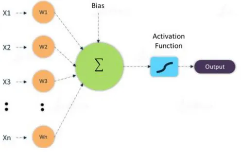
A DNN is an acyclic graph consisting of connected computational units, referred to as neurons, arranged sequentially in a series of layers. The neurons in the layers are connected through edges, and each edge has a corresponding weight. The neurons possess weights and bias, and they are altered during the learning phase to learn intended functionality. The weights symbolize the connection strength between the neurons. These parameters help activate the neuron, and each neuron is activated using functions such as rectified linear unit RELU, sigmoid, tanh, etc [19].

As shown in the figure below, the inputs are multiplied by the corresponding weight the sum of the weighted inputs and bias are given as inputs to the transfer function.

Figure 1. Artificial Neural Network architecture with one neuron.

Neural Network (NN) is produced to replicate the activity of human brain in processing data and making pattern for use in decision making. The data in DNN flows from the input to the output layer without going back, in this case the DNNs are called Feedforward Networks (FFNNs). The links between the layers as showed in figure 2 have one direction and it is forward direction, in another words it means that the link are one-way links.

Figure 2 shows a Neural Network (NN) that consist of three different layers: input layer → hidden layers → output layer.

(11)

Figure 2. Diagram of Deep neural Network Alicia Lozano-Diez (CC BY 4.0) [7].

The input layer in the DNN is provided with an input x of dimension D. X input will be transported by the hidden layers hj. Output O provides the output of the DNN for the target class. DNN that are feedforward and used to do a classification task can have the following structure. An input layer, that is provided with some input vectors to represent the data, two or more hidden layers, and an output layer, which calculate the output of the DNN. The output in the last layer is compared to the reference label. The error criterion is used to calculate the cost. Weight matrices Wj,j−1 and bias vectors bj are the parameters that defines the model in figure 2, where j going from 1 to the number of hidden layers. These parameters are adapted to minimize a cost function. In equation 1 a given training set with (x(i)_,_y(i)₎_where_x(i)_{is a feature} vector and y(i) _{its corresponding class. The transformation function takes the W and the b vector} into account, which connect one layer to its previous one, and the equation gives the activation values of neurons.

[7]: ℎ_𝑗(𝑥(𝑖)_{) = 𝑔(𝑊}

𝑗,𝑗−1ℎ𝑗−1(𝑥(𝑖)) + 𝑏𝑗), 𝑗 = 2, … . . , 𝑁 − 1 (1)

ℎ₁(𝑥(𝑖)_{) = 𝑔(𝑊}

0,1𝑥(𝑖)+ 𝑏1)

In the following equation the output layer calculates a softmax function for a classification task, there it outputs the probability P of a given input x to be classified to a certain class. There hl(x) indicate to the last hidden layer for input x, and C are the total number of classes. W_𝑙𝑐_{𝑎𝑛𝑑 b}

𝑙 𝑐

in the equation indicate the W matrix and b vector and connect the output unit for class with the last hidden layer [7].

[7]: 𝑃(𝑐|ℎ(𝑥))= exp (𝑊𝑙

𝑐_ℎ

𝑙(𝑥)+ 𝑏𝑙𝑐)

∑𝑐_𝑘=1exp (𝑊𝑙𝑘ℎ𝑙(𝑥)+ 𝑏𝑙𝑘)

(12)

Developers usually start with a set of annotated experimental data, when it comes to implementing a DNN application. They divide it into three sets [8]:

• Training: to create the DNN model in supervised settings.

• Validation: to tune the model’s hyper-parameters (configuration parameters that can be modified to better fit the expected application workload).

• Evaluation: to evaluate the accuracy of the trained model.

When it comes to image classification, DNN can be trained in any of the following settings: • Single-label classification

• Multi-label classification

Single-label classification: Each datum is associated with a single label l from a set of disjoint labels L à |L| > 1. The classification problem is called binary classification problem if |L| = 2, and if |L| > 2 then it is a multi-class classification problem. MNIST, CIFAR-10/CIFAR-100, and ImageNet are some of the popular image classification datasets.

Multi-label classification: where each datum is associated with a set of labels Y à Y ⊆ L. some of the popular image classification datasets in multi-label classification are COCO and imSitu, where COCO can be labeled as a car, person, traffic light, and a bicycle. All of the things that COCO can label; a multi-label classification supposed to predict from a single image that shows all these kinds of object [8].

Here are some examples of the network architectures in DNN: • Unsupervised Pretrained Network (UPNs)

• Convolutional Neural Network (CNN) • Recurrent Neural Network (RNN) • Recursive Neural Network

This thesis is interested in CNN architectures, because CNN is the top choice for a such thesis that handle about image classification and computer vision, and try to improve the state of the art.

2.3. Convolutional Neural Network (CNN)

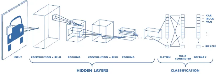
The goal of CNN is to learn higher-order features in the data via convolutions. They are mostly applied to analyzing visual images and state the art of image classification, segmentation, object detection, and other image processing tasks. It consists of layers with local spatial connectivity and sets of neurons with shared parameters. The use of CNN architecture will reduce the hardware for storage and make the training process fast even if the parameters are very high, unlike other architectures out there. CNN has the capability of taking raw inputs and identified features from these raw inputs. As shown in figure 3, each neuron in the input layer is connected to neurons in the hidden layer in typical neural networks. However, in a CNN, only a small region of the input layer is connected to neurons in the hidden layer, as shown in figure 3 [9] [10] [6].

(13)

Figure 3. Architecture Convolutional Neural Network (Courtesy of : www.mathworks.com).

There are three ways to train CNNs for image analysis [13]: 1. Training the model from scratch

2. Using transfer learning

3. Using pretrained CNNs to extract features for training a machine learning model. The architecture of CNNs consist of two major functional modules which are [18]:

1. Feature learning and extraction module: Feature module is composed of exchanging convolution and pooling layers along with activation function.

2. Classification module: uses multi-layer Perception (MLP) along with Rectified Linear Unit (ReLU).

2.4.1. Convolution operation

Convolution is one of the main building blocks of CNN where convolution layers perform 2D convolution operation on x(height*width*depth*) input image with the convolution filter kernel Cf (height*width) to the product feature map.

They are executing the convolution by moving the filter over the input. These filters are the weight of the features and are adjusted during training; they move in strides (strides determine the number of the convolution operations and the distance between two scanned regions) [15]. Matrix multiplication is performed at every location and sums the results onto the feature map [11] [12].

The output size of a convolution layer can be estimated as in the equation below: [17]: 𝑜𝑢𝑡𝑝𝑢𝑡 = 𝑖𝑛𝑝𝑢𝑡 − 𝑟𝑒𝑐𝑒𝑝𝑡𝑖𝑣𝑒 𝑓𝑖𝑒𝑙𝑑 + 2 ∗ 𝑝𝑎𝑑𝑑𝑖𝑛𝑔

𝑠𝑡𝑟𝑖𝑑𝑒 + 1 [1]

Here is an example of convolution operation in 2D using 3x3 filter. Where the green area is where the convolution operation take place, it is called receptive field. A receptive field of a

(14)

single neuron is the specific region of the retina, in which something will affect the firing of the neuron. Padding is rows or columns of zero added to the borders of an image input so that the feature map will not shrink. Because the size of feature maps is always smaller than the input, by using padding, you can control the output size of the layer [15] [14]. Stride specifies how much we move the convolution filter at each step [20]. The receptive field in figure 4 is 3x3 due to the size of the filter [15].

Figure 4. Performing convolution operation by sliding the filter over the input [15]. In figure 4, it shown that the filter (the green area) are in the top left, and the output of the convolution operation is 4 as shown in the Feature Map.

Next is moving the filter to the right as shown in figure 5, and do the same operation, adding the result of the next operation to the Feature Map.

Figure 5. Next step of the convolution operation by moving the filter to the right [15].

experiment continue like this as shown in figure 6, and collect the convolution

results in the feature map.

(15)

2.4.2. Pooling

After the convolution operation comes the pooling layers which helps in reducing the spatial sample size of input feature map, based on an overlapping square max kernels

Mk(height*width) [11] [12].

Pooling layers down sample each feature map independently, reducing the height, and width, keeping the depth intact.

The most common type of pooling is the max pooling as shown in figure 7, where it takes max value in the pooling window. It works opposed to convolution operation, where it moves a window over its input and takes the max value in the window.

Figure 7. max pooling takes the largest values [15]. The four important hyperparameters when using CNN are [15] [14]:

• The kernel size.

• The filter count (how many filters do we want to use). • Stride (how big are the steps of the filter).

(16)

2.5. Fault Tolerant Neural Network

The fault tolerance property of neural network assures that the neural network will continue to operate even in the presence of faults and degrades gracefully over time. According to the definition of 𝜖-fault tolerance, a neural network N performing computations HN is said to be

fault tolerant if the computation HNfault performed by a faulty neural network Nfault is close to

HN.

‖𝐻_𝑁(𝑋) − 𝐻_{𝑁𝑓𝑎𝑢𝑙𝑡}(𝑋)‖ ≤ 𝜖

For 𝜖 > 0 and input image X is sampled from the training dataset D. The value of 𝜖 has to be 0 for the neural network to be completely fault tolerant 𝜖 = 0.

Fault tolerance can be classified into active and passive fault tolerance. The design of active fault tolerance is complex as it includes the implementation of detection and localization components within the system. it provides a system the ability to recover from faults by reallocating the task performed by faulty elements to the fault free one. meanwhile a passive fault tolerance does not react in any special way to compensate for the effect of internal faults, the design of passive fault tolerance is to mask by compensation a given maximum number of faults.

By using passive techniques, we can achieve higher degree of fault tolerance than active techniques, because the active approaches can’t cover all possible cases [16].

2.5.1. Physical and Transient faults in NN

Physical fault in a neural network can be mapped to errors so that it can estimate the fault tolerance for a given architectural implementation. The mapping is required to show the error analysis's instability and consistency in evaluating the actual fault tolerance of a system's physical implementation. Stuck -at model allows for the examination of fault tolerance at the behavioral level, separately from the actual performance or detailed characteristics of material faults. This model has proved to be tolerable to model many material faults. It abstracts and simplifies faults into stuck-at values affecting single components.

A transient fault may only persist for a short period, and it is often a result of external disturbances. There are two types of transient faults Intermittent and Timing. The intermittent fault recurs with some frequency, and they are more challenging to detect than permanent ones. The timing faults change the timing behavior rather than the structure of the circuit. The faults affect circuit parameters, which define the timing characteristics of the device.

Random bit-flip model is intended to model transient faults that regularly happens at register or memory elements. The damage under this model is done only to the data and not to the circuit itself [16].

2.5.2. Adversarial Attacks

An adversarial attack consists of modifying an original image so that the changes are almost undetectable to the human eye but the network changes its output to something else. In this case, the image is called a negative image. Some of the severe attacks for the real-life application are modifying a traffic sign to be misinterpreted by an autonomous vehicle, causing an accident.

(17)

Most successful attacks are gradient-based methods. The attackers modify the image in the direction of the gradient of the loss function concerning the input image [25]. There are two approaches to perform this attack:

• One-shot attack: the attacker takes single step in the direction of the gradient. • Iterative attack: here the attacker takes several steps instead of one.

The adversarial attack is classified into two categories, targeted attacks, and untargeted attacks. Where targeted attacks, the attacker pretends to get the image classified as a specific target class, and untargeted attacks are to enforce the model to misclassify the adversarial image. Some other common attacks are where the first 2 of them are one shot attack and the third one is iterative attack:

• Fast gradient sign method (FGSM)

• Targeted fast gradient sign method (T-FGSM) • Iterative fast gradient sign method (I-FGSM)

The most common defense against adversarial attacks consist of introducing adversarial images to train a more robust network [25]. One more approach was been proposed by Chow et al. in 2019 in the paper titled “Denoising and Verification Cross-Layer Ensemble Against Black-box Adversarial Attacks”, where the approach focused on enabling machine learning system to automatically detect adversarial attacks, and then automatically repair them by using denoising and verification ensembles [26].

2.5.3. Data input distortions

Recent advances in DNN have enabled autonomous driving systems to adapt their driving behaviors according to the dynamic environment. Most of the real-world data are taken during the daytime and in the right weather conditions. Using end-to-end supervised learning, the framework made it possible to train a DNN to predict driving behavior by inputting driving scenes using the driving scenes and action. Some of the latest techniques show that adding error-inducing inputs to the training dataset can help improve the reliability and accuracy of existing autonomous driving models. Real-world driving scenes can hardly be affine-transformed and captured by the cameras of autonomous driving systems; the blurring/ fog/rain effects made by merely simulating the corresponding results. The rain can be affected by adding a group of lines over the original image because this rain effect transformation is more distorted than the fog effect transformation. After all, when there is rain, the camera tends to be wet, and the image is possible to be blurry. But other conditions be simulated easy, for example, snowy road condition requires different sophisticated transformations for the road and the roadside objects [27].

2.5.4. Untrained input data

There are a lot of issues in the domain of autonomous driving. Some of these issues can be that the system has been trained and tested on the roads in a country with very organized traffic and deployed for driving on roads in another country with terrible driving conditions. S. Shafaei et al. had proposed one approach that targets the problem related to differences in training and operational conditions. The approach aims to detect how far away the input from the system was trained on. If the data point is significantly different from the original data, then the system is expected to enter a fail-safe mode. Else normal operation continues. Another issue can be that the vehicle which employs this system want to overtake another car in front of it. In some countries, the driving rules state that one must overtake only one side, either left or right. In

(18)

autonomous vehicles, there is no guarantee that the system has learned these rules and follow them. In the same paper, as mentioned before, they proposed using ontologies to enforce such conditions. Ontologies are a way to model the entities and relations in a system. The theories stored in ontologies will be internally translated into machine-readable first-order logic, making it more straightforward to describe constraints that the system must obey in the environment. Inputs to the component and outputs generated thereby will be tested against the set of environmental conditions to ensure that they are fulfilled; if not, the system enters a fail-safe mode [28].

2.5.5. Reduced false negatives

False-negative reduction in machine learning means that the outcome where the model incorrectly predicts the negative class is reduced. For example, the model inferred that a particular email message was not spam (the negative type), but that email message as spam. It is considered to be a negative value if the negative value is incorrectly classified. One approach to reducing the false-negative rate is proposed by R. Chan et al. [32] by applying a maximum Likelihood decision rule that adjusts the neural network’s probabilistic /softmax output with the prior class distribution estimated from the training set. In this way, fewer instances of rare classes are overlooked but to the detriment of producing more false-positive predictions of the same class.

2.5.6. Reduced false positives

False positive reduction in machine learning means that the outcome where the model incorrectly predicts the positive class is reduced. For example, the model inferred that a particular email message was spam (the positive class), but that email message was actually not spam. The reduction of false positive rate (FPR), which is measured by the proportion of negatives that are incorrectly identified as positive. For example, some research was done to compare the effect of two types of networks: CNN and DNN on the task of false positive reduction in juxtapleural lung nodule detection [31]. Where they designed a two-phase framework, in the first phase a CNN based classifier is used to detect juxtapleural lung nodule. In the second phase they perform false positive reduction for the detected nodules based on two types of network, DNN and CNN, respectively. Some of the difficulties that they had to perform the nodule detection is that the juxtapleural nodules in their dataset is very small. They generate both positive data and negative data where they take positive samples from a point within the nodule area and negative within the non-nodule area and divide them into training and testing data. The results showed that CNN is more efficient and automatic, Both CNN and DNN have shown their efficiencies in the task of false positive reduction, and that DNN performs slightly better than CNN in the experiments that they done in their research.

(19)

3. Related work

The following section describes the related work and state-of-the-art in the field of using neural network in dependable applications.

3.1. Adversarial Fault Tolerant Training

V. Duddu, V. Rao, V. Balas [21] have in their research shown the evaluation of neural networks trained using the proposed training algorithms for different classification tasks, where they proposed a scalable and efficient training approach for fault tolerant neural networks for state-of-the-art image recognition tasks. The proposed training algorithm for their research combines Feature Extractor network with an unsupervised learning objective of identifying and extracting the dominant and robust features in the input image. The objective of training the Feature Extractor in unsupervised fashion is to achieve robust features with a smooth distribution. And the Classifier Network with a supervised objective to predict the image label given the extracted features.

The training algorithm evaluated on two major benchmarking datasets:

1. FashonMNIST: it is similar to MNIST dataset and consist of 60,000 samples and test set of 10,000 examples, and each data sample is a 28x28 grayscale image associated with a label from 10 classes.

2. CIFAR-10: consist of 60,000 images, with 50,000 images for training and 10,000 for testing, where each datapoint is 32x32 colored images. The images are clustered into 10 classes representing different objects.

Four architectures with different network depth and complexity are considered to evaluate the scalability. Two different architectures are chosen and trained for each dataset. The two architectures that they used for FashonMNIST are a fully connected deep neural network as architecture 1 where it comprises of three hidden layers (512, 1024, 514) with ReLU, and for the second architecture they used a convolutional neural network which includes two convolutional layers of 20 and 50 filters with 5x5 filters, and two maxpool layers of kernel size 2x2 stride of 2. For CIFAR-10 architecture 1 includes convolutional layers with number of filters as [64, 128, 256, 512, 256, 128, 128] with LeakyReLU activation with scaling factor of 0.1, where for architecture 2 they used a smaller network with three convolutional layers with numbers of filters [64, 128, 128], with kernel size 3x3 and stride of 2.

In their results they showed comparison of highly generalized model (low generalization error), the model has low inference accuracy, and high generalization using a combination of unsupervised and supervised learning in an adversarial setting which strongly regularizes the model, resulting from the proposed Fault Tolerant Training Algorithm with commonly used regularization functions: Lasso (results in sparse parameters which allows to prune certain nodes or weight) and Tikhonov (results in a tradeoff between model test Accuracy and Generalization Error). For architecture 1 in FashonMNIST has about 1,82x lower generalization, and for architecture 2 shows 1,9x higher generalization. For the second dataset they showed for architecture 1 shows a higher generalization of about 2.7x using the proposed approach while about 3x superior generalization in Architecture 2 compared to the corresponding unregularized model. This showed that the proposed adversarial Fault Tolerant Training approach resulted in strongly generalized neural network classifier compared to neural network using Lasso and Tikhonov regularization functions [21].

(20)

3.2. Improving image classification robustness

M. Nyberg, J. Gustavsson, S. Rehman and S. Harisubramanyabalaji [11] have performed a research about improving image classification robustness by using predictive data augmentation, where they validated their framework on two different training datasets (German Traffic Sign Recognition Benchmark Data (GTSRB), collection of 2d camera on autonomous bus), and with 5 generated test groups, to show their results in overall classification accuracy. The two techniques that they used for adapting the dataset for improved robustness with high confidence in classifying traffic signs were Predictive Augmentation (PA) and Predictive Multiple Augmentation (PMA). Predictive Augmentation (PA) and Predictive Multiple Augmentation (PMA) methods are proposed to adapt the model based on acquired challenges with a high numerical value of confidence. They went with a simple CNN architecture rather than a deep layer model. The architecture that they used for traffic signs is LeNet-5. In their results, they showed that the risk range accuracy had got incredible improvement in both PMA and PA compared to the other two Without Augmentation (WoA) and Random Augmentation (RA). The classification accuracy for the collected GTSRB and heavy vehicle data have delivered 96% and 86%. It also showed that the PA and PMA improved the overall classifier accuracy by 5-20% in both datasets, among the five different test groups [11].

3.3. Efficient On-Line Error Detection and Mitigation for Deep Neural

Network Accelerators

C. Schorn, A. Guntoro and G. Ascheid [2] have performed a research about Efficient On-Line Error Detection and Mitigation for Deep Neural Network Accelerators, they perform fault injection simulation with two deep neural network and data sets. They classify their methods with random bit-flip injections in the activation of two different classification networks. The first classification network is an All-CNN which only uses convolutional and fully connected layers and is trained on the CIFAR-10 classification benchmark, which consist of 32x32 pixel RGB images that are divided into 10 different classes. The second classification network is Road Sign Recognition (RSR) network trained on the GTSRB which contains RGB images of 43 different types of sign traffic, where for the RSR network they considered two different cases, the first one is classification of a single independent road sign images by DNN accelerator, and the second one where they consider the RSR network is the processing sequential input data. They used an Error Detection Mitigation Network (EDMN) with 256 neurons on both networks, in each of the first two fully connected layers. In each of the experiment the EDMN is optimized using stochastic gradient descent. The sequential-RSR is more realistic for a real-world application, since a driving car captures several sequential images while approaching a road sign. In this case they expected that the EDMN can distinguish between the changing resulting from slight modifications of the input image and the changes resulting from a random bit-flip. In the experiment that they performed, they showed that the results are better for the RSR experiments, because the RSR network shows better classification performance than in All-CNN on CIFAR-10.Their error detector achieved a recall of up to 99,03% and precision of 97,29 %, while requiring a computation overhead of only 2,67% or less in the RSR-sequence, where EDMN can recover the correct classification for at least 62% of the test samples in this case, because without the EDMN in place the samples would led to wrong image classification and therefor the classification accuracy would be 0 [2].

(21)

3.4. Medical Image Classification with Convolutional Neural Network

A research by Q. Li, W Cai, X. Wang, Y. Zhou, D. Feng and M. Chen [3] has been performed about medical image classification using CNNs. They have designed a customized CNN with shallow convolution layer to classify lunge image patches with interstitial lung disease (ILD). The architecture had an input of a normalized lung image patch with unit variance and zero mean. The first layer in the architecture is a convolutional layer with kernel size of 7x7 pixels and 16 output channels. The second layer is a max pooling layer with 2x2 kernel size. The other three layer are fully connected neural layers with 100-50-5 neurons in each layer . The training samples are divided into 10 groups. Every time they test samples from one group is chosen as the testing data, and the other sample from the remaining 9 groups are used as a training data. To get the final results they needed to do 10 testing sessions and each time with different group as the testing data. They also used Random image shifting on the training data to increase the number of the training samples to avoid the over-fitting issue.

As for the results, they compared their classification results with three different feature extraction approaches which are SIFT feature with key point located at the patch center; rotation-invariant LBP feature with three resolutions; and unsupervised feature learning using RBM, and all the three approaches are coupled with SVM classification models, while theirs customized CNN method does not have an classifier as SVM, instead their classification model is learned by the three fully connected neural network layers, and they have not compared with the other approaches based on customized feature design specifically for the ILD images. Their results showed that the customized method that they did, achieved better classification performance than the other three approaches. Their method also exhibits large performance margin over the popular feature descriptors. They also concluded in their results that the method is capable of extracting discriminative features automatically without manual feature design and achieving good benchmark performance [3].

3.5. Parallel Deep Convolutional Neural Networks for Pedestrian

Detection

In a research that have been performed by B. Lin and C. Chen [33] about presenting a deep learning approach that combines two parallel deep CNN models for pedestrian detection by using two CNN, and each network is capable of solving a particular mission-oriented task to form parallel classification.

By using GoogLeNet as one of the two CNN, because it is a flexible deep learning architecture consisting of the early layers (for learning early representations), middle layers (for deep feature extraction), and final layers (for integration and classification), and for the second network they will introduce another CNN with different missions assigned. To form their pedestrian detection, they combine the two CNN, and mixing the final layer classification. This approach will be called Two Parallel Deep Convolutional Neural Networks (TPDCNN). The model in their architecture is reduced to a concise network with fewer inceptions in the middle layer, and they also retrained the early layers and final layers to make the training process easier and faster. The TPDCNN has two rows that each row has a separated model. The rows are upper row and lower row of the TPDCNN. The first one consist of the early layers, middle layers of 2 inceptions and final layers,to train this model, they used all of the available positive (pedestrian) samples and negative (background) samples, meanwhile for the lower row it has a different

(22)

mission, where it focuses on a more difficult goal, where harder negative samples can be separated with the positive ones in the learned feature space. Their results shows that the miss-rate MR is closer on the upper row when the number of inceptions in the middle layer is 2 or 3. They also showed the detection quality on different deep architectures and their TPDCNN, where the GoogLeNet structure is not really good in pedestrian detection compared to other structures, their upper row model achieved better and more favorable performance than GoogLeNet. The lower-row model can achieve comparable performance of the upper-row model. By using bounding-box regression, both models can perform better and achieve better results. They also compare their TPDCNN to the other pedestrian detection approaches using deep learning, AlexNet is one of these methods. Their results show that TPDCNN achieved better MR 19,57 % with the bounding box regression, which performs more favorable than the other competitive deep learning methods for pedestrian detection [33].

(23)

4. Problem formulation

If DNNs are used for object detection in safety-critical applications, the DNN itself should be robust and capable of correctly detecting objects to a very high probability. However, to be accepted in safety-critical applications, the whole system must ensure that the likelihood of misclassification of images is extremely low. The SVM algorithm can be used for the analysis of misclassification.An SVM is a non-parametric classifier that finds a linear vector to separate classes, and for the fitcecoc it can fit multiclass models for support vector machines or other classes. Classification error means that the classifier is not able to identify the correct class of the test tuple. To reduce the frequency of misclassifications, the DNN can be trained in different ways with different data sets of objects, but it can never be trained with all possible inputs. Therefore, the suggested solution is to use monitors (both in time and space) monitoring the DNN in the form of redundant and diverse hardware or software. There are many ways to train a DNN; it can be trained using a pre-trained model or designing the model from scratch. The dataset of the objects will be divided into training and validation set.

In this thesis, the following questions will be addressed:

• How can the number of misleading classifications of perceptually close images be reduced by using parallel convolution architectures (CNN architectures)?.

• What are the differences between pre-trained networks and normally trained (from scratch) networks in terms of detecting misleading classifications?

(24)

5. Method

The process that will be followed to answer the questions in the problem formulation is to do a background research in the beginning and based on the research outcome an experimental research will be done.

The first task will be the background research about DNNs and the classes that DNNs have and understand how they work. A pre-study will be performed to get all the theory needed to provide insight to the reader, so the reader will understand what DNN is about and background research of the related work to understand the state-of-the-art methods that DNN have. The main goal of background research is to help with the idea of the second task.

The second task will be the thesis's idea, which is to focus on redundant and fault-tolerant architectures that can detect misleading errors. This task will help analyze and evaluate the algorithms used in modeling and implementing the task.

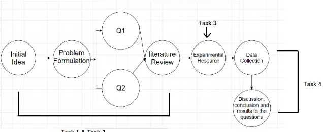
The third task will be experimental and modeling and implementing the CNN architectures using MATLAB and Simulink. See figure 9; the simulation will find a fault-tolerant, accurate, and robust architecture. The output from this task will help answer our second question in the problem formulation, where the fourth task will be analyzing the data that we will get from the third task and drawing the right conclusions, and in the fourth task, answer to question 1 and 2 will we get.

Figure 9. Method process.

5.1. Data collection

The source for references and basis for the background research is scientific articles and papers. The literature is collected from the most well-known article databases such as IEEE, etc.

5.2. Methodology

This section contains the specific techniques that are used to identify, select, process and analyze information about this research.

(25)

5.2.1. Analysis

It requires a systematic approach to analyzing patterns and problems in a set of literature. To identify important literature studying will help us getting a bigger picture of the research itself, and identifying concepts leading to the state-of-art.

5.2.2. Justification

A literature analysis provides the positioning of this thesis context to the state-of-art. It also provides a comprehensive understanding of the study that this thesis is all about. Two animals that look alike will be selected by downloading them from Google, and 200 images of each animal will be our dataset. We will look at three different networks which 2 of them are pretrained and one is trained from scratch.

In the first experiment, the network will learn from AlexNet, a convolutional neural network trained on more than a million images. Our classifier will be using transfer learning. Transfer learning is the process of taking a deep neural network that is already being trained and repurposed on a second related task, which in this case, AlexNet is the network. Using transfer learning, we can get the results that we want with much less effort than doing it from scratch because we are building on work that is already being done.

The first experiment will go on loading the data image in an imageDatastore (imds), where each individual image fits in memory, and inside the imds there are the 2 files that contain the location of the images. Test cross-validation is done to randomly split the data in 80% training data and 20% validation data using hold-out method which is the state-of-art cross-validation technique used in machine learning [35]. After splitting the data by cross-validation, we are downloading the pre-trained network (AlexNet) from the deep learning toolbox in MATLAB by using the command “net = AlexNet”, where the using of this model suits us because CNNs have 2 parts, one is the features extraction and the second one is the classification.

AlexNet is a 25-layer model. Layers 1-23 contains extraction and layers 24-25 are classification layers. The next two steps are to train the SVM classifier and to validate the Testset. A confusion matrix is used to plot the results.

In the second experiment, instead of using AlexNet, we define the convolutional neural network architecture by specifying the size of the images in the input layer and the number of classes in the fully connected layer. The next step after defining the CNN architecture is to train the network and specify the training options. The last step is the same as the first experiment, i.e., A confusion matrix will be used after the classification of the validation set.

In the third experiment, which is almost the same as the first, we use another pre-trained network instead of the one we had in the first experiment. ResNet18 will be used. ResNet-18 is a pre-trained network on more than a million images and can classify images into 1000 object categories, such as keyboard and many animals. This experiment will go on loading the images as an image datastore automatically labels the images based on folder names and stores the data as an ImageDatastore object. This will help us store large image data, including data that does not fit in memory. the data will be divided into training and test data in the same way as the previous experiment. Loading the pre-trained network will be the next move after storing the data. ResNet18 requires input images of size 224-by-224-by-3, so to automatically resize the

(26)

training and test images before they are input to the network, augmented image datastores were created.

The network creates a hierarchical representation of input images. Deeper layers consist of higher-level features, created using the lower-level features of earlier layers. To get the feature representations of the training and test images, activations was used on the global pooling layer, 'pool5', at the end of the network. The global pooling layer pools the input features over all spatial locations, giving 512 features in total. Extracting the class labels from the training and test data will be next, then after that we going to use the feature extracted from the training images as predictor variables and fit a multiclass SVM using fitcecoc. The last two steps are the same as the other experiments, where confusion matrix going to be used after the classification of the validation set.

The confusion matrix will be used in the last step in all the experiments to display the total number of observations in each cell. The rows of the matrix correspond to the true class, and the columns correspond to the predicted class. Diagonal and off-diagonal cells correspond to correctly and incorrectly observations, respectively.

We will be changing the relationship between trained data and test data to ensure that we will get an error rate, by using these methods; first method is to change the test data (validation set). The second method is to add more picture to the input. We will do so because it is more important to increase the misclassification.

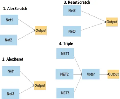
When we are done with implementing and testing all the three networks and comparing them with each other, and after seeing the results they gave us, the networks will be combined in parallel, as you can see in figure 10. First, we are going to look at each network individually and see the results of each one. After that, we will combine them and decide on it.

The first combination is Net1+Net2, which have both AlexNet (Net1) and trained from scratch network (Net2) combined parallel to each other. The second combination is Net1+Net3, and this combines both AlexNet (Net1) and ResNet (Net3). The third combination will be Net2+Net3, and it is between ResNet (Net3) and trained from the scratch network (Net2). As for these combinations, both networks need to classify the same image identically for the system to output a result. Otherwise, a fault detected/image mismatch will be sent out. That is, an output will be sent out if the images are correctly classified but also if both networks misclassify the same image in the same way.

The last combination will be Triple by combining all the networks Net1+Net2+Net3, and having a voter at the end. The only way to get an output from this combination is through having two networks agree on the classification. It doesn’t matter if the two agreed networks have classified the image correctly or incorrectly. In all other cases, a fault detected/image mismatch will be sent out.

(27)

Figure 10. Combination of all networks

5.2.3. Validity threats

Poor datasets with not enough data or poor variety of images. in this case are threats to the accuracy, and robustness. To mitigate this threat, we going to use large datasets with large variety of images, it shall include different colors, because these things can affect the accuracy of detecting an image.

(28)

6. Results

This section contains the experiments result from testing and training different CNN architectures in MATLAB. The first experiment will show the results by taking a pre-trained network AlexNet and adjusting it to our data by using SVM algorithm and misclassification learner. The second experiment is about training a network from scratch and using misclassification learner to show the misclassification error rate. The third experiment will show the results by taking a pre-trained network ResNet-18 and adjusting it to our data, in the same way as the previous experiment.

6.1. AlexNet

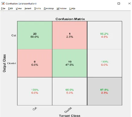
This experiment will go on loading the data image in an imageDatastore (imds), where each image fits in memory, and inside the imds, there are the two files that contain the location of the images. Test cross-validation is done to split the data into 80% training data randomly, and 20% validation data using the hold-out method, the state-of-art cross-validation technique used in machine learning. After the training section, a pre-trained (AlexNet) model is loaded. This model suits us because CNNs have two parts: the features extraction and the second one is the classification. The input images to AlexNet are a colored image of size 227x227x3 selected from Google and resized; this means all the images in the training set and all test images are 227x227x3. The results will be different almost every time we run the code because it will take random images on each test. First, we tested with 100 images of each animal, and later we added 100 more images to each one to see if there are some differences in the results. Figure 11 shows the results of using 100 images of each animal and 20% in each animal's validation set (cat and ocelot) and 80% training data. It misclassified a cat for ocelot 0 times and misclassified an ocelot for a cat one time.

Figure 11. Results from AlexNet with using 100 images of each animal, training-validation set to 80/20.

(29)

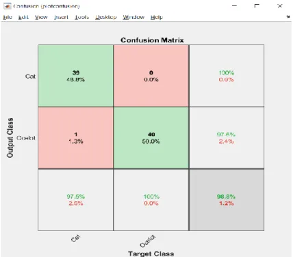
Figure 12 shows the results of using 200 images of each animal, 20% validation set, and 80% training data. It detected that cat is a cat 39 times of 40 and misclassified of detecting the cat one time. For the ocelot, there was no misclassification at all. We can also see that the accuracy has increased by 1,3 % by adding more images.

Figure 12. Results from AlexNet with using 200 images of each animal, training-validation set to 80/20.

(30)

By increasing the validation set to 30%, 60 images will be used for each animal to increase the error rate. So, we will have 30% validation set and 70% training data.

Figure 13 shows the error rate increased by having it misclassified ocelot for a cat two times out of 60 and misclassified cat for ocelot two times out of 60.

Figure 13. Results from AlexNet with using 200 images each animal, and by using 30 % instead of 20 % in the validation set

Figure 13 shows that the pre-trained network misclassified two ocelots for a cat and two cats for an ocelot. Figure 14 shows a misclassification between a cat and an ocelot, where it classified the ocelot for a cat, unlike figure 14, where it correctly classified the ocelot for an ocelot. Where figure 15 shows the correct classification of an ocelot.

(31)

Figure 14. Image that the network misclassified an ocelot for a cat.

(32)

6.2. Training from scratch

The same size of images is used for this network. This network's training is different from the one before, wherein this one, we specify the training options and defines the convolutional neural network architecture. It is almost the same principle for the first experiments. We start by downloading the images in imds. Then we define the convolutional neural network architecture by specifying the size of the images in the input layer and the number of classes in the fully connected layer. The next step after defining the CNN architecture is to train the network and specify the training options. The last step is the same as the first experiment. There the confusion matrix is going to be used after the classification of the validation set.

Figure 16 shows much more misclassification than the pre-trained network and has less accuracy. For this test, we used 20% validation set and 80% training data. It has misclassified a cat for an ocelot 16 times out of 40 and misclassified an ocelot for a cat 14 times out of 40.

Figure 16. Results from trained network from scratch by using 200 images each animal, training-validation set to 80/20.

(33)

Figure 17Results from the trained network from scratch by with using 200 images each animal, and by 30 % instead of 20 % in the validation set.

In figure 17, you can see the result by using 60 images instead of 40. The accuracy has increased to 65,8 %, but it also misclassified more images. The same image as in figure 14 was correctly classified, were in figure 14 it misclassified an ocelot for a cat, but here we got the same image but correct classified—figure 18, where it misclassified an ocelot for a cat.

(34)

6.3. ResNet-18

It is almost the same in the third and first experiments, except we use another pre-trained network instead of the one we had in the first experiment. ResNet-18 will be used as a trained network. This experiment is almost the same as AlexNet but in this experiment the pre-trained network requires input images of size 224-by-224-by-3 instead of 227-by-227-by, and we going to resize all the image by creating augmented image datastore. This part of the code will resize all the images that we have from 227x227x3 to 224x224x3.

augimdsTrain = augmentedImageDatastore(inputSize(1:2),imdsTrain); augimdsTest = augmentedImageDatastore(inputSize(1:2),imdsTest);

As shown in figure 19, by using 70 % training and 30 % test data, it misclassified 1 ocelot for a cat. The error rate is too small unlike the other pre-trained network AlexNet where we got so little error rate by using 80 % training and 30 % test data.

Figure 19. Result by using ResNet-18 with using 200 images each animal, and 70% training and 30% test data

Figure 20 shows the only image that was misclassified for a cat, but it is an ocelot, and this image was classified correctly in some of the tests that we did in the previous networks.

(35)

Figure 20. Misclassified image by ResNet of an ocelot for a cat.

We tried to do the same thing as for the AlexNet for ResNet-18 by increasing the error rate by increasing the training and test data shown in figure 21, from 70 % to 60% training data and 30 % to 40 % test data. The error rate increased by having it misclassified ocelot for a cat two times. After increasing the error rate, we got the same misclassified image as in figure 20. So, it misclassified the same image twice.

(36)

6.4. Table of the combined networks

Table 1 shows the results that we get from combining the networks. We used the same training and validation set for all the networks. Net1, Net2 and Net3 will have 70% in the training data and 30 % in the validation set. First, we separated the images, so we have 140 images in training set and 60 images in validation set, then we validated the 60 images. The three networks validate the same 60 images.

Net1: is the first network which is the pretrained AlexNet Net2: network which is trained from scratch

Net3: is the last network ResNet (pre-trained as well)

By combining Net1 and Net2, we got 3 images that were misclassified by the two networks and 22 images that the network made a different classification on. For the second combination we combined Net1 and Net3. We got one image that was misclassified by the two networks and 2 images that the networks made a different classification on. In The third combination Net2 and Net3, we got one image misclassified by the two networks and 20 images that the networks made a different classification on. Interesting to note is that each combination of two networks misclassified different images.

The first alternative was to combine two networks together that is similar to a COM-MON architecture, where both networks need to classify the same image identically for the system to output a result. Otherwise, a fault detected/image mismatch will be sent out. Triple Modular Redundancy (TMR) were used to combine all the three networks together by a voter. As can be seen in table 1, by using TMR we got worse results than by using any COM-MON combination of two networks (which was expected since each combination of two networks misclassified different images).

Networks Same images that are

misclassified by the networks leading to a

misclassified output

Cases where the networks made a different classification, which do not lead to incorrect output but instead signals fault detected

Net1 + Net2 3 22

Net1 + Net3 1 2

Net2 + Net3 1 20

Net1 + Net2 + Net3 5 24

Table 1. results by combining all Networks

Using TMR assumes the failure rates to be similar (and small) in the three networks. If one of the networks has a much higher failure rate than the others, the resulting failure rate will become higher than any of the individual COM-MON par. When combining all networks, five images were misclassified. The three networks did not come to the same conclusion

(cat/ocelot) for 24 images. However, if two networks select ocelot (or cat) they win over the last network with opposite animal. When this happen, no fault detected appears. Fault

detected may however appear if one or more of the networks do not detect the object at all or if one (or more) of the networks identifies another object (other than cat or ocelot), and the others do not agree, i.e. identify one cat and one ocelot.