CESIS Electronic Working Paper Series
Paper No. 457
The Geography of Economic Segregation
Richard Florida Charlotta Mellander
June, 2017
The Royal Institute of technology Centre of Excellence for Science and Innovation Studies (CESIS)
The Geography of Economic Segregation
Richard Florida & Charlotta Mellander* June 2017
Abstract: This study examines the geography of economic segregation in America. Most studies
of economic segregation focus on income, but our research develops a new measure of overall economic segregation spanning income, educational, and occupational segregation which we use to examine the economic, social and demographic factors which are associated with economic segregation across US metros. Adding in the two other dimensions of educational and
occupational segregation– seems to provide additional, stronger findings with regard to the factors that are associated with economic segregation broadly. Our findings suggest that several key factors are associated with economic segregation. Across the board, economic segregation is associated with larger, denser, more affluent, and more knowledge based metros. Economic segregation is related to race and to income inequality.
Keywords: Economic Segregation, Income Inequality, Education, Occupation, Race JEL: R23, I3, J1
*corresponding author
Richard Florida is University Professor and Director of Cities at the Martin Prosperity Institute in the University of Toronto’s Rotman School of Management and Global Research Professor at
NYU, florida@rotman.utoronto.ca. Charlotta Mellander is Professor of Economics at the
Introduction
There has been a surge in interest in inequality among scholars, policy-makers, and the general public over the past decade or so. A large number of studies have documented the sharp
rise in the inequality of nations over the past several decades (Atkinson, 1975, 2015; Card and
DiNardo, 2002; Stiglitz, 2013; Piketty, 2014). Other studies have documented the worsening geography of inequality across U.S. metros (Glaeser et al., 2009; Baum-Snow and Pavan, 2013; Florida and Mellander, 2014).
But, there is also a substantial and growing literature on economic segregation (Logan et al., 2004; Watson et al. 2006; Watson, 2009; Bishop, 2009; Reardon and Bischoff, 2011; Fry and Taylor, 2012; Bischoff and Reardon, 2014). Fry and Taylor (2012) found that the segregation of upper- and lower-income households had risen in 27 of America’s 30 largest metros. The
segregation of the rich and poor rose in all but three of America’s 30 largest metros between 1980 and 2010. Watson (2009) found that approximately 85 percent of people in America’s cities and metro areas live in areas that are more economically segregated today than they were in 1970. Bischoff and Reardon (2014) found that the share of families living in middle class neighborhoods declined from nearly two thirds (65 percent) in 1970 to less than half (44 percent) by 2007. The share of families living in affluent neighborhoods increased from 7 percent to 14 percent and the share of families living in poor neighborhoods rose from 8 to 17 percent. The share of people living in either poor or wealthy neighborhoods doubled over those three-plus decades, from 15 to 31 percent.
Our research examines the geography of economic segregation in America. Most studies of economic segregation focus on income (Watson et al., 2006; Watson, 2009; Reardon and Bischoff, 2011; Fry and Taylor, 2012). But sociologists have long noted the intersection and
interplay of three factors in the shaping of socio-economic status and class position: income, education, and occupation (Wright, 1985, 1997; Weeden and Grunsky, 2005; Lareau and Conley, 2008). Our analysis of economic segregation focuses on all three of these dimensions: income, educational, and occupational segregation. We introduce seven individual and combined measures of income, educational and occupational segregation, and an Overall Economic Segregation Index. The individual indexes are based on the Index of Dissimilarity (Duncan and Duncan, 1955; Massey and Denton, 1988), which compares the spatial distribution of a selected group of people with all others in that location, and they are calculated across the more than
70,000 census tracts that make up America’s 350-plus metros.In addition, it examines the key
economic, social, and demographic factors that are associated with these various types of economic segregation.
The rest of this article is organized as follows. The next section presents our variables, data and methodology. We follow that with a comparison of the different types of economic segregation to identify their inter-relationships and describe the types that appear to be more or less severe. We then present the findings of a correlation analysis which examines the key economic, social, and demographic factors that bear on economic segregation. The concluding section summarizes our key findings and discusses their implications.
Variables, Data, and Methodology
This section presents our variables, data, and methodology. The data cover the more than 70,000 U.S. tracts across all 359 U.S. metropolitan regions.
Economic Segregation Measures
Our key measures of economic segregation are as follows:
Income Segregation
Segregation of the Poor: This covers households below the poverty level in 2010 as defined by
the Census in 2010.
Segregation of the Wealthy: This covers households with an income above $200,000, the highest
income group reported by tract by the Census in 2010.
Income Segregation: This combines the two measures above into a single index. All data are
from the 2010 U.S. Census (2011).
Educational Segregation
Segregation of Non-High School Grads: This measures the residential segregation of adults with
less than a high school degree.
Segregation of College Grads: This measures the segregation of adults with a college degree or
more.
Educational Segregation: This combines the two educational measures into a single index. All
data are from the 2010 U.S. Census.
Occupational Segregation
Creative Class Segregation: This measures the residential segregation of the creative class. Service Class Segregation: This measures the residential segregation of individuals who hold
Working Class Segregation: This measures the residential segregation of the blue collar working
class.
Occupational Segregation: This is an index of the three occupational segregation measures
above. All data are from the 2010 American Community Survey (ACS).
Overall Economic Segregation Index: This index combines the rank of the seven income,
education, and occupation measures into an index of overall economic segregation.
The seven individual indexes are all calculated based on the Index of Dissimilarity (Duncan and Duncan, 1955; Massey and Denton, 1988). It compares the distribution of a selected group of people with all others in that location. The more evenly distributed a group is compared to the rest of the population, the lower the level of segregation. This Dissimilarity Index ranges from 0 to 1, where 0 reflects no segregation and 1 reflects complete segregation. The Dissimilarity Index, D, can be expressed as:
𝐷 = 1 2∑ | 𝑥𝑖 𝑋− 𝑦𝑖 𝑌| 𝑛 𝑖=1
where xi is the number of individuals in our selected group in tract i, X is the number of the
selected group in the metropolitan area, yi is the number of “others” in the Census tract, and Y is the corresponding number in the metropolitan area. n is the number of Census tracts in the metropolitan area. D gives a value to the degree to which our selected group is differently distributed across Census tracts within the metropolitan area, compared to all others. D ranges from 0 to 1, where 0 denotes minimum spatial segregation and 1 the maximum segregation. The more evenly distributed a group is compared to the rest of the population, the lower the level of
segregation.
The combined measures of income segregation, educational segregation, and occupational segregation as well as the Overall Economic Segregation Index are created by combining rankings on each of these individual indexes. Thus, we can no longer interpret the index value as 0 equal to no segregation and 1 equal to complete segregation. These combined index values create a relative measure where the highest index value indicates the most
segregated metro.
Economic, Social, and Demographic Variables
We also examine the relationships between economic segregation and the following demographic, economic, and social variables:
Population Size: Metro population based on 2010 ACS, a. logged version of this variable is used
for the correlation analysis.
Density: Based on population-weighted density measured as distance from the city center or city
hall. This data is from the United States Census and is for the year 2010.
Income: Average income per capita from the 2010 American Community Survey.
Wages: Average metro wage level from the United States Bureau of Labor Statistics (BLS) for
the year 2010.
College Grads: The share of adults with a college degree or more, from the 2010 ACS.
Knowledge/Creative Class: The share of employment in knowledge, professional and creative
occupations including: computer science and mathematics; architecture; engineering; life, physical, and social sciences; education, training, and library science; arts and design work; entertainment, sports, and media; and professional and knowledge work occupations in
management, business and finance, law, sales management, healthcare, and education. This is based on 2010 data from the BLS.
Service Class: The share of employment in low-skill, low-wage service class jobs including:
food preparation and food-service-related occupations, building and grounds cleaning and maintenance, personal care and service, low-end sales, office and administrative support, community and social services, and protective services, also based on 2010 BLS data.
Working Class: The share of employment in blue-collar occupations including: production
occupations, construction and extraction, installation, maintenance and repair, transportation, and material moving occupations. This is also based on 2010 data from the BLS.
Housing Costs: The median monthly housing costs from the 2010 ACS.
Drive to Work Alone: The share of commuters that drive to work alone, a proxy for sprawl, also
from the 2010 ACS.
Take Transit: The share of commuters that use public transportation to get to work, from the
2010 ACS.
Race: We measure four major racial groups per the 2010 ACS: the share of population that is
White, Black, Asian, and Hispanic-Latino.
Gay Index: A location quotient for the concentration of gay and lesbian households, from the
ACS for the years 2005–2009.
Foreign-Born: The percentage of population that is foreign-born, from the 2010 ACS.
Income inequality is based on the conventional Gini Coefficient measure and is from the 2010
Key Findings
We now turn to the connections between these various types of segregation. To what degree are income, educational, and occupational segregation related to, or different from, one another? To get at this, Table 1 summarizes the correlations among the various types of economic segregation expressed as indices of dissimilarity.
[Table 1 about here]
Table 1: Correlations for the Various Segregation Indexes
Income Segregation Educational Segregation Occupational Segregation Overall Economic Segregation Income Segregation 1 0.68** 0.65** 0.83** Educational Segregation 0.68** 1 0.85** 0.94** Occupational Segregation 0.65** 0.85** 1 0.95** Overall Economic Segregation 0.83** 0.94** 0.95** 1
** significant at the 1 percent level.
The specific correlations range from 0.65 to 0.95. When a metro is segregated on one measure, it is likely to be segregated on the others as well. While some metros rank higher and some lower on individual types of economic segregation, the troubling reality is that segregation is all of a piece.
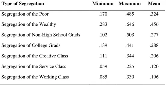
We know that the various types of segregation are related. But are some types more severe than others? To get at this, we examined how segregated the average or “mean” metro is for each of the seven measures. We also looked at the range of segregation across metros, charting the lowest and highest levels of segregation for each segregation measure. Table 2 compares the segregation scores for the average metro as well as the values for the most and least segregated metros for each of our segregation measures. Smaller values reflect lower levels
[Insert Table 2 about here]
Table 2: Scores for Different Sorts of Economic Segregation
Type of Segregation Minimum Maximum Mean
Segregation of the Poor .170 .485 .324
Segregation of the Wealthy .283 .646 .456
Segregation of Non-High School Grads .102 .503 .277 Segregation of College Grads .139 .441 .288 Segregation of the Creative Class .111 .344 .206 Segregation of the Service Class .059 .225 .120 Segregation of the Working Class .085 .330 .196
Of the three types of economic segregation, occupational segregation appears to be the least severe according to these measures. The segregation of the creative class is on average slightly higher (0.206) than that of the working class (0.196). The segregation of the service class is quite a bit lower (0.120). This likely reflects the fact that the service class makes up nearly half of all occupations across the United States and is therefore more evenly spread out
geographically across tracts within metros. Educational segregation occupies the middle ground between income and occupational segregation. The mean values for the less educated (adults who did not complete high school) and the highly educated (college grads) are quite similar (0.277 and 0.288 respectively). That said, the range for less educated groups is greater, indicating a broader range of segregation, even though the means are similar. The segregation of poverty has a mean value of 0.323, higher than any type of occupational or educational segregation. But the most severe form of segregation by far is the segregation of the wealthy, with a mean value of 0.456.
In each case—for income, educational, and occupational segregation—the mean scores for more advantaged groups are higher than for less advantaged groups. This is so for occupational
segregation, where the creative class has a higher mean segregation score than either the working class or service class; for educational segregation, where college grads have a slightly higher mean segregation score than those who did not graduate from high school; and it is especially true for income segregation, where wealth segregation has a much higher score than poverty segregation.
Correlation Analysis Findings
We now turn to the underlying factors and characteristics of metros that are associated with higher or lower levels of overall economic segregation. Table 3 summarizes the key
findings of the correlation analysis for our overall economic segregation index and our measures of income, educational and occupational segregation. (The appendix includes correlations for all economic segregation measures).
[Table 3 about here]
Table 3: Correlation Analysis Findings
Overall Economic \S Sseg SSegregatio n Income Segregation Educational Segregation Occupational Segregation Population Size ..643** .525** .621** .596** Population Density .560** .438** .557** .520** Income .291** .159** .279** .321** Wages .456** .249** .474** .477** College Grads .465** .300** .431** .495**
Service Class -.124* -.109* -.162** -.079
Working Class -.370** -.175** -.354** -.426**
Housing Cost .312** .100 .362** .342**
Drive to Work Alone -.217 .056 -.256** -.314**
Take Transit .377** .232** .337** .417** White -.434** -.254** -.479** -.424** Black .292** .304** .234** .264** Asian .304** .094 .317** .362** Hispanic-Latino .244** .018 .380** .236** Gay Index .422** .067 .478** .514** Foreign-Born .380** .073 .479** .421** Income Inequality .517** .322** .514** .532**
Size and Density: Economic segregation is closely associated with the size and density of
metros. The correlations for population range from 0.525 to 0.643. The correlations for density range from 0.438 to 0.560. Economic segregation thus appears to be a feature of larger, denser metros. The metros with the lowest levels of overall economic segregation are mainly smaller and medium-sized ones. There are more than 200 small and medium-sized metros where overall segregation is less than in the least segregated of the 51 large metros. All 10 of the least
segregated metros in the country have 300,000 people or less.
Income and Wages: Economic segregation is positively associated with income and wager, two
measures of the wealth and affluence of metros. The correlations for income per capita range from 0.159 to 0.321. The correlations for average wage levels range from 0.259 to 0.477.
Education/College Grads: Economic segregation is closely with educational attainment of
metros measured as the percent of adults that are college grads. The correlations here range from 0.300 to 0.495.
Work/Occupational Class: We next look at the correlations to the type of work people do,
measured by three major occupational groups: highly skilled and highly paid workers that make up the knowledge, professional and creative class; the members of the blue-collar working class; and the less-skilled, lower paid members of the service class. Economic segregation is positively associated with the knowledge-creative class. The correlations here range from 0.352 to 0.554). Conversely, we find that economic segregation is negatively associated with the share of workers in blue-collar working-class occupations. The correlations range from -0.175 to -0.426). Having a larger working class appears to militate against economic segregation. The correlations for service class shares are negative and weakly significant in most of the cases, ranging from -0.079 to -0.162.
Housing Costs: Economic segregation is mainly positively associated with higher housing
costs. Most of the correlations are in the mid-3s. But the income segregation correlation is insignificant. Here, we note that we are looking at median values, which do not capture the distribution of housing costs within a metro. A metro with little variation in costs for housing can end up with the same median value for housing as a metro where the variation ranges from very cheap to very expensive. Also, our analysis covers all 350-plus American. metros. Housing costs in high-cost metros like New York or San Francisco likely play a much larger role in residential segregation than they do on average.
Commuting Type: Economic segregation is also related to the way people in different metros
commute to work, namely whether they take transit or drive a car to work. Economic segregation is positively associated with the share of commuters who take transit to work, with correlations in the range 0.322 to 0.417). On the flip side, economic segregation is mainly negatively associated with the share of commuters that drive to work alone. Most of the correlations are in the negative 2s and 3s, but the correlation to income segregation is insignificant. These findings likely reflect the broader effects of size and density. Transit is associated with larger, denser regions; commuters are more likely to drive to work alone in smaller and more sprawling metros.
Race/ Ethnicity: A broad body of research documents the connection between race, poverty,
and segregation (Wilson, 2012; Sampson, 2012; Sharkey, 2013). Our findings indicate that race is connected to economic segregation. Economic segregation is positively associated with the share of adults that are Black. The correlations here range from 0.234 to 0.304. Economic segregation is also mainly positively associated with the share of population that is Hispanic-Latino. The correlations are mainly in the high 2s and 3s, but the correlation for income
segregation is insignificant. Economic segregation is also positively associated with the share of population that is Asian. The correlations here are mainly in the 3s, but the correlation to income segregation is again insignificant. Conversely, economic segregation is negatively associated with the share of the population that is White with correlations ranging from -0.254 to -0.479. Generally speaking, race plays a relatively larger role in educational and occupational
segregation than in income segregation. Generally speaking, the strength of the correlations seem to suggest that the white share of the population plays a relatively greater role in economic segregation than the shares of racial and ethnic minorities.
Diversity: Our analysis shows that economic segregation is positively associated with two
common measures of diversity: the concentration of gay and lesbian people and the share of the population that is foreign-born. Both measures are positively related to all types of economic segregation but income segregation with coefficients around 0.4 to 0.5. More diverse metros tend to be more economically segregated. A 2015 analysis (Silver, 2015) found a relationship between ethnic and racial diversity at the city and neighborhood level. Across the 100 largest cities in the US, those that had higher levels of racial and ethnic diversity overall were found to have the highest levels of racial and ethnic segregation at the neighborhood level.
Inequality: Economic segregation is connected to income inequality (measured by the Gini
coefficient). Three of the correlations are in the 5s, with the correlation to income segregation a bit weaker, 0.322. While income inequality and residential segregation do go together, it is important to remember that they are not the same thing. As Bischoff and Reardon (2014, p. 18) note, “although income inequality is a necessary condition for income segregation, it is not sufficient.” A metro might be quite unequal but not particularly segregated if lower and upper income groups are distributed evenly across neighborhoods. Likewise, a metro could be highly segregated but relatively equal if its different economic groups reside in different neighborhoods.
Conclusion
Our research has mapped measures of economic segregation spanning income, education, and occupation; developed an overall index of economic segregation which combines all three; and examined the key factors associated with economic segregation across American metros. It
informs several key findings.
The most novel contribution of our research seems to be the addition of measures of educational and occupational segregation to the more typical measure of income segregation. The measure of income segregation generates many of the weakest associations in our analysis, in a number of instances the results are statistically insignificant. In particular, income
segregation is less associated with income and wages, educational levels, commuting styles, and racial patterns. Adding in the two other dimensions of educational and occupational segregation consistently generate stronger associations across all of these variables and aspects of our economic and social geography. If anything, it appears that educational and occupational segregation are more serious dimensions of segregation than income segregation. In fact, that would seem to capture dimensions of our locational sorting that are intuitive, as education and the kind of work people do appear to be key factors in people sort into different neighborhoods and areas of the city.
That said, all three types of economic segregation – income, educational and occupational segregation—are associated with one another. If a metro is segregated on one dimension, it increases the likelihood that it is segregated on the others.
In addition, our findings suggest that economic segregation appears to be conditioned by more advantaged groups. The members of the knowledge, professional and creative class is more segregated than either the working or service classes. College graduates are more segregated than those who did not finish high school. Even more so, the wealthy are more segregated than the poor—indeed they are the most segregated of all and by a considerable margin. These more advantaged groups have the resources to isolate themselves from less advantaged groups. This finding is in line with other research on the subject. Fry and Taylor (2012) found that the
population of high-income residents living in high-income neighborhoods or tracts doubled between 1980 and 2010 compared to the population of income households living in low-income neighborhoods, which grew by just 5 percentage points over the same period. Bischoff and Reardon (2014, p. 33) note that the segregation and isolation of the rich has become “consistently greater” than the segregation of the poor over the past several decades.
Generally speaking, our analysis appears to suggest that similar underlying economic and demographic factors are associated with each of the major types of segregation and with
economic segregation overall and especially with educational and occupational segregation. Across the board, economic segregation is also associated with larger, denser, more affluent, and more knowledge based metros.
Furthermore, economic segregation is related to race. It is positively associated with the share of the population that is Black, Hispanic-Latino, or Asian, and negatively associated with the share that is White. And it also appears from our analysis that the strongest relation between race and economic segregation is for the White share of the population. Once again, the
connection between economic segregation and race appears more robust when we include measures of educational and occupational segregation as compared to the variable for income segregation.
Our analysis also finds economic segregation is closely connected to income inequality. Indeed, other research suggests that economic segregation and inequality tend to compound and exacerbate each other. This is in line with other research which notes the negative impacts of economic segregation. Chetty et al. (2014a, 2014b, 2016) find that economic segregation us negatively associated with the ability of children from low-income to move up the economic ladder. Sharkey (2013) finds economic and racial segregation combine to trap those
lower-income and less advantaged Black Americans in neighborhoods of concentrated poverty and distress, leaving them virtually “stuck in place,” with little prospects for upward economic mobility. Diamond (2016) has shown that high-skill, high-pay workers derive additional
advantages from living in safer neighborhoods with better schools, better health care, and a wider range of services and amenities. The inequality of overall “well-being” that they enjoy is 20 percent higher than the simple wage gap between college and high school grads can account for. Conversely, less advantaged communities suffer not just from a lack of economic resources, but from related neighborhood effects like higher rates of crime and drop-outs, infant mortality, and chronic disease.
A decade or so ago, Bishop (2009) noted how talented and educated people were
concentrating more in some places than others, a tendency he dubbed “the big sort.” If anything, our findings suggest that this big sort has now grown into an even bigger sort. America’s
metropolitan areas appear to have cleaved into small clusters of economic advantaged defined by greater incomes, higher levels of education, and knowledge and professional occupations, and large spans of relative disadvantage defined by lower income levels, lower levels of education, and lower-paying blue-collar service occupations.
References
Atkinson, A.B. (1975) The Economics of Inequality, Oxford: Clarendon Press.
Atkinson, A.B. (2015) Inequality, Cambridge, MA: Harvard University Press.
Baum-Snow, N., Pavan, R. (2013) “Inequality and City Size,” Review of Economics and
Statistics, 95(5), 1535-1548.
Bishop, B. (2009) The Big Sort: Why the Clustering of Like-Minded America is Tearing Us
Apart, Boston, MA: Houghton Mifflin Harcourt.
Bischoff, K., Reardon, S. F. (2014) Residential Segregation by Income, 1970–2009, New York: Russell Sage Foundation, available at:
http://www.s4.brown.edu/us2010/Data/Report/report10162013.pdf
Card, D., DiNardo, J. E. (2002) “Skill Biased Technological Change and Rising Wage Inequality: Some Problems and Puzzles,” Journal of Labor Economics, 20(4), 733-783
Chetty, R., Hendren, N., Kline, P., Saez, E. (2014a) “Where Is the Land of Opportunity? The Geography of Intergenerational Mobility in the United States,” The Quarterly Journal of
Economics, 129(4), 1553-1623
Chetty, R., Hendren, N., Kline, P., Saez, E., Turner, N. (2014b) “Is the United States Still a Land of Opportunity? Recent Trends in Intergenerational Mobility,” American Economic Review
Papers and Proceedings, 104(5), 141-147
Chetty, R., Hendren, N., Katz, L. (2016) “The Effects of Exposure to Better Neighborhoods on Children: New Evidence from the Moving to Opportunity Experiment,” American Economic
Diamond, R. (2016) “The Determinants and Welfare Implications of US Workers’ Diverging Location Choices by Skill: 1980-2000,” American Economic Review, 106(3), 479-524
Duncan, O. D., Duncan, B. (1955) “A Methodological Analysis of Segregation Indexes,”
American Sociology Review, 29(1), 210-217
Florida, R., Mellander, C. (2014) “The Geography of Inequality: Difference and Determinants of Wage and Income Inequality across U.S. Metros,” Regional Studies, 50(1), 79-92
Glaeser, E., Resseger, M., Tobio, K. (2009) “Inequality in Cities,” Journal of Regional Science, 49(4), 617-646
Lareau, A., Conley, D. (eds) (2008) Social Class: How Does It Work?, New York: Russell Sage Foundation
Logan, J. R., Stults, B. J., Farley, R. (2004) “Segregation of Minorities in the Metropolis: Two Decades of Change,” Demography, 41(1), 1-22
Massey, D. S., Denton, N. A. (1988) “The Dimensions of Residential Segregation,” Social
Forces, 67(2), 281-315
Reardon, S. F., Bischoff, K. (2011) Growth in the Residential Segregation of Families by
Income, 1970–2009, Russell Sage Foundation, available at: http://www.s4.brown.edu/us2010/Data/Report/report111111.pdf
Piketty, T. (2014) Capital in the Twenty-First Century, Cambridge, MA: Belknap Press
Sampson, R. J. (2012) Great American City: Chicago and the Enduring Neighborhood Effect, Chicago, IL: University of Chicago Press
Equality, Chicago, IL: The University of Chicago Press
Silver, N. (2015) “The Most Diverse Cities Are Often the Most Segregated,” FiveThirtyEight, May 1, available at: https://fivethirtyeight.com/features/the-most-diverse-cities-are-often-the-most-segregated/
Stiglitz, J. (2013) The Price of Inequality, New York: W. W. Norton & Company
Fry, R., Taylor, P. (2012) The Rise of Residential Segregation by Income, Washington, D.C.:
Pew Research Center, available at:
http://www.pewsocialtrends.org/files/2012/08/Rise-of-Residential-Income-Segregation-2012.2.pdf
Watson, T., Carlino, G., Gould Ellen, I. (2006) “Metropolitan Growth, Inequality, and Neighborhood Segregation by Income,” Brookings-Wharton Papers on Urban Affairs, 1–52
Watson, T. (2009) “Inequality and the Measurement of Residential Segregation by Income in American Neighborhoods,” Review of Income and Wealth, 55(3), 820–844
Weeden, K. A., Grunsky, D. B. (2005) “The Case for a New Class Map,” American Journal of
Sociology, 111(1), 141–212
Wilson, W. J. (2012) The Truly Disadvantaged: The Inner City, the Underclass, and Public
Policy, Chicago, IL: University of Chicago Press.
Wright, E. Olin (1985) Classes, London: Verso
Wright, E. Olin (1997) Class Counts: Comparative Studies in Class Analysis, Cambridge, MA: Cambridge University Press
Appendix:
Poor Wealthy Non-High
School Grads College Grads Creative Class Service Class Working Class Population Size .427** .377** .575** .538** .603** .282** .614** Density .536** .172** .626** .392** .557** .392** .420** Income .397** -.154** .367** .154** .237** .327** .339** Wages .461** -.079 .536** .343** .479** .413** .444** College Grads .508** -.037 .472** .320** .306** .456** .571** Knowledge/ Creative Class .480** .062 .483** .421** .422** .472** .591** Service Class -.201** .033 .118* -.180** -.152** .034 -.138** Working Class -.207** -.062 -.391** -.253** -.320** -.459** -.345** Housing Cost .291** -.143** .517** .172** .370** .301** .307** Drive to Work Alone -.090 .169** -.349** -.146** -283** -.385** -.276** Take Transit . 367** .014 . 332** .281** .368** .447** .379** White -.102 -.286** -.424** -.445** -.512** -.282** -.315** Black .119* .338** .057 .336** .220** .170** .233** Asian .223** -.067 .359** .237** .371** .355** .329** Hispanic-Latino -.094 .152** .459** .251** .449** .056 .110* Gay Index .104 .001 .515** .388** .518** .416** .461** Foreign-Born .071 .062 .572** .334** .589** .261** .340** Income Inequality .223** .306** .355** .575** .477** .354** .499**