Acoustic Radiation Of An Automotive Component Using Multi-Body Dynamics

(1)

IN

DEGREE PROJECT VEHICLE ENGINEERING, SECOND CYCLE, 30 CREDITS

,

STOCKHOLM SWEDEN 2020

Acoustic Radiation of an

Automotive Component using

Multi-Body Dynamics

(2)

ACOUSTIC RADIATION OF AN AUTOMOTIVE

COMPONENT USING MULTI-BODY DYNAMICS

Vehicle Engineering

Master Thesis

Shayan Aghaei

GKN

KTH Royal Institute of Technology

October 2020

(3)

Acknowledgements

Firstly, I’d like to express my gratitude to Stefano Orzi and Eva Lundberg at GKN for their guidance and support throughout the duration of this thesis. Secondly, I’d like to thank Shivanand Ambalavanan, Rafal Czech and Ravi Bandlamudi for their excellent advice and technical support.

A huge thanks to Ulf Carlsson, my supervisor at KTH, who provided me with excellent insight and guidance. Also, thank you to Lars Drugge for his advice throughout the project.

Finally, but my no means least, thank you to my friends and family for their unwavering support.

(4)

List of Abbreviations

AWD . . . All Wheel Drive BC . . . Boundary Conditions

CAE . . . Computer Aided Engineering CMS . . . Component Mode Synthesis DAE . . . Differential Algebraic Equations DFT . . . Discrete Fourier Transfer

DOF . . . Degrees of Freedom EOL . . . End-of-Life

FEA . . . Finite Element Analysis FSC . . . Fluid Structure Coupling FSI . . . Fluid Structure Interaction MBD . . . Multi-body Dynamics MNF . . . Modal Neutral File

NVH . . . Noise Vibration & Harshness OSWL . . . Overall Sound Power Level PSD . . . Power Structural Density PTU . . . Power Transfer Unit RDU . . . Rear Differential Unit SP(L) . . . Sound Pressure (Level) SW(L) . . . Sound Power (Level) TE . . . Transmission Error TRB . . . Tapered Roller Bearings

(5)

Abstract

An important facet of creating high-quality vehicles is to create components that are quiet and smooth under operation. In reality, however, it is challenging to measure the sound that some automotive components make under load because it requires specialist facilities and equipment which are expensive to acquire. Furthermore, the motors used in testbeds drown out the noise emitted from much quieter components, such as a Power Transfer Unit (PTU). This thesis aims to solve these issues by outlining the steps required to virtually estimate the acoustic radiation of a PTU using the Transmission Error (TE) as the input excitation via multi-body dynamics (MBD). MBD is used to estimate the housing vibrations, which can then be coupled with an acoustic tool to create a radiation analysis. Thus, creating a viable method to measure the acoustic performance without incurring significant expenses. Furthermore, it enables noise and vibration analyses to be incorporated more easily into the design stage.

This thesis analysed the sound radiated due to gear whine which arises due to the TE and occurs at the gear mesh frequency and its multiples. The simulations highlighted that the TE can be accurately predicted using the methods outlined in this thesis. Similarly, the method can reliably obtain the vibrations of the housing. The results from this analysis show that at 2000 rpm the PTU was sensitive to vibrations at 500, 1000 and 1500 Hz, the largest amplitude being at 1000 Hz. Furthermore, the Sound Power Level (SWL) was proportional to the vibration amplitudes in the system. Analytical calculations were conducted to verify the methods and showed a strong correlation. However, it was concluded that experiments are required to further verify the findings in this thesis.

(6)

Sammanfattning

En viktig aspekt i att skapa fordon av hög kvalitet är att skapa komponenter som är tysta och smidiga under drift. I verkligheten är det dock svårt att mäta ljudet som vissa fordonskompo-nenter ger under belastning eftersom det kräver specialanläggningar och utrustning, vilket är dyrt att skaffa. Dessutom maskerar motorerna som används i testbäddar ut bullret från mycket tystare komponenter, till exempel en kraftöverföringsenhet (PTU). Detta examensar-bete syftar till att lösa dessa problem genom att beskriva de steg som krävs för att virtuellt uppskatta den akustiska strålningen av en PTU med hjälp av transmissionsfelet (TE) som ingångsexcitation via flerkroppsdynamik (multi-body dynamics, MBD). MBD används för att uppskatta kåpans vibrationer, som sedan kan kopplas till ett akustiskt verktyg för att skapa en ljudutstrålningsanalys. Således skapas en genomförbar metod för att mäta den akustiska pre-standan utan att medföra betydande kostnader. Dessutom möjliggör det att lättare integrera ljud- och vibrationsanalyser i designfasen.

Detta examensarbete analyserade ljudet som utstrålats på grund av kugghjulsljud, som uppstår på grund av TE och uppträder vid kuggingreppsfrekvensen och dess multiplar. Simuleringarna belyste att TE kan förutsägas exakt med de metoder som beskrivs i detta examensarbete. På samma sätt kan metoden på ett tillförlitligt sätt uppnå kåpans vibrationer. Resultaten från denna analys visar att vid 2000 rpm var PTU känslig för vibrationer vid 500, 1000 och 1500 Hz, den största amplituden var vid 1000 Hz. Dessutom var ljudeffektsnivån (SWL) proportionell mot vibrationsamplituderna i systemet. Analytiska beräkningar genomfördes för att verifiera metoderna och visade en stark korrelation. Dock drogs slutsatsen att experiment krävs för att ytterligare verifiera resultaten i detta arbete.

(7)

1 Introduction

This section gives an insight into the background of this project, the importance of this thesis and the aims.

1.1 Background

Manufacturers within the automotive sector are confronted with the challenge of creating intricate designs of vehicles and their components, which is a highly demanding task as the industry grows to become more competitive. Managing the amount of noise and vibra-tions that radiate throughout the cabin and to by-standers is an important facet of creating innovative and supreme vehicles.

As a consequence of this demand for enhanced ride quality, the Noise, Vibration and Harsh-ness (NVH) behaviour of components must be analysed effectively to identify design areas to improve. This is a key area of development for component manufacturers in the sector, such as GKN Automotive, who are eagerly seeking to develop reliable and accurate methods to predict the NVH characteristics of their parts.

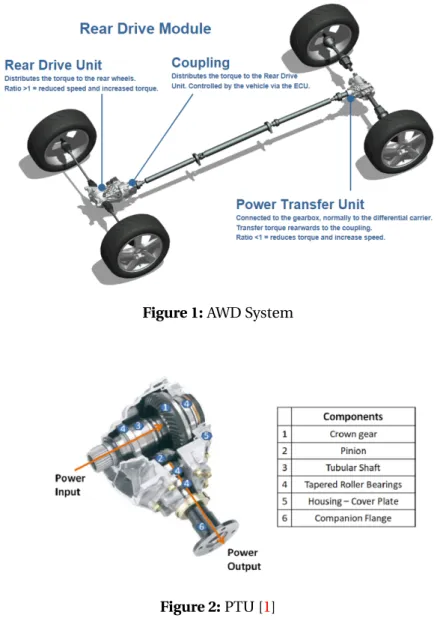
GKN Automotive is one of the world’s largest manufacturer of driveline parts. The plant in Köping (Sweden) is focused on developing and manufacturing driveline systems, particularly all-wheel-drive (AWD) components systems. GKN can provide an AWD system with con-nect/disconnect features for better fuel optimisation. The AWD system consists of a Power Transfer Unit (PTU) and Rear Drive Unit (RDU). The PTU is connected to the gearbox and transfers torque rearwards to the coupling. The RDU distributes the torque to the rear wheels. The layout of this system can be seen in figure1. The PTU and its subcomponents can be seen in more depth in figure2.

(10)

Figure 1: AWD System

Figure 2: PTU [1]

The PTU consists of a hypoid gear set (crown and pinion), the tubular shaft, tapered roller bearings (TRBs), the housing, the cover plate and the companion flange (figure 2). It is widely known that a key contributor to the noise and vibrations in hypoid gears is due to the Transmission Error (TE). Studies in the automotive sector have evidenced that the TE gives rise to significant vibrations and is the fundamental cause of gear whine [2]. In extreme cases, TE can cause vehicles to fail environmental EU regulations on sound pollution and noise control [3].

The human ear is extremely agitated by gear whine due to its tonality. Therefore, it is vital to create virtual models which can use the TE as an excitation source for the acoustic radiation. The virtual model must accurately predict the TE, the noise transfer path and the sound

(11)

heard by the receiver. In the future, these models can help designers improve aspects of the gear design to reduce the TE, thus improving the NVH performance.

1.2 Purpose and Aims

Previous studies on both the PTU and RDU conducted at GKN have shown that reliable virtual models of these components are feasible through various software [4] [5] [1]. These models have demonstrated that it is possible to simulate the dynamic behaviour of these components under load effectively, up to 2000 Hz. More extensive research on the PTU has confirmed that a modal analysis is possible and even the non-linear effects of bearings can be considered. However, previous studies solely focused on structural/vibrational analysis, e.g. a modal analysis, or the TE.

This thesis builds on previous research to create a more robust model of the PTU under dynamic load as well as including the acoustic radiation during operation. The main ob-jectives of this thesis are to estimate the acoustic performance of the PTU by integrating different simulation tools and validating the model. It is necessary to simulate the acoustic radiation virtually because it is difficult to measure the sound in reality due to the motors in the testbeds drowning out any noise made by the PTU. Furthermore, acoustic testing requires expensive equipment and facilities. Therefore, a virtual method of predicting the acoustic radiation would significantly reduce costs and the time to market.

To summarise, the aims of this thesis are:

• Create a Multi-Body Dynamic model of the PTU • Validate the model by using test data

• Create a model which can predict the acoustic radiation • Validate the radiation results

(12)

2 Frame of Reference

This section gives an overview of the knowledge required to understand this thesis.

2.1 Machine Design

2.1.1 Hypoid Gears

The PTU consists of a hypoid gear set, a smaller gear (the pinion) and larger gear (the crown gear). Hypoid gears are a type of bevel gear which are used extensively in the automotive sector to transmit power between perpendicular shafts to the rear axle. A key design benefit of hypoid gears is that the axes are offset. This offset can be either positive or negative, as shown in figure3. Thus, enabling the shaft that drives the pinion to be raised or lowered at the cost of reducing mechanical efficiency.

Figure 3: Offset in Hypoid Gears [6]

2.1.2 Hypoid Gear Contact Ratio

The contact ratio represents the average number of teeth meshing at the same time. The contact ratio refers to ratio of the length of the arc of contact (blue line figure4) to the circular pitch (orange line figure4). The benefit of having a higher contact ratio is that the load is

(13)

shared more equally, resulting in less wear. Furthermore, the average stiffness of the gear is higher. A higher stiffness means better transmission accuracy due to less tooth deflection resulting in a lower TE. Thus, a higher contact ratio results in less noise since TE is the main source of gear noise in driveline parts [7] (see sections2.1.4and2.1.3).

Figure 4: Contact Ratio [7]

2.1.3 Gear Mesh Stiffness and Gear Mesh Frequency

Gear mesh stiffness is a material property of the gear which resists deformation. The value is dependent on the gear material, tooth curvature, tooth loading, contact ratio and angular position of the gear [1]. Since the gear contact and tooth loading changes with time (due to tooth bending), the gear mesh stiffness is dynamic rather than a constant value. This results in a variation of the force acting on the gear teeth, generating a TE and thus causing vibrations. Gear mesh stiffness can be calculated using equation1.

Km=

F el− eo

(1)

where: Km= Gear mesh stiffness

F = Contact force in the line of action

el = translational loaded TE

eo = translational unloaded TE

The gear mesh frequency is the rate at which gear teeth mate together. It can be calculated as shown in equation2. The shaft speed refers to the input shaft when there are multiple

(14)

gears. The number of teeth refers to the pinion, which in this case is 15. This value is important because it has been shown that the gear mesh frequency and its harmonics are the frequencies which contribute heavily to the noise and vibration of gears, particularly gear whine [3] [8]. Table1shows the gear meshing frequencies of the speeds analysed in this thesis.

Gear Mesh Frequency = Nt eet h∗ Rotsha f t (2)

where: Nt eet h = Number of teeth

Rotsha f t= Rotation speed of the shaft (rotations/s)

Table 1: Gear Mesh Frequencies Analysed in this Thesis

Gear Mesh Frequency (Hz)

Speed (rpm) Fundamental First Harmonic Second Harmonic

60 15 30 45

2000 500 1000 1500

2.1.4 Transmission Error

TE is the main excitation source of gear noise during vehicle operation, particularly gear whine [8]. It produces a particularly aggravating noise due to its tonality. TE arises due to gear teeth imperfections during manufacturing and assembly [9]. The imperfections inhibit the gear from transmitting the rotational input correctly, causing a variation in the speed ratio. Consequently, the gear ratio is altered slightly and varies with time. These deviations are the main cause of oscillating forces on the gear teeth, which result in noise and vibrations. The oscillations produced as a result of TE can range between a high or low frequency, depending on the teeth characteristics, such as friction, teeth deflections and geometry.

TE can be defined as ’the difference between the actual position of the output gear and the position it would occupy if the gear drive were perfectly conjugate’ [10]. This is expressed in mathematical terms in equation3and a graphical representation can be observed in figure

5. T E = Θg ear− µ_R pi ni on Rg ear ¶ Θpi ni on (3)

(15)

where: Θg ear = Angular position of the gear Θpi ni on= Angular position of the pinion

Rpi ni on = Pitch circle radius of the pinion

Rg ear = Pitch circle radius of the gear

Figure 5: Transmission Error [5]

2.1.5 Bearings

The PTU contains four TRBs. From figure8in section2.2.5, it is evident that the TRBs must be modelled with a high level of precision as it is important to capture the bearing forces, for noise and vibration analyses. TRBs consist of an outer ring, an inner ring, roller and cage. Figure6below shows the individual parts and their arrangement.

(16)

TRBs are advantageous compared to traditional ball bearings because they reduce friction and in turn, reduce heat generated under operation. The reduced friction and heat dramatically reduce the wear. Hence, TRBs are widely used in automotive applications. Furthermore, the taper enables it to transfer loads evenly whilst rolling when compared to other bearings. Bearings play a crucial role in the NVH behaviour of the PTU as they transmit vibrations from the hypoid gear to the housing (see section2.2.5). Also, they generate dynamic forces and thus sound, due to rolling element contact forces. Previous studies have shown that properties such as the bearing stiffness, bearing damping and bearing position can affect the transmission of excitations [12]. However, modelling bearings is challenging as they exhibit non-linear behaviour which means the stiffness and damping of the bearings change with load and speed [13]. This can be difficult to model and most software solutions attempt to linearise these. In most cases, this is a reasonable simplification. However, a non-linearised solution will yield more accurate results, particularly regarding NVH.

2.2 Noise, Vibration and Harshness

Noise and vibrations are an inevitable by-product of mechanical machines. NVH, in auto-motive applications, is the study of the sounds and vibrations concerning vehicles and their components.

2.2.1 Vibrations - The Fundamentals

Vibration is defined as the periodic back-and-forth motion of particles of an elastic body or an elastic medium. Commonly, this is a result of a physical system being displaced from its equilibrium condition. All bodies containing mass and elasticity are capable of experi-encing vibrations [14]. Thus, most machines and structures engineers deal with experience vibrations to some degree [15].

There are two classes of vibrations:

• Free vibration — A system oscillating due to the forces inherent in a system and no external forces are present. A system that vibrates freely will vibrate at one or more of its natural frequencies.

• Forced vibrations — Vibration that is caused by an external force. If the excitation is oscillatory, the system is forced to vibrate at the excitation frequency.

(17)

• Natural frequency — The frequency at which a system/object oscillates when not subjected to an external force or damping force. All systems and components have at least one natural frequency and it is dependent on its mass and stiffness. Note, sometimes this may be referred to as an eigenfrequency.

• Mode shape — The motion pattern of a system oscillating at a frequency. Commonly bending, torsion or a mixture of the two.

• Resonance — Dangerously large oscillations that occur when a system is excited by a frequency close to its natural frequency. Resonance can be the cause of major structural failure.

• Damping — The energy dissipation due to friction and other resistances. Low damping has only a minor effect on the natural frequency, which is why natural frequency is often calculated without damping. However, high damping can significantly reduce vibration amplitudes.

2.2.2 Acoustics - The Fundamentals

Acoustics is the study of mechanical waves in solids, gases and liquids.

Sound is the oscillation as pressure, stress, particle displacement/velocity is propagated as an acoustic wave through a transmission medium with internal forces, such as a gas, liquid or solid.

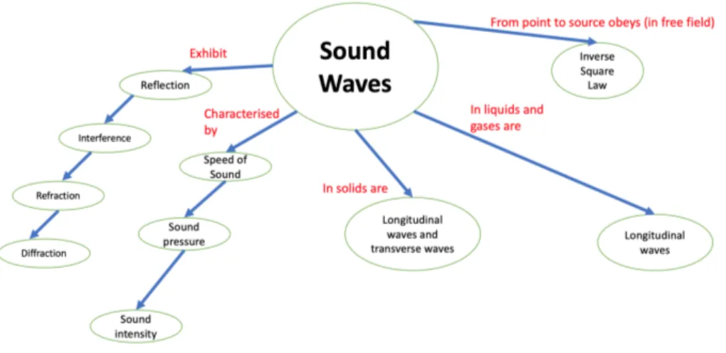
A wave is a disturbance travelling through a medium from one location to another, transport-ing energy. Waves can be reflected, superposed, refracted and diffracted at boundaries, as specified in figure7.

(18)

Figure 7: Basics of Sound Waves

The relationship between the speed of sound, frequency and wavelength is given in equation

4. The wave propagation speeds are generally not dependent on the wave characteristics such as frequency and amplitude. Instead, they are a characteristic of the media in which they travel as observed in equation5, e.g. the speed of sound in air at 20◦C is 340 m/s.

c = f λ (4)

where: c = Speed of sound

f = Frequency λ = Wavelength c = s elastic properties inertial properties= s β ρ (5)

where: β = Bulk modulus

ρ = Density

Sound is usually defined in terms of Sound Pressure (SP) measured in Pa (as observed in figure7) or in its logarithmic form the Sound Pressure Level (SPL). The SPL is measured in decibels (d B ). This is a logarithmic ratio scale (as highlighted in equation6) between the

(19)

measured effective sound pressure (Pr ms) and a reference sound pressure (Pr e f), usually the threshold of hearing, i.e. 20x10−5P a.

SPL (dB) = 20log10 µ Pr ms Pr e f ¶ = 20 log10Pr ms− 20 log10Pr e f (6)

Measuring sound in terms of SP is advantageous because it can be measured directly using a microphone and it will be similar to what the human ear will hear when using a special weighting formula. On the other hand, a drawback of measuring sound in terms of SP is that it is highly dependent on the surrounding environment. The sound you hear will change depending on your distance from the source, whether there are walls or floors which will reflect or absorb the sound. Therefore, it is difficult to draw a direct comparison between two independent results as they are situationally dependent. Instead, one can quantify sound in terms of Sound Power (SW) or its logarithmic version the Sound Power Level (SWL).

SW is the rate acoustic energy is emitted by a source. The difference between SP and SW can be exemplified by considering the difference between the power and temperature produced by a heater. If you stand close to the heater, the temperature will feel much higher than if you stand further away from the heater. Thus, it may be said that the temperature that you feel, similar to the sound pressure you hear, depends on your distance from the heater (or sound source) and the environment you are in, e.g. whether you are in a small room or large room. However, the power consumed by the heater will stay the same regardless of the environment. Power is measured in Watts (W). However, for acoustic purposes, SWL can be measured in dB, relative to a reference power (Wr e f) of 10−12W . Equation7shows SWL in terms of dB.

SWL (dB) = 10log10 µ W Wr e f ¶ (7)

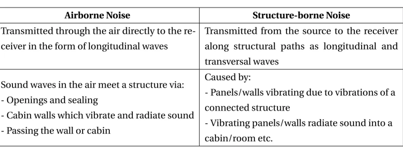
2.2.3 Airborne and Structure-Borne Noise

Acoustic phenomena occur in three different forms, structure-borne noise, airborne noise or a combination of the two. These relate to the medium (transfer path/mechanisms), through which they radiate. A comparison between structure-borne noise and airborne noise can be found in table2.

(20)

Table 2: Comparison of Structure-borne and Airborne Noise

Airborne Noise Structure-borne Noise

Transmitted through the air directly to the re-ceiver in the form of longitudinal waves

Transmitted from the source to the receiver along structural paths as longitudinal and transversal waves

Sound waves in the air meet a structure via: - Openings and sealing

- Cabin walls which vibrate and radiate sound - Passing the wall or cabin

Caused by:

- Panels/walls vibrating due to vibrations of a connected structure

- Vibrating panels/walls radiate sound into a cabin/room etc.

Fluid-Structure Interaction (FSI), sometimes referred to as Fluid-Structure Coupling (FSC), is the interaction between a structure, e.g. floor, panel or wall and a fluid volume, e.g. room or cabin.

2.2.4 Sound Field Definitions

Sound fields refer to a region largely based on the distance from the acoustic source. The definitions of the free, near, far and direct field can be found below [16]:

Free field is defined as a region in space where sound may propagate free from any form of

obstruction.

Near field is the region close to the source of the sound, where the sound pressure and

acoustic particle velocity are not in-phase. The region’s distance from the source is equal to a wavelength of sound or equal to three times the largest dimension of the sound source, whichever is largest.

Far field is the region which begins where the near field ends and extends to infinity. Note, in

reality, this transition is very gradual. In this region, the sound pressure will generally decay at a rate of 6 dB every time the distance from the source is doubled.

Direct field of a sound source is the region where the sound has not been inhibited by any

(21)

2.2.5 Transfer Path Analysis

Transfer path analysis is a systematic method to understand the relation between multiple sources of noise and vibration and their effect on perceived user comfort and health [17]. The aim is to understand the energy propagation paths between the source and the receiver. The method can be used to evaluate the importance of the contribution of different excitation sources. Figure8highlights the energy transfer path of the PTU.

Figure 8: Transfer Path

The gear excitation is caused by the TE (see section2.1.4) which acts on the internal dynamics of the system resulting in the shaft moving laterally. Consequently, the bearings experience dynamic forces. These forces transfer from the bearings to the housing causing the housing to vibrate, which induces noise [18]. From figure8, it is evident that not every sub-component of the PTU is required to capture the acoustic behaviour, i.e. the flange. Furthermore, a model which can accurately capture the gear excitation (TE) and housing vibrations is necessary to predict the noise radiation.

2.2.6 Computer Aided Engineering Techniques

The task of NVH engineers is to create methods to predict, analyse and reduce the noise and vibration that radiates. Several techniques can be employed to achieve this. For instance, analytically, experimentally or through other means. It is imperative that NVH issues are detected and resolved early in the design phase. Early detection can significantly reduce the number of design iterations, keeping costs low as NVH problems typically require revised

(22)

designs. Late detection, e.g. during the prototype phase, can cause significant increases in the development time and unsatisfactory solutions being implemented [19].

A particularly effective way of predicting and improving the NVH characteristics of compo-nents is through Computer-Aided Engineering (CAE). CAE is ‘the use of computer software to simulate the performance of a product to improve the design or facilitate solving engineering problems’ in various engineering disciplines [20].

Usually CAE consists of the following [20]:

1. Pre-processing — model the geometry and assign physical properties (e.g. by applying loads and constraints).

2. Solving — model is solved using the appropriate mathematical and physical con-cepts/formulas.

3. Post-processing – Review of the results and further analysis.

As a result of the improving computational power, NVH engineers now have the means to utilise both Multi-Body Dynamic (MBD) simulations and Finite Element Analysis (FEA) techniques in conjunction with acoustic tools. These simulation techniques enable one to predict the vibrational and acoustic behaviour of parts to a high degree of reliability if the models can capture the important physics at play. The key benefit of using CAE techniques for analysis is that no prototypes are needed, cutting vast amounts of time and costs. Furthermore, problem areas can be detected early in the design phase which, as previously mentioned, is paramount to rectifying NVH issues. As a result, CAE techniques are widely used to solve NVH problems.

Despite substantial yearly improvements in computational power, very large models which contain many elements still require significant resources when solving complex engineering problems. Simplifications must be made to these models which can reduce computation time for more information see section2.3.1and2.3.3. Sometimes, the simplifications are made at the expense of their accuracy. Moreover, no model can fully capture reality meaning that some effects may be unaccounted for. Consequently, results obtained via CAE should be validated with experimental tests.

(23)

2.3 Finite Element Analysis

2.3.1 Component Mode Synthesis

Component Mode Synthesis (CMS) is a modal coupling technique used to describe compo-nents by their modal displacement, coupled together (synthesis) via their common bound-aries to perform a dynamic analysis [21]. In other words, components are subdivided into their substructures and are analysed independently to obtain natural frequencies and mode shapes. Then, by applying boundary conditions, the modal participation, a measure of how strongly a given mode contributes to the response of a structure, can be determined [22]. This technique is advantageous because it significantly reduces the Degrees of Freedom (DOF) of a system, reducing the computational time.

2.3.2 Modal Superposition

Modal superposition may be applied to both free and forced vibration cases. This method uses the free vibration mode shapes to uncouple the equations of motions, which become the modal coordinates. Solutions for the modal coordinates are obtained by solving each equation of motion separately. Then, a superposition of the modal coordinates gives the solution of the original equations. Figure9displays the method of modal superposition, i.e. how the left-hand side is created by adding the contributions of these loads.

Figure 9: Modal Superposition

2.3.3 Craig Bampton Analysis

A common CMS technique is the Craig-Bampton method. The Craig-Bampton method allows users to select a subset of DOF which will not undergo modal superposition [23]. The DOF are selected at specific nodes where attachments are placed. These nodes become interface nodes after completion. This enables users to fully capture the effects of attachments on

(24)

bodies as these are preserved with no loss of resolution regardless of the frequency.

To conduct a Craig-Bampton analysis, the FE model is divided into boundary DOF and interior DOF and solved for two sets of modes, constraint modes and fixed boundary modes, where:

• Constraint modes — Modes obtained when each boundary DOF is given a unit displace-ment whilst simultaneously fixing all other DOF [1][24]. This represents the external mating features. Constraint modes can be observed in figure10.

Figure 10: Constraint Modes [1]

• Fixed boundary normal modes — Boundary DOF are fixed and modes are calculated by deducing the eigen-value solution. These modes represent the internal dynamic properties of the body [1][24]. Fixed boundary normal modes can be found in figure11.

Figure 11: Fixed Boundary Modes [1]

2.4 Acoustic Simulations

Generally, it is difficult to conclusively predict the acoustic radiation of moving bodies, such as transmissions and gearboxes, due to the interaction between subcomponents which causes vibrations and fluctuations in contact forces. These fluctuations are difficult to capture accurately, and consequently, the traditional modelling process is extremely time-consuming.

(25)

Conventionally, acoustic simulations are conducted in three main steps, as exhibited in figure

12. Firstly, an MBD simulation is created to calculate the loads on the structure. Next, an FE analysis is conducted to calculate the vibration of the structure from the applied loads. Finally, the acoustic simulation is solved by using the vibration Boundary Conditions (BC) obtained through the FE analysis.

Figure 12: Conventional Method To Conducting Acoustic Simulations

The conventional method is robust. However, the compatibility between the different soft-ware is not always seamless. For example, an MBD simulation is usually conducted in the time-domain, but this cannot be directly exported to the acoustic tool. Hence, a conversion is required to convert the structure’s response to the frequency-domain, only then can the acous-tic software read the surface vibrations. As a result, this method is incredibly time-consuming and laborious.

Recent advancements in this area has given rise to the capability of directly coupling MBD software with the acoustic software through the use of a plugin. The main benefits of using such a plugin is that all processes are automated, meaning that all results are calculated in the MBD interface. This automation significantly reduces the effort, time and costs required to get reliable acoustic data which will help NVH engineers shorten the design phase of products. The newer process can be seen in figure13.

(26)

The Adams2Actran plugin can predict the noise radiation by using the vibrations of the flexible body calculated by Adams. The benefit of the plugin is that it creates the acoustic meshes automatically without leaving the Adams interface. Instead, Actran runs in the background. First, the program creates an exterior 2D mesh, generally referred to as the shrink wrap but may also be called the boundary condition mesh, around the outer face of the vibrating body. A 3D mesh is created around the shrink wrap, which is called the finite fluid volume. A non-reflective boundary condition is added to the outer face of the finite fluid volume to represent the propagation in the air. Actran achieves the non-reflective boundary conditions by implementing infinite elements on the outer face of the 3D mesh, which also enables pressure values to be computed outside of the fluid volume.

The velocity field of the radiating structure is computed by Adams and projected onto Actran’s shrink wrap (BC mesh). This is used as a velocity boundary condition and is propagated by Actran in the infinite field. The acoustic analysis can be conducted in either the time domain or frequency domain. In both cases, a direct solver is used.

There are two coupling methods between a vibrating structure and the surrounding air, one-way coupling and two-one-way coupling. Two-one-way coupling is when vibrations induce noise and noise induces vibration. Conversely, one-way coupling only considers noise induced by vibrations. Figure14illustrates the difference between one-way and two-way coupling. Two-way coupling is more commonly used in cases where the fluid is water, e.g. submarine analyses. Generally, one-way coupling is sufficient for the radiation in air and is the coupling method used in this thesis.

(a) One-way Coupling (b) Two-way Coupling

(27)

3 Methodology

This section provides information on the methodology used to produce the virtual model of the PTU and how to conduct the simulations.

3.1 Overview

Initially, a transfer path analysis was conducted to gain an understanding of the physics involved and how the components interact with each other to produce the noise. Moreover, the transfer path analysis determined which components were required to be modelled and which components required more detail. As mentioned in section2.2.5, the TE excitation and housing vibrations were identified as critical factors which needed to be modelled correctly.

Secondly, a methodology was created to determine the steps required to produce a viable virtual model that can be used by both the acoustic software and the multi-body dynamics software. The methodology was split into three different stages. The first stage was pre-processing, where the components were meshed, and the correct file types were obtained. The second stage was the MBD, where simulations were conducted to capture the correct housing behaviour and TE. Finally, the acoustic simulations were conducted to determine the sound power level and acoustic radiation. Figure15illustrates the methodology.

Figure 15: Overview of the Methodology

From figure16it can be observed that the SimLab software was used to discretise the com-ponents and add connection points to prepare for an FE analysis. The files were exported in the BDF format. More information can be found in section3.2.1. The files were then imported into MSC Marc, and a reduction in the DOF, via a Craig-Bampton analysis, was

(28)

conducted to reduce the computational time and retain the behaviour of attachment points. A job was created to generate the flexible bodies (i.e. MNF files) which contain the modal information of the components, obtained through an eigenfrequency analysis. Please consult section3.2.2for more information. The MNF files were imported into MSC Adams, and the boundary conditions were modelled. Different dynamic loads were simulated to capture the velocity/acceleration/displacement of the parts under load. Further details on the MBD simulations can be found in section3.3. Finally, the Adams2Actran plugin was used to predict the acoustic behaviour of the PTU.

Figure 16: Software Workflow

3.2 Pre-processing

As observed from figures15and16, the pre-processing stage consisted of meshing, creating connection points and generating flexible bodies which can be read by Adams to capture the vibrational behaviour. The main aim of the pre-processing stage was to generate the correct files, which were both detailed enough to capture the desired effects yet not too large as this would increase the computational time.

3.2.1 Meshing

The first step of creating the model was to obtain the CAD files and remove any unnecessary parts or features. For instance, the splines on the pinion were not crucial for this analysis yet added a considerable amount of time to the simulations. Therefore, it was beneficial to remove these. Secondly, the logo on the housing was removed.

When generating the mesh, it was essential to ensure that the mesh was adequately fine enough to represent the curvature of the parts. Otherwise, sections which were circular would appear angular, e.g. a bolt hole would appear hexagonal instead of circular. On the other

(29)

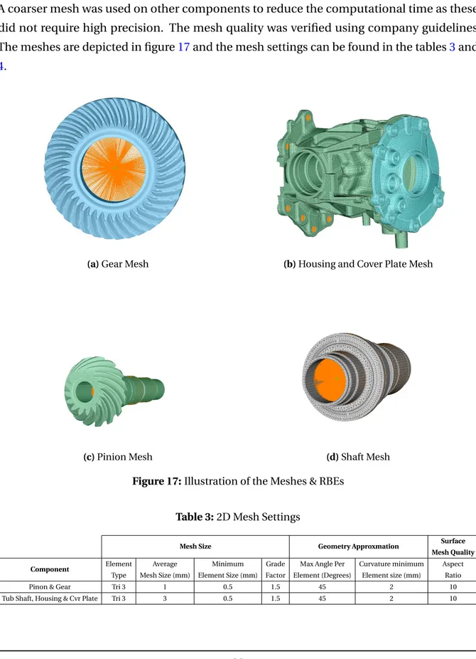
hand, an unnecessarily fine mesh will add a significant amount of time to the simulations. Since the TE must be accurately predicted, a finer mesh was used on the pinion and the gear. A coarser mesh was used on other components to reduce the computational time as these did not require high precision. The mesh quality was verified using company guidelines. The meshes are depicted in figure17and the mesh settings can be found in the tables3and

4.

(a) Gear Mesh (b) Housing and Cover Plate Mesh

(c) Pinion Mesh (d) Shaft Mesh

Figure 17: Illustration of the Meshes & RBEs

Table 3: 2D Mesh Settings

Mesh Size Geometry Approxmation Surface

Mesh Quality Component Element Type Average Mesh Size (mm) Minimum Element Size (mm) Grade Factor

Max Angle Per Element (Degrees)

Curvature minimum Element size (mm)

Aspect Ratio

Pinon & Gear Tri 3 1 0.5 1.5 45 2 10

(30)

Table 4: 3D Mesh Settings

Mesh Size Geometry Approxmation Quality

Component Element Type Average Mesh Size (mm) Internal Grading

Max Angle Per Element (Degrees) Curvature minimum Element size (mm) Tet Collapse Min Value Min Jacobian-Ratio Value

Pinon & Gear Tet 10 4 0.5 20 2 0.12 0.7

Tub Shaft, Housing & Cvr Plate Tet 10 4 0.5 20 2 0.12 0.7

After creating the mesh, the Rigid Body Element’s (RBE’s) were defined. RBE’s are geo-metrically rigid links which can be used to transfer load. There are two types of RBE’s, RBE2 and RBE3. The difference between them is that RBE2 distributes force and moments equally among all connected nodes. Figure18aillustrates this using a force of 100 N. On the other hand, RBE3 distributes the load based on the distance, this can be observed in figure

18b.

RBE’s are used in this thesis for several reasons. As previously mentioned, they can be used to transfer loads. Secondly, they can be used to represent a bolted connection if it is known that the bolt will not fail under the applied load. Thirdly, they can be used as connection points. The RBE’s will be identified as interface nodes in Adams, enabling them to be used as connection points. These interface nodes became points where the location and direction of joints, bearings, forces and torques were defined. The mesh for each component, as well as RBEs, can be seen in figure17. The final step was to export the files in the BDF format.

(a) RBE2 (b) RBE3

Figure 18: The Difference Between RBE2 and RBE3

3.2.2 Generating Flexible Bodies

In this thesis, the program MSC Marc was used to generate the Modal Neutral Files (MNF’s). MNF’s are a type of file format which contain the data of a flexible body. The files contain

(31)

information such as the inertia matrix, the mode shapes and their frequencies. These are obtained through an eigenfrequency analysis. However, a Craig-Bampton modal synthesis is required because it reduces the DOF, reducing computational time, yet still captures the elasticity of parts. The MNF’s were created using the following steps:

1. Imported the BDF files created in SimLab 2. Mass properties of each part were specified

3. Geometric properties of the CAD files were inserted (i.e. units) 4. (Glue contact created between the housing and cover plate) 5. The free-set DOF were selected, where RBE’s were defined 6. A Craig-Bampton analysis was created

7. MNF file was chosen as the desired output

An extra step was added when the external housing was considered because the Adams2Actran plugin only supports the analysis of one MNF. Therefore, a glue contact was generated be-tween the housing and cover plate using the contact tables feature. When generating the glue contact, it was ensured that the stress-free initial contact was selected. This method is viable under the assumption that the mass of the bolts is not significant and the assembly can be considered as sufficiently clamped. A further benefit is that this closely resembles the method used to fixate the PTU during testing. This can be seen in figure19. It can be observed that the housing side of the PTU is fixated to the test-rig, whereas the cover plate has been clamped using only the bolts.

(32)

Figure 19: PTU Mounted in the Test Rig [1]

3.3 Multi-body Dynamics

3.3.1 The Program

In Adams, a body refers to the individual geometry of each subcomponent that make up the PTU, i.e. pinion, shaft, housing, cover plate, etc. Idealised joints and forces are added to the bodies which affect how forces are translated throughout the system. Contact instances are made between areas that are in contact during the simulation to calculate the forces and motions between them. Finally, motions and external forces are added to the model to represent the load cases. Multibody dynamic simulations work by solving a system of Differential-Algebraic Equations (DAE) to calculate the position, acceleration and velocity on each body [26].

3.3.2 Flexible Bodies

Rigid body dynamics are commonly used when dealing with multi-body systems. However, introducing flexibility into the system can improve simulations by capturing the system’s frequencies more accurately, thus producing more reliable results. When considering NVH behaviours, flexible bodies are required because some elastic deformation must occur for vibrations to propagate through a system [27]. Consequently, flexible bodies can more

(33)

accurately predict the inertial properties and compliance. Therefore, all the sub-components of the PTU were required to be flexible bodies. Adams utilises flexible bodies through MNFs. The equation of motion for flexible bodies can be calculated from the Lagrange equation [28] (see equations8 and 9). Please consult [28] for further details on the mathematics involved. d d t µ∂L ∂ζ ¶ −∂L ∂ζ+ ∂E ∂ζ + µ∂Ψ ∂ζ ¶T λ −Q = 0 (8) Ψ = 0 (9)

where: L = Lagrange item = Kinetic Energy (T) - Potential Energy (V)

ζ = The generalised coordinates E = The energy dissipation function

Ψ = The constraint equations

λ = Lagrange multipliers for the constrains Q = Generalised applied forces

3.3.3 Modelling Process in Adams

In short, the following steps were taken to generate the results from the MBD model : 1. Imported the MNFs of the gear, tubular shaft and pinion

2. Added idealised joints

3. Added contacts between the pinion and the gear 4. Applied the motion and resistive torque

5. Added the bearings

6. Added the MNF of the housing and cover plate (one MNF) 7. Added bushings at bolt locations

8. Added markers and desired output calculations (e.g. TE) 9. Simulated the different load cases

(34)

Firstly, the unit system of Adams was set to match those from the meshing process (mm, kg, N, Deg, S). The files were individually imported using the create flexible body function. There were several options for the inertia modelling. Adam’s utilises nine inertia invariants to calculate the time-varying mass matrix of a flexible body. The invariants are calculated by analysing each nodes mass, undeformed location and participation in component modes [29]. The most applicable two were full-coupling and partial-coupling. The difference between them is that in full-coupling, more invariants are activated, which results in more precise results. However, this significantly increases computational time for all simulations. Therefore, after a short study, all components were loaded with the inertia set to partial-coupling as it provided a good balance between speed and precision.

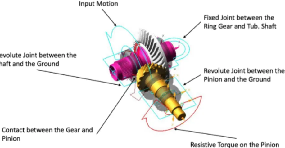
The boundary conditions were modelled using the joint, joint motions, bushings and torque functions. First, a fixed joint is used to attach the gear to the shaft. Secondly, a revolute joint is used to attach the shaft to the ground to enable it to rotate in the direction of the applied motion from the gearbox. The motion is applied at an interface node on the shaft. Next, the pinion is attached to the ground using a revolute joint which enables it to turn when it is excited by the gear. The joining methods can be observed in table5. A contact was created between the pinion and the gear. Finally, a resistive torque was placed on the pinion at an interface node.

It was crucial to define the contact between the gear and the pinion correctly. Therefore, it was important to conduct a study to calculate the best input parameters which yield reliable results but are not computationally expensive. This was particularly important when the bearings were added, as these greatly increased the computational time. The contact settings can be found in table6in section3.3.4. At this stage, a simple hypoid gear model was created, as seen in figure20.

(35)

Figure 20: Labelled Hypoid Gear Model

Table 5: Joining Methods

Parts Joining Method

Housing - Ground Bushings Tubular Shaft - Ground Revolute Joints Ring Gear - Tubular Shaft Fixed Joint

Pinion - Ground Revolute Joint Pinion - Ring Gear Contact

The bearings were created using the BearingAT module, which required highly detailed and specific dimensioning. The bearings were attached at the interference nodes (i.e. RBE locations). The locations of the bearings can be found in figure21. Bearing B11 and B12 were located on the pinion, whereas, bearings B22 left and right were located on the tubular shaft. Note, bearings B22 left and B22 right had the same dimensions.

(36)

Figure 21: Locations of the Different Bearings

Initially, the housing was imported and fixed joints were used at bolting locations, on the same side, as shown in figure19. However, it was later discovered that the fixed joints made the model unrealistically stiff, resulting in incorrect housing accelerations. The stiffness was due to the joints being idealised to an infinite stiffness. In reality, joints have more compliance which is important for a vibration response analysis. Hence, bushings were created at bolting locations with a very large stiffness of 1E 9. This method was beneficial as it enabled some compliance in the system, thus correlating better with experimental results.

Finally, markers were placed onto the housing, shaft and pinion. These were used to calculate different quantities using the create function measure utility in Adams. Key quantities that were measured were the pinion and shaft speed (in rpm) and the angular positions of the gear and pinion, to calculate the TE as defined by equation3. A marker was placed on the housing at the same location as an accelerometer used in testing. The accelerometer and bushing placements can be observed in figure22.

(37)

Figure 22: Accelerometer Placement and Bushing Placement

3.3.4 Contact Mechanics

The contact was created using the IMPACT function in Adams. A simple example of the IMPACT function can be seen in figure23. In this example, a ball is falling to the ground. If the distance between the I and J markers reaches x1, the IMPACT function comes into effect. However, if the distance between the I and J markers is greater than x1, the force is zero [30].

The IMPACT function consists of a spring component (k) and a damping component (c). The stiffness component is proportional to the stiffness coefficient (stiffness per unit length). Therefore, this changes as the distance between the I and J markers change. The damping component opposes the direction of motion and reaches the selected maximum value at the specified penetration depth [30]. The equation defining the IMPACT function can be observed in equation10.

(38)

Figure 23: An Example of the IMPACT Function. A Ball Falling to the Ground [30]

IMPACT =   

M ax(0, k(x1− s)2− ST EP (x, x1− d,Cmax, x1, 0). ˙x) forx ≤ x1

0 forx ≥ x1

(10)

Initially, the contact between the gear and pinion was modelled using Hertzian contact theory, similar to other studies in the area [4]. However, as the contact settings had a significant effect on the results obtained, thorough investigations were conducted to adapt them to correlate better with real-life test results. An important consideration was the time it took for simulations to complete, particularly after the addition of the bearings. Therefore, the settings were fine-tuned to find a balance between speed and accuracy. The settings for the contact can be found in table6. It must be noted that some further optimisation may be required for other tests. In some analyses, the settings were tuned even further to correlate better with test results.

Table 6: Contact Settings

Setting Value

Stiffness 2E+5 Force Exponent 2

Damping 52

(39)

3.3.5 Solver

Table7shows the solver settings used for all MBD simulations. These settings were selected as it had the best balance between speed and precision.

Table 7: Solver Settings

Setting

Value

Integrator

HHT

Formulation

I3

Hmax

1E-3

Interpolate

Yes

3.4 Acoustic Simulations

3.4.1 Acoustic Pre-Processing

The Adams2Actran plugin can use either the displacement/velocity/acceleration, or the modes and participation factors of the component as an input to calculate the acoustic behaviour. This feature is beneficial because the number of calculations required to be computed in Adams is reduced, which significantly reduces the computational time. A further benefit is that the results files are smaller, which reduces the latency within the Adams interface. A shrinkwrap mesh is required to do this in the frequency domain. For radiation analyses in air, one-way coupling is assumed.

The Adams2Actran plugin can create the acoustic meshes (see section2.4) automatically for simple geometries. However, the PTU was too complex, causing the automatic meshing to fail. Therefore, it was necessary to create the shrinkwrap mesh manually. This was done in the Actran interface.

The wavelength computation tool within Actran was used to determine the size of the mesh required. The maximum frequency to be analysed was a key parameter. To simulate up to 2000 Hz an element size of 28.3 mm was required. An essential requirement for the shrink wrap is that it cannot enter the original mesh through holes and crevices because the vibrations will not be captured correctly. Therefore, all holes needed to be filled.

To manually fill the remaining holes, the ’fill holes’ option was utilised in the Actran UI. How-ever, this did not successfully fill all the gaps in the housing. To manually fill the remaining

(40)

holes, the surface mesh option was used. After all holes were filled, the exterior shrinkwrap function was used to generate the shrinkwrap. It was crucial to ensure the shrinkwrap did not intersect itself and did not enter any holes.

The projection quality of the shrinkwrap was analysed to assess the quality of the shrinkwrap. A localisation percentage shows the ratio of structure nodes projected. The aim was to get as close to 100% as possible. The shrink wrap created had a localisation percentage of 92%. This was achieved using a mesh size of 10 mm as 28.3 mm was not adequately fine enough to capture the complex geometry of the PTU. The shrinkwrap can be observed in figure

24.

Figure 24: The Shrinkwrap

3.4.2 Creating the Analysis

First, a frequency domain analysis was created as time-domain analyses are more appropriate for transient cases and will result in large files due to the amount of information which would be stored. Next, the BDF and MNF files of the housing, the simulation name and time range to be analysed were specified. Note, the BDF and MNF files must be in the same folder with the same name. When creating the analysis a field is created asking for the steps to skip. This steps to skip is dependent on the Nyquist criterion and can be calculated as shown in equation11.

(41)

Steps to Skip = µ_t N y qui st tAd ams ¶ − 1 (11)

where: tN y qui st = 1/(2 ∗ Max frequency to be analysed)

tAd ams = Time step used in Adams

In this thesis, the max frequency that was analysed was 2000 Hz and the time step used in Adams was 2.5E − 4. Therefore, the steps to skip was zero.

3.4.3 Analysis Setup

The analysis setup settings can be observed in table8. Here, the gap tolerance was specified, whether an output map should be generated and the memory settings, note -1 means all available memory. In this analysis, an output map step was not created due to computa-tional limitations as this requires significant amounts of computacomputa-tional power, memory and time.

Table 8: Analysis Setup

Setting Gap Tolerance 0.01 m

Output Map No Output Map Steps N/A

Memory -1

3.4.4 Far Field Setup

Please consult section2.2.4for the definition of far field. The order of infinite elements is used to compute the SPL outside the finite element area. The infinite elements can be considered as a polynomial with several interpolation points, equal to the order of infinite elements. A higher-order will increase the accuracy of the infinite elements and the simulation. However, this will also significantly increase the computational time. An order of ten was used in this analysis as this setting produced the best results despite requiring more computational time. A graphical representation of the infinite elements can be seen in figure25. The microphones used for post-processing in terms of SPL can be specified here. As explained in section2.4, it is difficult to compare results in terms of SPL directly. Therefore, SWL was used. Microphone

(42)

Figure 25: Graphical Representation of the Infinite Elements (outside the blue circle) [31]

selection was based on ISO standards for radiation testing. The settings used can be seen in table9.

Table 9: Far-Field Setup

Setting Order of Infinite Elements 10

Microphone Table ISO (default) Translation of Microphone Centre 0,0,0

Scale Factor for Microphones 1 Microphones for Post-Processing 40

3.4.5 Environment Setup

Table10displays the environment settings used in this thesis. Table 10: Environment Settings

Setting Acoustic Environment Air at 15 °C

Speed of Sound 340 m/s Fluid Density 1.22 kg/m3

3.4.6 Analysis Parameters

The Discrete Fourier Transform (DFT) settings dictate the properties of the DFT which transform the vibrations of the flexible body from the time domain to the frequency domain.

(43)

The time interval determines the resolution of the analysis. The overlap percentage is required to obtain better-looking waterfall diagrams. A time interval of 0.1 is recommended for this analysis. If the time interval is too high, the results do not conform correctly. On the other hand, if the interval is too low, then any noise will greatly impact the results. Some trial and error may be required to determine the best parameters to use. The DFT settings can be found in table11. The parameter settings used in this study can be found in table 12. Time windowing defines the form of the window. The Hanning option, which is used in this analysis, is defined in equation12.

w (n) = 0.5 − 0.5cos µ 2πn M − 1 ¶ (12)

where: n = Number of sampling points

M = Quantity of same point in the window w = The window function

The frequency range that was to be analysed was selected. This must conform to the mesh size of the shrinkwrap and must be cross-referenced with the Nyquist criterion as explained in section3.4.2. The radiation frequencies for the green analysis defines the number of frequencies used for the step in the green analysis (radiation analysis). The higher the number, the better the accuracy. For this analysis, four radiation frequencies was used. The number of bands for adaptive volume mesh defines the number of frequency ranges used for the adaptive mesh. The relative thickness for the perfectly matched layer corresponds to the number of acoustic wavelengths at the lower limit of each frequency band. The Hexa mesh option is selected because it creates a better mesh. In the event that the simulation fails at the meshing stage, this can be turned off. All of the analysis parameters are presented in table12.

Table 11: DFT Settings

Setting Time Windowing Hanning

Time Interval 0.1 s Overlap of Time Interval 50%

(44)

Table 12: Analysis Parameters

Setting Frequency Start 1 Hz Frequency Step 100 Hz Frequency End 2000 Hz Num of Radiation Frequencies for Green Analysis 4

Num of Bands for Adaptive Volume Mesh 6 Relative Thickness for the Perfectly Matched Layer 1 Use Hexa Mesh Yes

3.4.7 Mesh

The final step was to link the manually created shrinkwrap to the analysis, note all files must be in the same folder. Figure26illustrates the ISO configuration of microphones and the shrinkwrap within the Adams interface. Microphone 40 is highlighted in red.

Figure 26: The Shrinkwrap Within the Adams Interface

(MNF Conversion)

In the event that an MNF version error occurs during Adams2Actran simulations, the Flex toolkit provided by MSC can be used to covert the MNFs to a readable version by selecting the settings observed in figure27. This may occasionally occur due to the software and/or program version used to generate the MNFs being incompatible with Actran’s drivers.

(45)

(46)

4 Results and Analysis

This section presents the results obtained from the simulations and analyses them. Suggestions for future work are also presented.

4.1 Model Validation

To validate the model, several simulations were conducted within Adams and these were compared to test results previously conducted on the PTU in the testbeds. For example, the TE was tested at different speeds and torques. Furthermore, the housing acceleration response was measured at specific locations within Adams and compared to test data gathered through the use of accelerometers.

4.1.1 Transmission Error Validation

There were two different TE tests used to validate the model. The first test was an End-Of-Line (EOL) test, where a fully assembled unit was taken from the end of the assembly line and placed into the rig. The test was conducted at a speed of 60 rpm, from table1it can be inferred that the peak amplitude will occur at 15 Hz. The amplitude of the signal at the first fundamental frequency and first harmonic were measured inµRad. An FFT of the TE signal was performed within Adams to obtain comparable results. Figure28shows the simulated results obtained from Adams. Table13compares the simulated results with the EOL test.

(47)

Figure 28: End of Life Simulated Results

Table 13: Comparison of the TE Between the EOL Test and Simulated Results

Frequency (Hz) Simulated Results (uRad) Test Results (uRad)

15 27 28

30 6 5

Further TE tests were compared to the simulated results to ensure that the model was valid when varying the torque. The tests were conducted at 15 Nm, 100 Nm and -15 Nm. Figures

29,30and31show the TE signal for the various torques. Table14shows a comparison of the first order TE values calculated from the simulation and the test results.

(48)

Figure 29: TE at 15 Nm

(49)

Figure 31: TE at -15 Nm

Table 14: Comparison of the First Order TE at Different Torques

TE First Order (uRad)

Torque (Nm) Minimum Value (Test) Maximum Value (Test) Simulated Result

15 4.5 20 16.9

100 7.9 15.8 13.5

-15 26 34 26.1

From table14, it can be observed that the model was able to predict the amplitude of the TE with an acceptable degree of accuracy as it is similar to the results observed in previous research [1]. The TE decreases as the torque increases, this occurs due to the overall stiffness of the model increases as the torque increases, resulting in better gear meshing and thus less TE fluctuations.

4.1.2 Housing Vibration Validation

To test the vibration of the housing, an accelerometer was placed onto the housing at a specific location, as specified in figure32. A speed ramp cycle up to 2000 rpm is run, i.e. the test starts at 0 rpm and gradually increases to 2000 rpm where it stays constant for some time

(50)

and returns slowly back to 0 rpm. In Adams, this was achieved by placing a marker at the same location and creating measures to capture the acceleration at that point.

Figure 32: Accelerometer Location

The vibration was analysed in terms of the Power Spectral Density (PSD). PSD is defined as the squared value of a signal. It describes the power of a signal or time series distributed over different frequencies. A PSD is an FFT which converts a time-domain signal to a frequency-domain signal [32]. The shape of the PSD plot defines the average acceleration of the signal at any frequency. Figure33displays the test results. On the other hand, figures34-37show the simulated results obtained in Adams.

(51)

Figure 33: Housing Accelerations at 2000 rpm from Testing

From the test data (figure33), the largest peak was observed at 1000 Hz in the Y direction, and the Y direction remains dominant at 1400 Hz. The largest amplitude at 500 Hz is in the Z direction and lowest in Y. The amplitude of the accelerations in the Z direction decrease as frequency increases and becomes very low in comparison to the other directions. There is only a small peak in all directions at 2000 Hz and this tends towards zero as the frequency reaches 2500 Hz.

(52)

Figure 34: Simulated Housing Acceleration in the X Direction at 2000 rpm

Figure34displays the simulated results of the housing acceleration in the X-direction. It can be observed that the simulation correctly predicted the fundamental frequencies which excited the component, i.e. 500, 1000 and 1500 Hz (as predicted in table1). However, the shape of the peaks does not directly match the experimental results. This discrepancy may be due to the difference in damping between the model and reality or a difference in the frequency resolution. Investigations should be conducted to decouple the contact parameters in terms of housing vibrations.

Figure35highlights that the simulation can predict the shape of the PSD curves correctly. The largest peak in all directions occurs at 1000 Hz. However, in the test data, the Y component retains the largest amplitudes at 1500 Hz. In the simulated data, this is in the X direction instead.

From figure36, it can be observed that the simulation correctly predicted that the acceleration in the Z direction would be relatively low in comparison to the X and Y directions above 500 Hz. The simulation was unable able to predict that the largest amplitude, in the Z direction, was at 500 Hz. However, the amplitudes do decrease at 1500 Hz. Overall, the simulation was able to predict what happens to an acceptable degree of accuracy.

(53)

Figure 35: Simulated Housing Acceleration in the Y Direction at 2000 rpm

(54)

Figure 37: Comparison of the Simulated Housing Acceleration in All Directions at 2000 rpm

From figure37, it can be observed that the simulated system is sensitive to large accelerations at 500, 1000 and 1500 Hz, whereas the test data shows large displacements at 510, 1028 and 1410 Hz. Overall, the simulation predicted the general shape of the accelerations to an acceptable level. However, the amplitude of the simulated and test results do not match exactly. A key contributor to the discrepancy, in addition to those already mentioned, is that the simulations were conducted during a very short time span due to computational limitations and time constraints. In contrast, the test data was gathered over approximately 30 seconds, enabling the speed to increase smoothly, steadily and controllably. A smoother ramp-up would naturally cause lower amplitudes. This is comparable to speeding up from 0-60 mph (0-100 km/h) within two seconds or speeding up within 10 seconds in a passenger vehicle. The faster the car accelerates, the more the car vibrates and vice-versa.

In the future, extensive research should be conducted to decouple contact parameters and damping ratios to understand each of their effects on the housing accelerations. Once this has been validated, and assuming the required computational power is available, a simulation should be conducted which directly follows the testing protocol, i.e. ramps-up slower and is simulated for 30 seconds.

(55)

directions, for each frequency, was summed up and plotted in a bar graph. This was achieved by using the vector sum formula, as presented in equation13. The results for the experimental data can be found in figure38and the bar graph for the simulated results can be seen in figure39.

Vector Sum = q

x2_{+ y}2_{+ z}2 ₍₁₃₎

(56)

Figure 39: Vector Sum of the Simulated Housing Accelerations

From comparing the vector sum of the experimental and simulated results (figures38and39), it is evident that the simulation correctly predicted the overall trend of the housing vibrations. A lower amplitude is observed at 500 Hz. Meanwhile, the highest is at 1000 Hz and 1500 Hz sits somewhere in-between. It is observed that overall, the simulation was very accurate in predicting the total vibration. Using this information, it can be inferred that the acoustic simulations will show the largest excitations at 1000 Hz and the least at 500 Hz.

4.2 Acoustic Simulations

Figure40presents the waterfall diagram of the SWL. The system excitations are clearly visible at 500, 1000 and 1500 Hz. This corroborates with the findings from the experimental data and simulated data which evidenced large housing vibrations at these frequencies. As predicted from the vector sum graphs, the most noise occurs at 1000 Hz because this is the frequency that is most excited at 2000 rpm, the SWL is approximately 50 dB. At 500 Hz, the sound power is lower, due to less housing vibrations occurring at this frequency. The sound power at 1500 Hz lies between the other two, which is in line with the results from figures38and39.

(57)

Figure 40: Waterfall Diagram Displaying the Simulated Sound Power Level (SWL) at 2000 rpm

The Overall Sound Power Level (OSWL) value throughout the simulation can be observed in figure41. This shows that as the simulation speeds up to 2000 rpm, the OSWL increases and the curve flattens at approximately 64 dB. The OSWL is calculated in Actran using equation

14. The OSWL is higher than the values shown in the waterfall diagram because it considers the entire spectrum.

Figure 41: Output Sound Power Level

OSW Ld B= 10l og r Rfmax fmi n W 2_{d f} Wr e f (14)