Investigation of driver sleepiness in FOT data : final report of the project SleepEYE II, part 2

(1)

Investigation of driver sleepiness

in FOT data

Final report of the project SleepEYE II, part 2

ViP publication 2013-2

Authors

Carina Fors, VTI David Hallvig, VTI

Emanuel Hasselberg, Smart Eye Jordanka Kovaceva, Volvo Cars

Per Sörner, Smart Eye Martin Krantz, Smart Eye John-Fredrik Grönvall, Volvo Cars

(2)

(3)

Preface

SleepEYE was a collaborative project between Smart Eye, Volvo Cars and VTI (the Swedish National Road and Transport Research Institute) within the competence centre Virtual Prototyping and Assessment by Simulation (ViP). The project was carried out during the years 2009–2011, and included development of a camera-based system for driver impairment detection and development of a driver sleepiness classifier adapted for driving simulators.

A continuation project called SleepEYE II was initiated in 2011. This project has included three work packages: 1) simulator validation with respect to driver sleepiness, 2) assessment of driver sleepiness in the euroFOT database using the camera system that was developed in SleepEYE, and 3) further development and refinement of the camera system. The present report documents the work that has been undertaken in work packages 2 and 3 of SleepEYE II.

John-Fredrik Grönvall at Volvo Cars has been the project manager, and Jordanka Kovaceva, also Volvo Cars, has been responsible for all tasks related to the euroFOT database.

Martin Krantz, Emanuel Hasselberg and Per Sörner at Smart Eye have done all work in work package 3 and also contributed to the data processing in work package 2.

Anna Anund, Carina Fors and David Hallvig at VTI have been responsible for developing and evaluating the methodologies used in work package 2. Beatrice Söderström, VTI, recruited participants to the video experiment.

Katja Kircher at VTI, Julia Werneke and Jonas Bärgman at SAFER (the Vehicle and Traffic Safety Centre at Chalmers) have reviewed the report and given valuable feedback on the content.

The SleepEYE II project was financed by the competence centres ViP and SAFER (Vehicle and Traffic Safety Centre at Chalmers).

Thanks to all of you who have contributed to the project.

Linköping, December 2012

(4)

Quality review

Peer review was performed on 26 October 2012 by Julia Werneke and Jonas Bärgman, SAFER (the Vehicle and Traffic Safety Centre at Chalmers) and on 9 November 2012 by Katja Kircher, VTI. Carina Fors has made alterations to the final manuscript of the report. The ViP Director Lena Nilsson examined and approved the report for

(5)

Investigation of driver sleepiness in FOT data

by Carina Fors1_{, David Hallvig}1_{, Emanuel Hasselberg}2_{, Jordanka Kovaceva}3_{, Per} Sörner2, Martin Krantz2, John-Fredrik Grönvall3, Anna Anund1

1_{VTI (Swedish National Road and Transport Research Institute)} 2_{Smart Eye}

3_{Volvo Cars}

Executive summary

Driver sleepiness contributes to a great number of motor vehicle accidents every year. In order to reduce the number of sleepiness related accidents, more knowledge on e.g. prevalence, countermeasures and driver behaviour is needed. Data from field

operational tests (FOT) has a potential to provide such knowledge with high ecological validity.

The objective of the project was to propose and evaluate methods for identification of driver sleepiness in FOT data. More specifically, the aim was to identify objective indicators of sleepiness – based on driving behaviour, eye blink behaviour and models of circadian rhythm – and to evaluate a subjective video scoring method for estimating driver sleepiness levels. Data from two separate projects were used: 1) the ViP-project SleepEYE, in which a controlled field test was conducted, and 2) euroFOT, which was a large scale FOT.

In a first step the data quality of blink-based indicators obtained from a camera system was evaluated. It was concluded that the data quality had to be improved and thus, a new detection algorithm was devised and implemented. The new detection algorithm had an acceptable detection rate (approximately 50 %) when applied to data from the SleepEYE field test, but for euroFOT data the number of identified blinks was very low (< 5 blinks/min) in about half of the trips. There is thus a need for further improvements of the blink detection algorithm.

An in-depth study on indicators of driver sleepiness was carried out using data collected in the SleepEYE experiment, with the purpose of employing the best indicators to study driver sleepiness in the euroFOT database. The most promising indicators were found to be mean blink duration and number of line crossings. A sleepiness classifier was

suggested based on the distribution of the data (i.e. visual inspection). When applied to SleepEYE data the classifier was found to have good specificity while the sensitivity of the classifier was not so good. From euroFOT no true data on the drivers’ sleepiness levels were available and it was therefore not possible to evaluate the performance of the classifier. However, an explorative analysis showed that only very few data points were classified as sleepy. This may be reasonable since most trips were conducted during daytime, but it is a somewhat disappointing result for the project.

A study was carried out on whether it is possible to use video recordings of drivers in order to estimate the drivers’ self-rated level of sleepiness. Forty participants rated 54 one-minute video clips of an equal number of sleepy and alert drivers on a scale with three levels (alert, first signs of sleepiness, very sleepy). The results of the study showed that performing such observer rated sleepiness (ORS) estimations on drivers is

(8)

which, clearly limits the possibility of making reliable observer rated sleepiness estimations.

In conclusion, studying driver sleepiness in (existing) FOT data is difficult, for several reasons: 1) eye camera based indicators suffer from detection errors and low detection rate, 2) driving-based indicators are influenced by e.g. road curvature and traffic

density, 3) models of sleepiness cannot be used since no information on hours slept and time awake is available, and 4) video scoring is not reliable, at least not given the quality of the available video recordings.

In future studies on driver sleepiness in FOTs sleepiness should be addressed in the FOT design. Some information about the drivers' sleep and sleepiness (ratings, sleep diaries, etc.) must be collected during the test; otherwise it will be very difficult to get any useful results.

(9)

1 Introduction

Driver sleepiness contributes to a great number of motor vehicle accidents (NTSB 1999; Akerstedt 2000). In the UK the proportion of sleep related vehicle accidents has been estimated to about 10-20%, where the higher percentage refers to motorway (Horne & Reyner 1995; Maycock 1997). A study carried out in France found that, approximately, 10% of single vehicle accidents are related to sleepiness (Philip, Vervialle et al. 2001) whereas studies in Finland estimate that sleepiness is a contributing factor in 15% of fatal accidents caused by nonprofessional drivers (Radun & Summala 2004). A recent in-depth study of databases of crashes in the US between 1999 and 2008 concluded that an estimated 7% of all crashes and 16.5% of fatal crashes involved a sleepy driver (Tefft 2012). Compared to other police reported crashes, sleep related crashes are associated with a higher risk of death and severe injury (Horne & Reyner 1995).

A fundamental problem when studying driver sleepiness is, in fact, how to measure sleepiness. In short, the essence of the problem is that although an intuitive

understanding of sleepiness is rather self-evident to most people, the scientific concept is not so easily defined and it is not possible to directly measure sleepiness (Cluydts, De Valck et al. 2002). Sleepiness is therefore regarded as a hypothetical construction, which leads to the problem of operationalization (Maccorquodale & Meehl 1948). Different approaches to measuring sleepiness have been proposed and considered in the literature on driver sleepiness. According to Liu et al. (2009), some of the most

commonly studied approaches are: (1) subjective sleepiness estimates, (2) physiological measures, and (3) driving behaviour based measures.

Most research on driving while sleepy has been done in driving simulators (Liu, Hosking et al. 2009). In such driving simulator studies it has, for example, been found that subjective self-rated sleepiness is higher after sleep loss and during night-time driving (Gillberg, Kecklund et al. 1996; Åkerstedt, Peters et al. 2005) as well as that driver sleepiness is associated with (and likely causes) increased lateral variability (Anund, Kecklund et al. 2008; Lowden, Anund et al. 2009) which also results in an increased number of line crossings (Reyner & Horne 1998; Ingre, Åkerstedt et al. 2006). The absence of any real risk in the driving simulators is of course one of the major reasons why sleepiness is studied in simulators. However, the absence of any real risk may also be a drawback since it may have an influence on driving behaviour, and therefore make generalization, of results found in simulator studies to real world driving, invalid. This has motivated the studying of validity of driving simulators with regard to driver sleepiness. Although the results from various validation studies are somewhat different, sleepiness and the effects of sleepiness tend to be more pronounced in the simulator than on the real road, except for extremely long driving sessions, which might be explained by ceiling effects (Philip, Sagaspe et al. 2005b; Sandberg, Anund et al. 2011b; Davenne, Lericollais et al. 2012).

Driving performance and sleepiness have also been studied in controlled experiments on real roads, where sleep deprivation has been found to be associated with increased subjective sleepiness (Philip, Sagaspe et al. 2005a; Sandberg, Anund et al. 2011a) and an increased number of line crossings (Philip, Sagaspe et al. 2005a; Sagaspe, Taillard et al. 2008). Driver sleepiness has also been shown to have a relationship with

electroencephalographic (EEG) activity (Kecklund & Åkerstedt 1993; Sandberg, Anund et al. 2011a; Simon, Schmidt et al. 2011), blink duration (Häkkänen, Summala et al. 1999; Sandberg, Anund et al. 2011a) and speed (Sandberg, Anund et al. 2011a). An

(10)

overview of indicators and methods for detection of driver sleepiness can be found in a previous SleepEYE report (Fors, Ahlström et al. 2011).

A limitation of the research methodologies mentioned above is that they either rely on drivers’ self-reported experiences of sleepy driving or reflect driving behaviour in an artificial setting where the driver is being monitored. To what extent the results from such studies can be generalized to real world driving is not fully known. Therefore, other research methods are needed in order to validate and to supplement these results. In recent years, several large scale naturalistic driving studies (NDS) and field

operational tests (FOT) have been conducted to better understand drivers' behaviour. In these studies drivers are unobtrusively monitored in a natural driving setting, often for a relatively long time. The objectives of NDS/FOT studies are often to study the effects of driver assistance systems or to analyse accidents and incidents. However, NDS/FOT studies are also of interest from a sleepiness perspective, for several reasons. First, driver behaviour can be investigated without any influence from a test leader or a test protocol. Second, risk factors and prevalence of driver sleepiness could potentially be studied. It might also be possible to identify countermeasures used by sleepy drivers and to evaluate the effect of those.

Since NDS/FOT studies are not controlled experiments, conventional analysis methods cannot be used. A key issue is the lack of reference values (e.g. self-reported subjective sleepiness) or well-defined conditions (e.g. alert vs. sleep deprived). Thus, in order to use NDS/FOT data for sleepiness research, new and/or modified analysis methods are needed.

There have been a few attempts to investigate driver sleepiness using NDS/FOT data reported in the literature. Barr and colleagues have identified and characterized driver sleepiness among truck drivers in a naturalistic driving study (Barr, Yang et al. 2005). The entire video library was reviewed by a video analyst who rated the drivers’ sleepiness levels on a five-point scale. A subset of the sleepiness events was then analysed in detail. A different methodology was used by Dingus and colleagues (Dingus, Neale et al. 2006). Instead of reviewing all video data a number of triggers were defined and implemented in the data acquisition system. Whenever a trigger criterion was fulfilled, the acquisition system recorded video and driving data for a short time period of 90 s before and 30 s after the triggering event. The collected videos were then reviewed by video analysts who categorized the events and rated the drivers’ sleepiness levels. The rating scale used in both studies was based on the Observer Rating of Drowsiness (ORD) proposed by Wierwille and Ellsworth (Wierwille & Ellsworth 1994). The ORD scale is a 5-grade scale ranging from "Not drowsy" to "Extremely drowsy". There are two major limitations with the ORD scale (see also Chapter 5): 1) there is no guidance on how to use and interpret the scale, i.e. the ratings will depend on the rater's own interpretation, and 2) the scale has not been validated to any "true drowsiness level". There is thus a need for a validated video scoring method. The objective of the present project, SleepEYE II, was to propose and evaluate methods for the analysis of driver sleepiness in FOT data. More specifically, the aim was to identify objective indicators of sleepiness and evaluate a subjective video scoring method for estimating driver sleepiness levels. Data from two separate projects were used: 1) SleepEYE, in which a controlled field test was conducted, and 2) euroFOT, which was a large scale field operational test conducted in the years 2008–2011. The SleepEYE II project included three work packages. Work package 1 aimed at conducting a simulator validation study using data from the SleepEYE experiments.

(11)

The results from that study are presented in a separate report (Fors, Ahlström et al. 2013). Work package 2 concerned the methodologies for analysing driver sleepiness in FOT data, as described above. In work package 3, the embedded 1-camera system that was developed in SleepEYE was further improved. The present report constitutes the documentation of work packages 2 and 3.

1.1 The SleepEYE I project

The present project is a continuation of the SleepEYE project (which will be referred to as SleepEYE I from now on). The aims of SleepEYE I were to develop and evaluate a low cost eye tracker unit, to identify sleepiness indicators feasible for use in driving simulators, to determine indicator thresholds for sleepiness detection, and to combine the indicators into a simple classifier (Fors, Ahlström et al. 2011).

SleepEYE I began with a literature review on indicators for driver sleepiness and distraction. The following parts of the project were then focused on driver sleepiness. The most promising indicators for use in driving simulators were found to be blink duration, percentage of eyelid closure (PERCLOS), blink frequency, lateral position variation, and predicted sleepiness level based on a mathematical model of wakefulness and sleep. The eye related indicators were implemented in a 1-camera embedded eye tracker unit that was especially designed to be used in vehicles.

The project included two experiments. The first was a field test where 18 participants took part in one alert and one sleepy driving session (as defined by time of day) on a motorway. 16 of the 18 participants also participated in the second experiment which was a simulator study similar to the field test. Data from the eye tracker, from

physiological sensors, and from the vehicle were continuously registered during the driving sessions.

The field test data were used for evaluation of the 1-camera system with respect to the sleepiness indicators. Blink parameters from the 1-camera system were compared to blink parameters obtained from a reference 3-camera system and from the electrooculo-gram (EOG). It was found that the 1-camera system missed many blinks and that the blink duration was not in agreement with the blink duration obtained from the EOG and from the reference 3-camera system. However, the results also indicated that it should be possible to improve the blink detection algorithm since the raw data looked well in many cases where the algorithm failed to identify blinks.

The sleepiness classifier was created using data from the simulator experiment. In a first step, variants of the indicators identified in the literature review were implemented and evaluated. The most promising indicators were then used as inputs to the classifier. The final set of indicators was thus used to estimate a sleepiness level. The indicators were based on the Karolinska sleepiness score (KSS) value the driver reported before the driving session (KSSestSR), standard deviation of lateral position (SDLP), and fraction of blinks > 0.15 s (fracBlinks, for EOG-based and 1-camera based). An optimal

threshold for discriminating between KSS above and below 7.5 was determined for each indicator. The performances were in the range of 0.68-0.76.

Two decision trees based on the selected indicators were created: one using

fracBlinksEOG and one using fracBlinks1CAM. The performances of the two trees were 0.82 and 0.86, respectively (on the training dataset), i.e. the overall performance of the EOG based and the 1-camera based classifier were similar, although individual

(12)

dataset from another study, which illustrates the difficulties in creating a generalized sleepiness classifier.

A detailed description of SleepEYE I can be found in the project report (Fors, Ahlström et al. 2011).

1.2 The euroFOT database

The euroFOT project was the first large scale European field operational test on active safety systems. The project included 28 partners and test fleets in four different

countries. Data have been collected from hundreds of vehicles during one year. The Swedish test fleet consisted of 100 passenger cars and 50 trucks, and it was operated by Volvo Cars, Volvo Technology and Chalmers. In the present project data from the Swedish passenger cars are used.

Data were collected during the private and occupational everyday driving by ordinary drivers. The data come from several sources, such as the in-vehicle data network (CAN), GPS, eye tracking, and video of the driver and vehicle surroundings (the

context). The software of the eye tracking system was upgraded during the course of the test. Blink detection was added in the end of the project, why only data from the last upgrade – version 21 – are relevant for the present project. From a total of 66750 trips in the (Swedish passenger car) euroFOT database 2442 trips satisfied the software version condition. The data come from 36 different drivers and correspond to 6836 minutes of driving.

Since euroFOT was a naturalistic study no data on the drivers’ sleepiness levels are available. The reason is mostly due to a wish to make the driving as natural as possible and to avoid interaction with the drivers. Using electrodes to measure sleepiness, or asking questions, or other types of obtrusive measures are therefore out of the question.

1.3 Aim

The aims of SleepEYE II, work packages 2 and 3, were to:

 Improve head rotation tracking and initialization logic for the camera system.

 Propose and evaluate sleepiness indicators suited for FOT data.

 Develop and evaluate a methodology for video scoring of driver sleepiness.

1.4 Report structure

The report begins with a chapter about the work that was done to improve the software of the camera system (Chapter 2). In Chapter 3.1, the blink data obtained from the new improved camera software is evaluated. It is concluded that the blink detection needs to be improved, which is done in Chapter 3.2. The blink data quality from the new

algorithm is evaluated in Chapter 3.3. Blink parameters and some other sleepiness indicators are evaluated in Chapter 4. In Chapter 5 the video scoring method is

described and evaluated. In Chapter 6 the developed and suggested methods are applied to euroFOT data (however, the video scoring method turned out to give very poor results and it was thus never used on euroFOT data). The methods are discussed, and some conclusions and recommendations for future studies are given in Chapter 7 shows

(13)

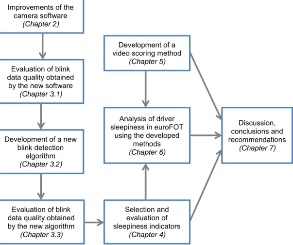
a flow chart of the work that has been undertaken within the project, and how the work has been structured in the report.

Figure 1: The flow chart shows the work that has been undertaken within the project, and how the work has been structured in the report.

1.5 Related publications

SleepEYE I resulted in three publications:

 Fors C, Ahlström C, Sörner P, Kovaceva J, Hasselberg E, Krantz M, Grönvall J-F, Kircher K, Anund A (2011). Camera-based sleepiness detection – Final report of the project Sleep EYE. ViP publication 2011-6, The Swedish National Road and Transport Research Institute, Linköping, Sweden.

 Ahlstrom C, Kircher K (2010). Review of real-time visual driver distraction detection algorithms. 7th International Conference on Measuring Behaviour, Eindhoven, Netherlands, 2010.

 Ahlstrom C, Kircher K, Sörner P (2011). A field test of eye tracking systems with one and three cameras. 2nd International Conference on Driver Distraction and Inattention, Gothenburg, Sweden, 2011.

Improvements of the camera software

(Chapter 2)

Evaluation of blink data quality obtained

by the new software (Chapter 3.1) Development of a new blink detection algorithm (Chapter 3.2) Evaluation of blink data quality obtained by the new algorithm

(Chapter 3.3) Selection and evaluation of sleepiness indicators (Chapter 4) Development of a video scoring method

(Chapter 5)

Analysis of driver sleepiness in euroFOT

using the developed methods (Chapter 6) Discussion, conclusions and recommendations (Chapter 7)

(14)

The first publication is the project report describing the experiments, the results of the camera evaluation with regard to blink parameters, and the sleepiness detector for driving simulators. The two following publications were produced outside the project, but are based on data from the project. In the first of these two publications the 1-camera system is compared with the 3-1-camera system with respect to gaze parameters. The second publication is based on the literature review on distraction indicators that was done within the project.

In SleepEYE II the work done in Work Package 1 has been published in a separate report:

 Fors C, Ahlström C, Anund A (2013). Simulator validation with respect to driver sleepiness and subjective experiences – Final report of the project SleepEYE II, part 1. ViP publication 2013-1, The Swedish National Road and Transport Research Institute, Linköping, Sweden.

In addition, the results of SleepEYE II were presented at a workshop in Gothenburg in June 2012. About 15 people from SAFER, Smart Eye, Volvo Cars and VTI participated in the workshop.

(15)

2 Improvements of the embedded camera system

Eyelid estimation is not possible without head tracking, and even if there is head tracking good estimation of the position and rotation of the head is needed for high quality eyelid measurements.

The existing software in the camera system has problems estimating the depth of the head position (i.e. the distance from the camera to the head). This is due to the fact that it is a 1-camera system. The problem makes it hard to track the rotation of the head because the position predicted by the system doesn’t correlate with the real position. Therefore it is hard to track horizontal head rotations larger than 10–15 degrees. A solution would be to adapt the system during tracking, i.e. when there is more information. This could unfortunately not be done on the embedded system due to the limited computational power.

Instead a solution where more tracking points were added was chosen, which gives a more robust estimation of the head rotation even if the estimated depth position of the head is not perfect.

2.1 Extended head rotation range

In order to extend the head rotation range beyond frontal and near frontal head poses, more feature tracking points need to be added. Good feature tracking points are corner-like, i.e. they can be identified both vertically and horizontally in the camera image. To find better tracking features for eyebrows and ears a new corner detector was

implemented. Due to the large computational requirements of the detector, the majority of time went into optimization. The resulting detector was able to find good corner points in a local region.

A significant effort also went into improvements of the head pose estimation algorithm, especially regarding its sensitivity to outliers, for example partial occlusions and mouth movements.

Improvements in other areas related to tracking have also been done.

Taken together, these and other improvements increased the horizontal head rotation range by approximately 10–20 degrees, depending on subject.

2.2 Improved initialization logic

The initialization mode of the eye tracker was improved and resulted in a much shorter time to tracking, which in turn improved the ability to initialize and track on highly mobile subjects. Most of the work was done to the state machine and lowered the requirements for a stationary head, without losing any tracking quality.

2.3 Improved tracking recovery

Tracking recovery is the state the eye tracker goes into when head tracking is lost, usually because of major occlusions or large head rotations. Tracking recovery is fast since a model of the head already exists, and is therefore preferred over initialization. For different reasons, the tracking recovery cannot always recover and a new

(16)

was previously constant. Improvements have now been made so that the time adapts to the length of time the eye tracker previously had good tracking of the face, balancing quick trashing of failed initializations against the survival of good tracking models. Improvements were also made to the tracking recovery algorithms, resulting in a quicker recovery.

(17)

3 Evaluation of blink data quality

The software of the embedded 1-camera system that was developed and evaluated with regard to blink parameters in SleepEYE I was further improved in the present project (see Chapter 2). The improved version was installed in the euroFOT cars during the last 1–2 months of the experiment. In order to have the best data possible, only data from that period were included in the present project.

As a first step, the performance of the new improved software version was evaluated with regard to its ability to detect blinks and to determine blink duration.

3.1 Evaluation of blink data from the camera system

3.1.1 SleepEYE field data

The 1-camera data that were acquired during the field test in SleepEYE I were re-run with the new version of the camera software and compared to blink data from the EOG. Relevant blink parameters were obtained from the EOG by the LAAS1_algorithm (Jammes, Sharabaty et al. 2008). In SleepEYE I the results showed that the LAAS algorithm had a detection rate of about 98%, which was considered to be good enough as a "ground truth" for evaluation of the camera blink detection algorithm.

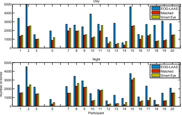
Figure 2 shows the number of blinks detected by LAAS and by the improved camera system per participant and driving session. On average, the camera system detects 39% of the number of blinks detected by LAAS (day: 41%, night: 36%). In two cases the camera system detects more blinks than LAAS. By comparing the camera detected blinks with the EOG, it is obvious that the camera data contains a lot of erroneous detections in these particular cases.

1_{LAAS is an abbreviation for Laboratoire d’Analyse et d’Architecture des Systèmes (Toulouse, France),}

(18)

Figure 2: Number of blinks detected by LAAS and by the camera system, respectively, subdivided into day and night-time. Participants 4 and 6 cancelled their participation and are thus not included in the analysis. Data from the SleepEYE I field experiment.

In order to obtain a more accurate comparison the individual blinks identified by the two systems were compared. First, the time delay between the blink signals was determined (from the cross correlation function) and adjusted for. For each blink identified by the camera system, a matching blink in the EOG was searched for in a time window starting 0.3 s before and ending 0.3 s after the start of the (camera) blink. When considering only matching blinks the camera system detects on average 32% of the blinks detected by LAAS (day: 32%, night: 33%). In about 2/3 of the driving sessions more than 90% of the blinks detected by the camera system could be matched to the LAAS detected blinks, which indicates that the number of erroneously detected blinks is fairly low in these sessions. However, in four driving sessions less than 60% of the blinks could be matched to the LAAS detected blinks. In one of these cases the detection rate was very low which implies that the camera system had problems detecting the blinks on the whole.

In the other three cases there were a lot of long blinks detected by the camera system. The fact that the blinks were long may explain the low rate of matching blinks (i.e. long blinks may not fit in the 0.6 s long search window). However, the reason why the blinks were long is that downward gazes were incorrectly identified as long eye closures. In another five driving sessions there were a lot of long blinks identified by the camera system that were matched to shorter blinks detected by LAAS. Also in these cases the long blinks could be explained by the fact that the camera system incorrectly had identified downward gazes as blinks (downward gazes are usually followed by a blink which explains why a shorter matching blink was found by LAAS). An example is shown in Figure 3. Another factor found to contribute to incorrect identification of long blinks is sunlight. Drivers that were exposed to sunlight tended to squint, which

probably made it difficult for the camera system to decide when the blink started and ended. 1 2 3 5 7 8 9 10 11 12 13 14 15 16 17 18 19 20 0 1000 2000 3000 4000 5000 Day 1 2 3 5 7 8 9 10 11 12 13 14 15 16 17 18 19 20 0 1000 2000 3000 4000 5000 Participant N u m b e r o f b li n ks Night EOG-LAAS Smart Eye

(19)

Figure 3: Example of a downward gaze that is incorrectly identified as a long blink. Note that there is approximately 1 s time delay between camera data and EOG data. Data from the SleepEYE I field experiment.

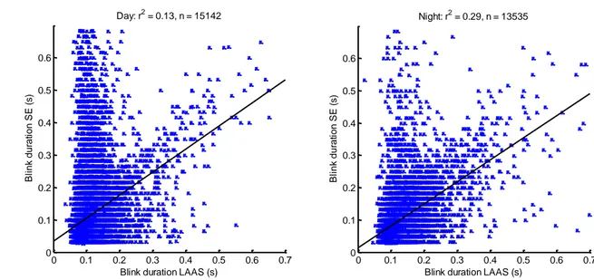
The linear regressions between the blink durations determined by LAAS and the blink durations determined by the camera system are shown in Figure 4. In the daytime sessions the correlation between the two systems is rather low (r2 = 0.13, n = 15142). In the night-time sessions the correlation is somewhat higher (r2 _{= 0.29, n = 13535), but it} is obvious that the two systems do not give similar results.

1050 1100 1150 1200 1250 1300 0 0.2 0.4 0.6 0.8 B lin k d u ra ti o n SE EOG 1180 1181 1182 1183 1184 1185 1186 1187 1188 1189 1190 -1.5 -1 -0.5 0 0.5 1 Subject 01-day Time (s) SE eyelid opening SE blinks EOG EOG/LAAS blinks Am pl itud e (a.u .)

(20)

Figure 4: Linear regression between the blink durations determined by LAAS and the blink durations determined by the camera system. Left: daytime sessions, right: night-time sessions. The discrete steps in data on the y-axis reflect the temporal resolution of the camera system. Data from the SleepEYE I field experiment.

Figure 5 shows mean blink duration obtained from the EOG and from the 1-camera system, respectively. For the EOG blinks, blink duration is higher in the night-time session than in the daytime session, which can be expected and is in line with previous research. However, for the 1-camera blinks the opposite can be seen, i.e. blink duration is higher during daytime. The result is about the same regardless of whether all blinks are included or only those that could be matched to EOG blinks. A similar result was found when the previous version of the camera system was evaluated (Fors, Ahlström et al. 2011). 0 0.1 0.2 0.3 0.4 0.5 0.6 0.7 0 0.1 0.2 0.3 0.4 0.5 0.6 Day: r2 = 0.13, n = 15142

Blink duration LAAS (s)

B li n k d u ra ti o n S E ( s) 0 0.1 0.2 0.3 0.4 0.5 0.6 0.7 0 0.1 0.2 0.3 0.4 0.5 0.6 Night: r2 = 0.29, n = 13535

Blink duration LAAS (s)

B li n k d u ra ti o n S E ( s)

(21)

Figure 5: Mean blink duration and standard deviation for all EOG and 1-camera (SE) blinks, respectively, and for matched blinks, i.e. blinks that were identified both in the EOG and in the 1-camera data. Data from the SleepEYE I field experiment.

In fourteen out of the 36 driving sessions the detection rate of the camera system was below 25%. The eye blink data and the video films from these sessions have been visually inspected in order to identify factors that can explain the low detection rate. In nine cases the driver is looking down at the speedometer a lot (about every ten seconds or more often), which possibly could explain the poor performance of the camera system. However, there are a lot of downward gazes also in some driving sessions with a higher detection rate, which means that downward gazes do not always result in poor performance. In three of the fourteen cases with low detection rate the driver was moving his head a lot, which caused noise and/or lost tracking. In the two remaining cases there were no particular factors identified that could explain the low detection rate.

3.1.2 euroFOT data

Blink data quality was mainly evaluated on data from the field experiment since EOG blinks were available in that data set. However, a brief quality check was done also on blink data in the euroFOT database. Only motorway trips were included (see also Section 3.3.2).

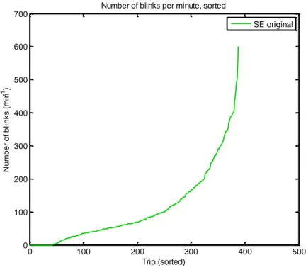
Figure 6 shows the average number of blinks per minute per trip from euroFOT, sorted in ascending order. The blink frequency is extremely high compared to what is

physiologically reasonable. As a comparison, the blink frequencies obtained by the 2-camera algorithms and by the EOG algorithm in the SleepEYE I field experiment are shown in Figure 7. The mean blink frequencies are 37 blinks/min (EOG) and 14 blinks/min (original camera algorithm), respectively. Note that the y axis scale is very different in Figure 6 and Figure 7.

EOG all EOG matched SE matched SE all 0 0.05 0.1 0.15 0.2 0.25 0.3 0.35 0.4 M e a n b li n k d u ra ti o n ( s) All blinks Day Night

(22)

Figure 6: Average number of blinks per minute for original camera data from euroFOT, sorted in ascending order.

Figure 7: Average number of blinks per minute for original camera data and for EOG data from the SleepEYE I field test, sorted in ascending order.

3.1.3 Conclusions

To summarize, factors that were found to be associated with low blink detection rate and/or incorrect blink duration were:

0 100 200 300 400 500 0 100 200 300 400 500 600 700

Number of blinks per minute, sorted

N u m b e r o f b li n ks (m in -1) Trip (sorted) SE original 0 5 10 15 20 25 30 35 40 0 10 20 30 40 50 60 70 80

Number of blinks per minute, sorted

Trip (sorted) N u m b e r o f b lin k s ( m in -1) EOG-LAAS SE original

(23)

 Downward gazes

 Sunlight

 Head movements

Furthermore, in euroFOT data the blink frequency was found to be far too high compared to what is physiologically reasonable and it was assumed that these data contained a lot of noise which led to false positives.

In conclusion, the evaluation of the improved version of the camera system showed that the system still missed a lot of blinks, was sensitive to noise and that there were too many incorrectly identified long blinks. The many missed blinks are unfavourable but they are perhaps not a considerable problem, as long as the blinks that are identified are correct and there are no systematic losses of data. However, the many incorrect long blinks will probably result in very poor performance when trying to identify sleepy driving in the FOT data. In addition, it was concluded that the unreasonably high blink frequency, i.e. the extremely many false positives found in euroFOT data, made it impossible to get any valid results from that dataset. Therefore, it was concluded that some post processing of the blink data was needed.

3.2 New blink detection algorithm

Based on the findings in the evaluation of the blink data quality a completely new blink detection algorithm was developed. This algorithm was implemented in Matlab (i.e. not in the camera system). Since the algorithm was intended to be used as a post processing algorithm for research purposes no optimization with respect to computation time had to be done, which allowed for more heavy/complex computations than what could be implemented in the (real-time) camera system.

3.2.1 Algorithm development

The detection of blink signals was implemented in three steps: a) the actual detection of possible blinks, b) a confirmation that the detection actually was a blink, and c)

measurement of the blink duration.

Detection, confirmation and measurement are made separately for left and right eye. If a blink is confirmed for both eyes at the same time the average of both durations will be used. After a blink is detected no other blink can be detected for a period of 0.15 seconds from the opening mid time.

For detection, the Gaze Quality signal is used. If it drops to near zero it is a strong indication that a blink has occurred.

For confirmation and estimation of blink duration, template matching using cross correlation is used. The blink template can be matched on two types of signals, each with its advantages and disadvantages:

 Gaze Quality: This signal is based on the iris detector and this feature is robust due to its elliptic appearance. It is not an accurate signal of the eye opening, meaning that the blink duration measurement would be poorer.

(24)

 Eyelid Opening: This feature is harder to detect and is more influenced by noise and artefacts, e.g. the frame of eyeglasses. On the other hand, it can give a more accurate estimation of the blink duration.

The selected signal is then pre-filtered through a median filter of length three in order to reduce the influence of short drop-outs and outliers.

For each blink detection, a falling flank template (Figure 8, left) is matched to the signal using cross correlation. The template is varied in size to correspond to different

velocities of the blink. If the match is above a given threshold the algorithm continues to check the rising flank. This is done in a similar manner, but the rising flank template (Figure 8, right) is altered to include a low value part to match the period of time when the eye stays closed. If this template then scores a correlation value over a given threshold, a blink is confirmed.

There are also some other criteria on the eyelid signal to decide whether it is a valid blink or not. These criteria were determined heuristically through testing on the dataset from the SleepEYE I field experiment. Many different criteria were tested and different versions were created. From these versions the best two candidates were selected for further testing, see Section 3.2.2.

Algorithm 1: The raw eyelid opening corresponding to the lowest value of the template

needs to be less than 3 mm, and the corresponding highest value more than 3 mm. The difference between these two needs to be at least 2 mm, and the difference from the end point of the falling flank to the start of the rising flank has to be less than 1 mm.

Algorithm 2: For the Gaze Quality signal the dependences are similar, but instead of an

eyelid opening in millimetres it is unit-less and divided by 10. So applying a 3 mm threshold on the eyelid opening corresponds to using 0.3 as a threshold on the gaze quality.

When a blink is confirmed the duration is determined by the distance between the closing midpoint and the opening midpoint. The midpoints are illustrated in Figure 8 as red circles.

3.2.2 Final selection of blink detection algorithm

The two most promising algorithms (algorithm 1 and algorithm 2 above) were compared according to a pre-defined evaluation plan:

Figure 8: The falling flank template (left) and the rising flank template (right). The red circles are the closing and opening midpoints, respectively.

(25)

For SleepEYE I field data

 Describe both algorithms when applied to this dataset: pros, cons, known problems, etc.

 Number of blinks detected: EOG, matched, camera-based per driving session

 Eye tracker availability (%)

 Detection rate: camera-based compared to EOG, matched compared to EOG o Per driving session

o Average day, average night

 Blink duration: EOG, camera-based

o Mean per driving session: day vs. night o Mean per driving session: alert vs. sleepy2 o Total mean: day vs. night

o Total mean: alert vs. sleepy

o Scatter plots of EOG vs. camera-based blink duration per driving session

For euroFOT data

Note: Include only motorway data and only data acquired with the last version of the eye tracker software.

 Describe both algorithms when applied to this dataset: pros, cons, known problems, etc.

 Descriptive plots:

o Distribution of blink duration (x-axis 0–1000 ms) o Blink duration per trip, sorted

o Blink duration per trip with standard deviation, sorted o Number of blinks per minute, sorted

o Number of blinks per minute with standard deviation, sorted o Blink duration and time of day

o Eye tracker availability (%)

 Include only trips with mean blink rate 5–75 blinks per min and generate the same descriptive plots:

o Distribution of blink duration (x-axis 0–1000 ms) o Blink duration per trip, sorted

o Blink duration per trip with standard deviation, sorted o Number of blinks per minute, sorted

o Number of blinks per minute with standard deviation, sorted o Blink duration and time of day

o Eye tracker availability (%)

 For trips with mean blink rate 5–75 blinks per minute, determine: o Number of trips

o Number of drivers o Total length in minutes

(26)

 For trips with mean blink rate 5–75 blinks per minute, check data:

o For trips (look at several trips, different drivers) with long mean blink duration (approx. > 0.15 s). Why is the blink duration long? True blinks? Systematic errors? Etc.

o For trips (look at several trips, different drivers) with a high blink rate (approx. 60–75 blinks per minute). Why is the blink duration high? True blinks? False detections because of noise? Etc.

o For trips (look at several trips, different drivers) with a low blink rate (approx. 5–10 blinks per minute). Why is the blink duration low? True blinks? Many misses? Any systematic misses?

The aim of the evaluation was to get enough information to be able to select the “best” algorithm. The criteria for the selection were:

 High blink duration accuracy,

 No systematic losses of long blinks,

 No systematic false positives (especially long blinks)

 A detection rate that is “good enough”.

The duration accuracy is of greater importance than the number of detected blinks, but with a very low detection rate (<10-20%) there is a high risk that we lose too much information.

A summary of the evaluation is shown in Table 1. In brief, algorithm 2 had a higher detection rate than algorithm 1, but algorithm 1 seemed to have a lower rate of false positives – particularly incorrectly detected long blinks – than algorithm 2. It was concluded that algorithm 1 had the best agreement with the selection criteria, and it was therefore chosen as the final blink detection algorithm. The performance of algorithm 1 is further described in next section.

Table 1: Summary of the evaluation of the two algorithms using SleepEYE 1 field data.

Parameter Algorithm 1 Algorithm 2

Detection rate day (%) 54 81

Detection rate night (%) 54 75

Detection rate day, matched (%) 46 57 Detection rate night, matched (%) 48 63 Mean blink duration per session,

number of sessions where blinkdurnight > blinkdurday

15 out of 18 9 out of 18 Mean blink duration per session,

number of sessions where blinkdursleepy > blinkduralert

(27)

3.3 Post processed blink data

Some descriptive data of the blinks detected by the final blink detection algorithm is presented in this section.

3.3.1 SleepEYE I field data

Figure 9 shows the number of blinks identified by LAAS and by the final blink

detection algorithm, i.e. post processed camera blinks and the number of post processed camera blinks that could be matched to EOG blinks. On average, the new camera detection algorithm detected 54% of the blinks detected by LAAS (day: 54%, night: 54%). This is considerably higher than the corresponding figure for the original camera algorithm, which was 39% (Section 3.1). Only one of the 36 driving sessions had a detection rate less than 20%.

Figure 9: Number of blinks detected by LAAS and by the final blink detection algorithm i.e. post processed camera blinks (Smart Eye), respectively, and the number of post processed camera blinks that could be matched to EOG blinks. Data from the SleepEYE I field experiment.

When looking at only matched blinks the average detection rate was 47% (day: 46%, night: 48%). In about 3/5 of the driving sessions more than 90% of the blinks could be matched to EOG blinks. This is somewhat lower than for the original camera blinks, where more than 90% of the blinks could be matched to EOG blinks in about 2/3 of the driving sessions.

In two sessions less than 60% of the post processed camera blinks could be matched to EOG blinks. For the original camera blinks, a low matching rate was found to be related to incorrect identification of long blinks. For the post processed camera blinks, the problem was related to a single individual for whom several problems were present: dazzling sunlight which makes the driver to squint, noisy signals and downward gazes.

1 2 3 5 7 8 9 10 11 12 13 14 15 16 17 18 19 20 0 1000 2000 3000 4000 5000 Day EOG-LAAS Matched Smart Eye 1 2 3 5 7 8 9 10 11 12 13 14 15 16 17 18 19 20 0 1000 2000 3000 4000 5000 Participant N u m b e r o f b li n ks Night EOG-LAAS Matched Smart Eye

(28)

The linear regressions between the blink durations determined by LAAS and the blink durations from the post processed camera data are shown in Figure 10. The correlations are lower for the post processed blinks than for the original blinks. In the daytime sessions r2_{is 0.016, n = 23322 (original: r}2 _{= 0.13, n = 15142). In the night-time}

sessions r2 is 0.06, n = 20852 (original: r2 = 0.29, n = 13535). The poor correspondence between LAAS and the post processed camera blinks with respect to blink duration is a disappointing result. However, a good thing is that the great amount of long blinks incorrectly identified by the camera system, mainly in the daytime sessions, is reduced by the post processing.

Figure 10: Linear regression between the EOG-LAAS blink durations and the blink durations from the final version of the post processed camera data (SE). Left: daytime sessions, right: night-time sessions. Data from the SleepEYE I field experiment.

The reduction of incorrectly identified long blinks is also reflected when comparing daytime blink duration with night-time blink duration, Figure 11. For the original camera data blink duration was lower at night than in the daytime sessions (Figure 5), but for the post processed camera data the opposite was found, which is the expected result and also in agreement with the LAAS blinks. When looking at individual driving sessions, the mean duration of LAAS blinks is higher at night than during the day for all 18 participants. For the post processed camera blinks the mean blink duration is higher at night than during the day for 15 out of the 18 participants.

0 0.2 0.4 0.6 0 0.1 0.2 0.3 0.4 0.5 0.6 Day. r2 = 0.016, n = 23322

Blink duration EOG-LAAS (s)

B li n k d u ra ti o n S E ( s) 0 0.2 0.4 0.6 0 0.1 0.2 0.3 0.4 0.5 0.6 Night. r2 = 0.060, n = 20852

Blink duration EOG-LAAS (s)

B li n k d u ra ti o n S E ( s)

(29)

Figure 11: Mean blink duration and standard deviation for all EOG and post processed camera (SE) blinks, respectively, and for matched blinks, i.e. blinks that were identified both in the EOG and in the post processed camera data. Grouped by driving session. Data from the SleepEYE I field experiment.

If blink durations are grouped into alert (KSS ≤ 7.5) and sleepy (KSS>7.5) the results look even more promising, Figure 12. When looking at individual driving sessions, the mean duration of LAAS blinks is higher when sleepy than when alert for all 15

participants that became sleepy. For the post processed camera blinks the mean blink duration is higher when sleepy than when alert for 14 out of the 15 participants.

EOG all EOG matched SE matched SE all 0 0.05 0.1 0.15 0.2 0.25 0.3 0.35 0.4 M e a n b li n k d u ra ti o n ( s) All blinks Day Night

(30)

Figure 12: Mean blink duration and standard deviation for all EOG and post processed camera (SE) blinks, respectively, and for matched blinks, i.e. blinks that were identified in both the EOG and in the post processed camera data. Grouped by KSS. Data from the SleepEYE I field experiment.

Figure 13 shows mean blink frequency per session, sorted by LAAS blink frequency in ascending order. For LAAS blinks the average blink duration is 37 blinks/min and it varies from 9 blinks/min to 73 blinks/min, while the blink duration of camera blinks range from 5 to 47 blinks/min with an average of 21 blinks/min. It is obvious that there is a lack of relationship between the two algorithms, with respect to blink frequency. However, blink frequency is not very interesting as a sleepiness indicator, so this might not be a problem. What also can be seen is that low blink frequencies may indicate a low detection rate. Figure 14 shows the relationship between detection rate and blink frequency for the post processed camera blinks. Blink frequency tends to increase with the detection rate, and it may thus be possible to use blink frequency as a quality criterion. Based on Figure 13 and Figure 14, it is suggested that a blink frequency of 5– 75 blinks/min should be regarded as valid.

EOG all EOG matched SE matched SE all 0 0.05 0.1 0.15 0.2 0.25 0.3 0.35 0.4 M e a n b li n k d u ra ti o n ( s) All blinks Alert Sleepy

(31)

Figure 13: Blink frequency per session, for LAAS and post processed camera blinks, sorted by LAAS blink frequency in ascending order. Data from the SleepEYE I field experiment.

Figure 14: Relationship between detection rate and blink frequency for the post processed camera blinks. Data from the SleepEYE I field experiment.

In conclusion, the final blink detection algorithm identifies about half of the blinks identified by LAAS. Blink duration shows a poor correspondence for individual blinks,

0 5 10 15 20 25 30 35 40 0 10 20 30 40 50 60 70 80

Session, sorted by LAAS blink frequency

B li n k fr e q u e n cy (b li n ks/ m in ) Blink frequency LAAS-EOG SE 0 10 20 30 40 50 0 20 40 60 80 100 120 140 D e te ct io n r a te ( % )

Blink frequency (blinks/min)

(32)

but it looks relatively good on the group level. No systematic errors have been

identified. It is suggested to use blink rate as a quality criterion, and to exclude driving sessions that have a blink rate outside the range of 5–75 blinks/min.

3.3.2 euroFOT data

All trips that had the latest version of the camera software and that were undertaken on motorways were filtered out from the euroFOT database. In total 2442 trips had the latest version of camera software, 715 of these trips did not have map data (thus it was not possible to calculate the type of road) and 192 trips did not have necessary signals to calculate the blink duration. Out of the remaining 1535 trips there were segments driven on motorway in 388 trips. Thus, in total 388 trips were filtered out, and from these trips only the motorway segments were included in the analysis. Eye tracking data from this subset of trips were run through the new blink detection algorithm (described in Section 3.2) and the results were summarized in the graphs below.

Figure 15 shows the average number of blinks per minute per trip. In 208 trips the blink frequency is very low (< 5 blinks/min), which probably indicates that the algorithm has problems detecting blinks. There are no trips that have an unreasonably high blink frequency, in contrast to the original blink data obtained from the camera software (Figure 6), which indicates that the new blink detection algorithm has a relatively low rate of false positives (i.e. noise classified as blinks).

Figure 15: Number of blinks/min per trip (blue), sorted by number of blinks/min. The red line corresponds to 5 blinks/min. Data from euroFOT.

In order to keep only the most reliable data for analysis all trips where the mean blink frequency was outside the interval 5–75 blinks/min were excluded, as suggested in

0 50 100 150 200 250 300 350 400 0 5 10 15 20 25 30

Number of blinks per minute, sorted Whole Trip - Trips on Motorways (388 Trips)

N u m b e r o f b lin k s ( m in -1) Trips

(33)

Section 3.3.1. For the remaining 180 trips the analysis was done only for the segments of the trips that were driven on motorways. Figure 16 and Figure 17 show descriptive data for the trips where the mean blink frequency was 5–75 blinks/min.

Figure 16 shows the distribution of blink duration. The shape of the distribution corresponds to what could be expected: most blinks are found in a relatively narrow duration interval, while a small amount of the blinks have a longer duration.

Figure 16: Distribution of blink duration from motorway segments. Trips where mean blink frequency is outside the interval of 5–75 blinks/min are excluded. Data from euroFOT.

Figure 17 shows mean blink duration and standard deviation per trip, sorted by blink duration. It is impossible to get any detailed information about the performance of the blink detection algorithm based on this figure, but what can be said is that there are no abnormalities identified in these data. However, it can be seen that there are very large variations in blink duration within the trips, but the reason for this is not known.

0 100 200 300 400 500 600 700 800 900 1000 0 1000 2000 3000 4000 5000 6000

Distribution of blink duration for the motorway segments

Blink duration [ms] N u m b e r o f b lin k s

(34)

Figure 17: Blink duration (mean and standard deviation) per trip (motorway only) for blink frequencies in the interval 5–75 blinks/min, sorted by blink duration. Data from euroFOT.

3.4 Summary and conclusions

The improved camera software was evaluated and it was found that it missed a lot of blinks, was sensitive to noise, and incorrectly classified downward gazes as long blinks. Therefore, it was concluded that some post processing of the blink data was needed in order to further improve blink data quality. This work was done in several steps and it finally ended up in a completely new blink detection algorithm which was implemented in Matlab (i.e. not in the camera software). The new algorithm had a better detection rate and a lower rate of false positives than the algorithm implemented in the camera system, and it was decided that this was the final algorithm that should be used in the project.

It was recommended that only trips with a mean blink frequency within the range 5–75 blinks/min should be included in the analyses, in order to minimize the number of trips where problems with the blink detection can be suspected.

0 20 40 60 80 100 120 140 160 180 -50 0 50 100 150 200 250 300

Blink duration with STD per trip sorted

Trips B lin k d u ra ti o n [ m s ]

(35)

4 Sleepiness indicators: selection, performance and analysis

The sleepiness detector developed in SleepEYE I, which was intended to be used in driving simulators, was based on the following sleepiness indicators:

 fracBlinks: fraction of blinks > 0.15 s, either from a camera-based system or from the electrooculogram (EOG)

 SDLP: standard deviation of lateral position

 KSSestSR: an estimated sleepiness level, based on the sleep/wake predictor (Åkerstedt, Folkard et al. 2004) and the KSS value (Åkerstedt & Gillberg 1990) reported by the driver immediately before the driving session

The indicators were calculated over a sliding window of 5 minutes. The detector aimed to classify whether the driver reported a KSS value of 8 or higher (actually higher than 7.5, since the sliding window approach may result in a value with decimals), where 8 corresponds to “sleepy and some effort to stay awake”. A set of decisions rules, in the form of a decision tree, was generated using the open source algorithm C5.03.

The selection of indicators was made with the simulator setting in mind. Since the project had a primary focus on camera-based indicators such indicators were naturally included in the development process. In particular blink related parameters were found to be very promising for sleepiness detection, based on the literature review that was carried out in the beginning of the project. In the literature review support was also found for using model based information (i.e. predictions of sleepiness level) and variations in lateral position as sleepiness indicators. In a previous study model based information, i.e. a sleep/wake predictor (SWP), alone was found to be able to detect sleepiness with a performance score of 0.78 (Sandberg, Åkerstedt et al. 2011). The SWP needs information about prior sleep, time awake and time of day, and since this

information usually is available in controlled experiments it was assumed to be a feasible indicator. Variation in lateral position is often used as a general measure of driving performance and it has been found to be related to sleepiness in several previous simulator studies (Liu, Hosking et al. 2009).

In the present project the aim was to adapt the sleepiness indicators described above to a field setting and ultimately to be applicable to FOT data.

4.1 SleepEYE I field data

4.1.1 Selection of indicators for field data

In a first step, the sleepiness indicators that were used in SleepEYE I were applied to data from the field experiment. For each single indicator the optimal threshold with respect to performance – defined as the mean of sensitivity and specificity – was calculated, as described in the SleepEYE I report (Fors, Ahlström et al. 2011). All indicators were calculated in time windows of 5 min with 1 min resolution. The target was to separate KSS > 7.5 from KSS ≤ 7.5.

The results were compared to the corresponding results from the driving simulator study.

3_{Available at www.rulequest.com}

(36)

Blink based indicators

Four variants of blink based indicators were assessed in SleepEYE I: mean blink duration, median blink duration, mean of 25% longest blinks and fraction of blinks longer than 0.15 s. The thresholds and performances of these indicators are shown in Table 2. As a comparison, the corresponding figures for the driving simulator data are included in the same table. It should be noted that the camera-based indicators for the field test are based on the new blink detection algorithm (post processed), while the simulator counterpart is based on the old camera software.

For the simulator test, the performances of the EOG-based and the camera-based indicators were similar, with a slight advantage for the camera-based indicators. For the field test, the performance of the EOG-based indicators was comparable to that of the simulator test, while the performance of the camera-based indicators was somewhat worse.

Table 2: Thresholds and performances of the blink based indicators. Note that the camera-based indicators from the simulator test originate from another algorithm than those from the field test.

Field Simulator

Measure Threshold Performance Threshold Performance

EOG mean blink duration 0.11 s 0.70 0.17 s 0.65 EOG median blink duration 0.11 s 0.72 0.13 s 0.64 EOG mean of 25% longest blinks 0.19 s 0.68 0.23 s 0.71 EOG fraction of blinks > 0.15 s 0.19 0.67 0.26 0.68 Camera mean blink duration 0.09 s 0.61 0.11 s 0.71 Camera median blink duration 0.10 s 0.61 0.10 s 0.70 Camera mean of 25% longest blinks 0.14 s 0.60 0.27 s 0.69 Camera fraction of blinks > 0.15 s 0.08 0.60 0.10 0.72

Lateral position variation

The threshold and performance of SDLP is shown in Table 3. The optimal threshold in the field test was identical to that in the simulator test. However, the performance was worse for the field test. Number of (unintentional) line crossings had a similar

performance in the field test as in the driving simulator test.

SDLP and number of line crossings were calculated in sliding time windows of 5 min with 1 min resolution (as all other indicators, as described in Section 4.1.1). SDLP was only calculated in time windows where the vehicle was in the right lane. Road segments where the lane tracker data was of poor quality or where the driver changed lane or drove in the left lane were excluded from the time windows. If more than 20% of the data in a time window had to be excluded due to the reasons above the entire time window was excluded from the analysis.

(37)

Table 3: Threshold and performance of SDLP in the field experiment and the simulator experiment, respectively.

Field Simulator

Std of lateral position (SDLP) 0.28 m 0.63 0.28 m 0.73 Number of line crossings (per 5 min) 0.09 0.67 0.90 0.69

Model based information

In SleepEYE I the SWP was used in combination with a simple model of how KSS changes with trip duration (time on task). By fitting a linear function to the KSS values reported every five minutes during the driving simulator sessions (averaged over all participants and conditions), and adding the slope of the function to the KSS value predicted by the SWP, the following model was obtained:

𝐾𝑆𝑆_{𝑒𝑠𝑡𝑆𝑊𝑃_𝑠𝑖𝑚} = 0.044𝑡 + 𝐾𝑆𝑆_𝑆𝑊𝑃.

where KSSSWP is the KSS value predicted by the SWP at the start of the driving session and t is time in minutes from the start of the driving session. The coefficient 0.044 is the slope of the linear function.

When developing the classifier in SleepEYE I KSSSWP was replaced by KSSSR, which is the self-reported KSS value just before the start of the driving session. The reason for doing that was that using KSSSWP resulted in a very poor performance for the validation data set, which included data from severely sleep deprived participants (which therefore did not correspond to the expected SWP pattern). In SleepEYE II no self-reported KSS values are available from the euroFOT data. Therefore, using KSSSR is not an option. On the other hand, in order to use KSSSWP information about the drivers’ sleep and wake up times is needed. Neither is this information available from the euroFOT data. A possible solution would be to estimate sleep and wake up times. A simple way of doing that is to assume that the drivers always go to bed at a certain time and that they always get up at a certain time. From here, this simplified SWP is denoted SSWP and the KSS values predicted from this model are denoted KSSSSWP. Using a similar approach as in SleepEYE I, KSS for field data can then be estimated according to:

𝐾𝑆𝑆𝑒𝑠𝑡𝑆𝑆𝑊𝑃 = 𝑘𝑡 + 𝐾𝑆𝑆𝑆𝑆𝑊𝑃,

where k is the change in KSS per minute, i.e. the slope of the curve. k was determined from the KSS curves from the field experiment, Figure 18. Separate functions were fitted to the daytime and the night-time data:

𝐾𝑆𝑆_𝑒𝑠𝑡_{𝑡𝑟𝑖𝑝𝑑𝑢𝑟𝐷𝑎𝑦} = 0.025𝑡 + 3.66

𝐾𝑆𝑆𝑒𝑠𝑡𝑡𝑟𝑖𝑝𝑑𝑢𝑟𝑁𝑖𝑔ℎ𝑡 = 0.027𝑡 + 6.00

Taking the average of the daytime and night-time slopes resulted in the following model:

(38)

In order to avoid invalid KSS values the following modification was done:

𝐾𝑆𝑆𝑒𝑠𝑡𝑆𝑆𝑊𝑃= {𝐾𝑆𝑆𝑒𝑠𝑡𝑆𝑆𝑊𝑃,_9, 𝑤ℎ𝑒𝑛 𝐾𝑆𝑆_{𝑤ℎ𝑒𝑛 𝐾𝑆𝑆}𝑒𝑠𝑡𝑆𝑆𝑊𝑃 ≤ 9 𝑒𝑠𝑡𝑆𝑆𝑊𝑃 > 9

When analysing data from the field experiment it is possible to use the original SWP instead of the simplified one, since sleep and wake up times are known.

Table 4 shows the thresholds and the performances of the two KSS estimates. In the SSWP, sleep and wake up times were assumed to be 06:30 and 22:30, respectively.

Table 4: Thresholds and performances for the KSS estimates when applied to data from the field experiment and from the simulator experiment.

Field Simulator

KSSestSWP 6.99 0.78 7.95 0.82

KSSestSSWP 6.83 0.78 - -

Figure 18: Mean KSS (blue) for all participants in the SleepEYE I field experiment and the linear functions that were fitted to the KSS curves (red). Left: daytime session, right: night-time session. A KSS values of 3 corresponds to "alert" while 8 corresponds to "sleepy, some effort to keep awake".

0 10 20 30 40 50 60 70 80 3 4 5 6 7 8 Day KSS

Trip duration (min)

KSS 0 10 20 30 40 50 60 70 80 3 4 5 6 7 8 Night KSS

Trip duration (min)

(39)

4.1.2 Discussion and recommendations

The camera-based indicators and SDLP had a worse performance when applied to field data than when applied to simulator data. There are several possible explanations for this fact. First, the driving simulator provides an experimental setting where things can be kept constant, e.g. traffic density, light conditions and road properties. Thus,

indicators that are sensitive to external non-constant factors, such as lateral position variation that is influenced by for example other traffic and road condition, can be expected to have a poor performance on real roads. Second, data quality is usually worse in real road tests compared to driving simulator tests, because of sensor failure, poor accuracy or noise. Another reason for the poor indicator performance in the field test is that the participants became less sleepy than in the driving simulator test, which is why the signs of sleepiness may be less pronounced. A related issue is that the perceived risk is greater on real roads, which may result in a difference in driving behaviour between the two tests.

Because of the poor performance, neither the camera-based blink indicators nor SDLP seem to be very feasible sleepiness indicators for field applications. It is a bit

unexpected that the camera blink indicators have such a poor performance, when almost all participants had a higher blink duration at night than during the day, and also a higher blink duration when sleepy than when alert (see Section 3.1.1). Perhaps there are still some problems with the blink detection that were not identified in the evaluation phase.

The EOG-based indicators had a better performance than the camera-based counterpart and they may thus have a greater potential to be used in field tests. The performance is however only moderate, so these indicators probably need to be combined with some other indicators in order to provide any useful results.

The number of (unintentional) line crossings had a somewhat better performance than SDLP and is thus probably the best driving related indicator. Similar to SDLP, the number of line crossings will be influenced by external factors, but probably not to the same extent as SDLP.

The KSS estimates showed relatively good performances, which were similar to the results from the simulator. It should, however, be noted that these indicators have not been evaluated on any other dataset, and that the assumed sleep and wake up times (which are needed for the calculation of KSSestSSWP) are very similar to the real sleep and wake up times in this dataset. Furthermore, when using KSSestSSWP individual variations are not taken into account at all. The indicator will only depend on time of day. KSSestSWP could perhaps be used in controlled tests where the participants’ sleep and wake up times are known.

In conclusion, KSSestSWP, number of line crossings, and EOG-based indicators are the most promising indicators for controlled field tests, but they are probably not very useful as individual indicators. Some data fusion and decision algorithms will be needed, and probably also additional indicators.

4.2 From SleepEYE field data to euroFOT data

4.2.1 Selection of indicators for euroFOT data

As demonstrated in the previous section, finding robust sleepiness indicators for field applications is very difficult and regardless of how the suggested indicators are selected