Revenue and creativity : Disentangling demand creating attributes in movies

J

I

B

S

R e v e n u e a n d c r e a t i v i t y

Disentangling demand creating attributes in movies

Master Thesis within ECONOMICS Author: Maria Eriksson

Tutors: Åke E. Andersson, Professor Erik Åsberg, Research Assistant Jönköping June 2008

Master thesis within Economics

Title: Revenue and demand: Disentangling demand creating attributes in movies

Author: Maria Eriksson

Tutors: Åke E. Andersson, Professor Erik Åsberg, Research Assistant Date: 2008-06-10

Keywords: Movie industry, hedonic price, economics of creativity JEL-codes: D12, L82, Z11.

Abstract

This paper’s aim is to outline a general model of the indicators of box office revenue for the top performing movies in history. The experience industry is different from most other in that the consumer good consist to a large extent of an emotion arousal. It thus lacks many of the features of normal consumption goods and the consumption experience is entirely based on previous experiences of similar kind.

Demand for experiences has two important influencers: income and leisure time. An increase in any of the two will increase demand for movie tickets. Production of experiences is based on a combination of an available set of attributes that are combined into goods in a monopolistic competition setting. It is assumed that quality is a function of educated labour.

These attributes were measured using hedonic price theory. This allows pricing of every unique attribute of movies individually, based on what the willingness to pay was in previous movies. Fifteen possible variables were tested in two models and the most important were shown to be actor, length, sequel, visual effects, age of actor, MPAA-rating and category (animations and dramas). All variables carried expected signs except the actor variables.

It is concluded that production companies are not entirely meeting the quality demands of the audience. Consumers are trying to reduce risk in consumption by referring to previous consumption experiences, and consumers have, according to the results, particularly strong positive experiences of movies with the kind of features that are significant in the test.

Table of Contents

1

Introduction... 1

1.1  Background ...1 

1.1.1  Previous research...2 

1.2  Aim and purpose ...3 

1.3  Outline ...3 

2

The market for experiences ... 4

2.1  Demand for experiences – the importance of leisure time and income 4  2.2  Determinants of creative output...7 

2.2.1  The Economics of talent ...9 

2.3  Hedonic consumption and pricing...10 

2.4  Measuring the value of creative goods ...12 

3

Empirics ... 13

3.1  Data set and variables...13 

3.1.1  Independent variables ...14 

3.2  Model outline ...18 

3.3  Results ...18 

4

Model interpretation ... 22

4.1  The unique variables ...22 

4.2  Beyond the model...24 

5

Conclusions ... 26

References... 27

1

Introduction

The movie industry is an industry of extremes. It deals with illusions and fairy-tales on a daily basis and the spectacular news about movie stars, box office ratings, sky-high budgets and record breakers do seem surreal sometimes. The business is rather extreme from a geo-economic viewpoint as well. Its geographical concentration is exceptionally high with only a few locations producing almost all movies for the international market.

This production of movies is associated with high uncertainty. Despite years of trying to forecast what factors will make a movie popular there is yet no formula for success. Productions including highly rated movie stars, having large openings and advanced marketing systems are common strategies but no profitability insurance. As the structure of the business has changed to judge every project’s success probability, instead of as a part of a portfolio, risk management has been reduced to a process of advanced guesswork for every film.

The high production risk is due to the difficulty of estimating box office demand, which is very hard to forecast due to every movie’s uniqueness. Since the particular characteristic in consumption of movies is its irrevocability, purchasing a movie ticket involves a large risk for consumers too. The expenditure is based on their expectations about the good, but whether these were realized or not is only possible to find out after the movie ticket has been consumed when the expenditure is irrevocable. Consumers’ utility thus depends on the level of their expectations and to what extent the movie satisfied them. The goal of most film-makers is thus to create a movie that communicate high expectations to consumers in order to increase willingness to pay, popularity and life time of the creation.

1.1 Background

The movie industry is a rather young business, originating in France after Edison’s first initial development of the recording camera in the 1890’s. When the importance of the American west coast grew during the 1920’s the creative region of Hollywood emerged and has since then been the global centre of movie production. The industry faced a financial obstacle when the Depression hit at the same time as the new expensive sound equipment became necessary: only a few major distribution companies survived and these have since then dominated the market. An antitrust lawsuit in 1948 further changed the industry drastically: from controlling the whole distribution through direct cinema ownership they were now forced to compete for screens on more and more independent cinemas (Vogel, 2004).

The industry’s development has after that followed the development of its most important foundations: technology, capital and distribution systems. As technology was growing advanced more and more complex projects have been made possible. The sophistication of the financial market has allowed for more efficient financing of movies and as distribution chains with large theatre chains evolved more viewers became potential buyers. Producing and distributing motion-pictures has evolved to a diverse industry with a complex system of economic cooperation. It is however the handful number of companies with presence in both production and distribution that are the most influential. These finance, produce and distribute movies in their own studios, but have during the last decenniums also increased cooperation with independent producers and thus decreased the high dependency on studios that earlier prevailed (Vogel 2004).

This market strategy is taking its form on the global market as well. Concerning the American movie industry the same major companies are dominating the global market and the American domestic (McChesney, 1999). International competition is however challenging, although the movie industries of Bollywood and Hong Kong are so far not exercising any major influence on geographic areas outside their own territory, their strength on national markets is impressive (Bordwell, 2000). Overall, all three geographic areas of movie production is experiencing a growing market. Although competitive, the global market’s potential is substantial due to its rapid growth, as can be seen in figure 1-1. Almost the whole growth in revenue during 2001-2007 was international gains.

Figure 1-1: Global and American development of box office revenue 2001-2007 for U.S. produced films

The industry’s main task today is to master the uncertainty. The problem is to understand consumers’ expectations. As the consumers naturally have no experience of the actual alternatives available, they have to rely on previous experiences of movie attributes. Positive experiences of one set of attributes, for example a drama-thriller with Tom Cruise directed by Steven Spielberg could be influencing future willingness to pay for movies with similar features. To what extent are people willing to pay to see a movie associated with celebrities and certain features? What attributes are determining a movie’s success? This is valuable information for producers, distributors and perhaps most of all financers in the movie industry.

1.1.1 Previous research

The previous research in the field is extensive. There is especially a large amount of empirics from a marketing perspective. Any general results have however not been concluded in neither marketing nor economics. The results on what determines box office revenue are at best inconclusive. De Vany (2004) has propagated that this is the normal structure of the industry: it is characterized by an atmosphere of “no one knows anything” and factors such as stardom and budget are so dynamically complex they appear to be statistically chaotic.

Yet some researchers manage to find relationships using limited data sets. The least controversial variable seems to be budget where all empirics support a positive relationship, yet not without large variances (De Vany (2004), Terry et.al. (2005), Basuroy et.al. (2003), Ravid (1999), Simonton (2005)). Other significant determinants have proven to be sequels, MPAA-rating (the age allowance ratings issued by the American Motion Picture Assosication), opening season, number of opening screens and critical reviews.

The main controversy lies in whether star power is influencing revenue or not. Much of the variation is due to the changing structure of the industry, during the studio area when stars were employed by production companies the dependency on individual actors were larger. Most articles fail to find a significant relationship between indicators such as star quality and box office revenues and many of the rather rare investigations that show a positive correlation have been using data from the studio era (for an extensive summary, see Albert, (1998)). Albert (1998) however, is successful in showing that movie stars act as markers of certain movie types which is influential in consumers’ future behaviour.

Many other movie features that generate expectancies are missing in the research: the impact of category, spectacularity, length, original manuscript and personal features of actors like age has not been uncovered. Global empirics are also missing although there is a growing importance of this kind of research from an international perspective.

1.2 Aim and purpose

The aim is to uncover what movie attributes are influencing global audiences’ willingness to pay based on a dataset consisting of the most internationally successful movies. Through hedonic price theory, movies’ attractive characteristics can be separated from each other and valued in order to determine what movies will be successful.

The purpose of this paper is to outline through a hedonic price theory setting what movie attributes in terms of contributing professionals and creative attributes is increasing audiences’ willingness to pay for movie tickets.

1.3 Outline

Section 2 will outline a theoretical market setting for experiences, starting with demand creation of experiences followed by production models of creativity and willingness to pay. In Section 3 the empirical model and the data set is presented along with the results of the econometric testing.

2

The market for experiences

An experience is different from many other goods in that it is an inherently personal adventure: it exists only in the mind of the consumer and is formed as a reaction on an emotional, physical or intellectual level. As an experience is an interaction between a staged event and an individual’s state of mind, it follows from this definition that experiences are highly individual and that not two spectators or participants of an experience will judge the event equally (Pine & Gilmore, 1998).

The main economic characteristic of experience goods and services is its intangibility. As an experience is an emotional reaction within the consumer it cannot be evaluated in the same sense that most other goods are. The consumer cannot evaluate his utility of the good using previous experiences of the good, nor can he return it if it did not meet his expectations. If the good indeed succeeded in meeting the expectations, price decreases will not necessarily mean further purchases in the future. Neither will there be any hoarding as experiences cannot be stored for later consumption. As the consumer cannot use collected knowledge about the good in the evaluation process he has to use only expected costs and benefits in the decision to spend or not (Andersson & Andersson, 1998).

2.1 Demand for experiences – the importance of leisure time

and income

This section will outline a model of consumption determinants of experiences. The two most important factors are the amount of leisure time and income. But by definition if one of them increases the other will decrease: they are at first sight substitutes to each other. This is not entirely true: above a certain wage level the total income is high enough to offset the incentive to work more when income increases: people are earning enough to afford leisure time. The following model (adopted from Brems (1968)) outlines the importance of both effects for demand of experiences:

Let the individual maximize a utility function: ) , (W l U

U = (2-1)

where W equals wage income per annum and l hours of leisure per annum. By definition, income is the product of hours worked, x, and the rate of income, w:

wx

W = (2-2)

where the time available for working is restricted by the total time available, h: l

x

h= + (2-3)

If the above functions then are combined it is possible to state the time budget constraint: 1 + ⎟ ⎠ ⎞ ⎜ ⎝ ⎛ = w W h (2-4)

If the utility function then takes the form of a constant-elasticity-substitution type, the maximization problem becomes:

subject to ρ ρ ρ 1/ ) ( − + − − = AW Bl MaxU ⎟+1 ⎠ ⎞ ⎜ ⎝ ⎛ = w W h (2-5)

Where the substitution parameter -1 < ρ< 1, and A and B are parameters of constant-elasticity-substitution functions. If the maximization problem then is set as a function of x only, differentiated with respect to x and solved for x, one will get the following solution:

) 1 /( 1 1 ρ ρ + ⎟ ⎠ ⎞ ⎜ ⎝ ⎛ + = w A B h x (2-6)

Supply of working hours is thus a function of total availability of hours, wage rate and the substitution parameter ρ. Why this function is of importance to demand for experiences can be understood when the above function is derived for wage rate:

h w A B w A B w x ) 1 /( 1 ) 1 /( 1 1 1 1 ρ ρ ρ ρ ρ + + ⎟ ⎠ ⎞ ⎜ ⎝ ⎛ + ⎟ ⎠ ⎞ ⎜ ⎝ ⎛ + = ∂ ∂ (2-7)

What matters in this function is whether ρ is positive or negative: the partial derivate will have the opposite sign to ρ, and the function will be positive if -1 < ρ< 0. In this case leisure time and working time are close substitutes so that when the price of an hour, w, is increasing, the Hicksian substitution effect outweighs the income effect so that the households will work more when income increases.

If ρ > 0 on the other hand, income and leisure are not easily substitutable for each other. In this situation the income effect outweighs the substitution effect so that the increase in income fails to induce more working. Leisure time will increase.

Individuals will then divide time between leisure and work in order to achieve the highest level of utility, depending on the substitution parameter value, the wage level and the corresponding leisure time. Disposable income and time is therefore the most influential determinants of entertainment demand.

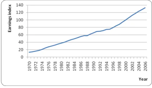
In Figure 2-1 and 2-2 the development of the OECD countries’ average earnings and leisure time is shown. The strong pattern of increased earnings and decreased work time is indicating that OECD’s member countries has gained wealth since 1970 which should have lead to a growing demand for movie theatre tickets.

Figure 2-1: Average hourly earnings index, 2000=100 for OECD countries, 1970-2006

Source: data from OECD, author’s own illustration.

Figure 2-2: Average yearly hours of working in OECD countries, 1970-2006.

Note: Data for South Korea is missing.

Source: data from OECD, author’s own illustration.

It follows from this reasoning that low-income groups can in some situations have a higher propensity to consume because the low income is not enough incentive to work, and they will consequentially have much leisure time. This effect is hypothetically large in groups such as teenagers, elderly and unemployed. Hill (1985) finds support of this that American adults’ active leisure time (sports activities, cultural activities and hobbies) reaches top levels in the age groups 18-24 and 65+. The findings also show that unemployed spend more time on active leisure than both part-time and full-time workers although their income is lower. The distribution of American box office revenue according to age group is seen in Figure 2-3. No age group is outstanding and the only major change during the time period is the growth of the group 40-49.

Figure 2-3: Movie revenue according to age of visitor 1985-2002 in U.S.

Source: MPAA as shown in Vogel (2004).

This time and income distribution in the population is also a possible explanation to why the income elasticity of demand for leisure and entertainment is unexpectedly low in many empirical tests. Demand for such activities grows faster than the level of income and is thus elastic with a value above 1. Yet values very close to one or below is rather common (see for example Andersson & Andersson (2006)).

Another concept influencing demand is noted by Caves (2000): the importance of putting consumption of creative goods in its social context. Although it poses as an irrational economic behaviour, consumers are influenced by their social situation in their decision process. The consumer’s company on a night out for example will affect the perception of the experience through pointing out new attributes or perhaps exercising unintended group pressure. The word-of-mouth effect is also important in this context: what consumers buy tend to depend on what they observe and learn other people are buying. Demand as a function of the social context is therefore an exponential function.

2.2 Determinants of creative output

This section will discuss a model for production inputs and allocation theory of creative goods. Price of goods produced in monopoly settings and in monopolistic competition is a function of a number of demand determining factors:

) , , (q m L_u p p= (2-8)

where p equals price of the final product, q quantity, m marketing and Lu educated

(creative) labour such as directors, producers, actors, make-up artists, composers, editors, writers and technicians (model adopted from Andersson & Andersson (2006)). Quantity is assumed to have a negative effect on price as the more units sold the lower price will have to be offered in order to meet lower reservation prices (assuming a downward sloping demand curve). Marketing is one of two ways to increase demand by shifting the demand curve to create a higher willingness to pay. The second, quality, is in turn a function of the

amount of educated personnel used as an input in production. Lu is an input to marketing

as well, and qualified personnel therefore act bidirectionally through both quality level and sophistication of marketing. How the willingness to pay is influenced by these attributes can be determined through their respective price elasticities:

qp q p p q _ε = ∂ ∂ * (2-9) mp m p p m _ε = ∂ ∂ * (2-10) p L u u u L p L _ε = ∂ ∂ * (2-11)

A high elasticity value indicates that the attribute does not have much influence on price and willingness to pay: a very high increase in the attribute will not cause demand, and therefore price, to increase. These price tools should therefore not be influential in the production decision process. A very low elasticity value on the other hand denotes a feature that is valuable to the consumer and is influencing willingness to pay very much. For movies it is expected that the first of the elasticities is of lesser importance: there is no significant price differences between movies released to large audiences compared to smaller productions. The last two however, i.e. the two that are functions of educated labour, are hypothesised to be important for demand creation.

The firm’s revenue function in this setting is a compound of the attributes determining demand; quality and quantity, and the cost function is associated with the costs of these inputs: ) ( * ) (Lu q Lr p R= (2-12) r r u uL w L w C = + (2-13)

where p(Lu) is the function of quality inputs, q(Lr) is the quantity which is assumed to be a

function of uneducated or unspecified labour and wu and wr are wage levels where wu > wr.

Capital in this model is assumed to be proportionate to either Lu or Lr and is therefore not

included in the formal writing. The only production inputs are educated and uneducated labour, and the only production costs are wages. The profit function is then defined:

r r u u r u q L w L w L L p V = ( ) ( )− − (2-14)

where V equals profit. Optimal allocation of creative inputs is derived through the marginal conditions of revenue and cost. The marginal revenue and cost functions of Lu

and Lr are given by:

q w L p L R MR u u u L_u = ∂ ∂ = ∂ ∂ = (2-15) u u L w L C MC u ∂ = ∂ = (2-16)

where q is determined through optimising the value of Lr inputs: r u L L q L p MR r ∂ ∂ = ( )* (2-17) r r L L r ∂ w C MC = ∂ = (2-18)

compared to smaller firms and it is therefore possible for large firms to make both more

increased, but their payoffs are justified only in those cases where they succeed in ommunicating the selling elements of the movies (Caves 2000).

man inputs: a close

rtist has to put equal amounts of conomy allows a few sellers to serve the whole market.

As can be seen, the optimal level of educated personnel depends on the level of q, quantity inputs, i.e. the level of uneducated personnel. Because the change in marginal cost of Lu is a

function of q there are economies of scale to be gained in production. The larger a company is the less sensitive it will be to price changes in Lu since q will be very high. The

main global producers in the movie industry therefore have a strong production advantage compared to smaller competitors. To them quality is cheaper due to a lower relative price and more sophisticated movies in terms of creativity.

The choice of personnel is based on a preference set which in turn is based on expectations about the ability to add to profits. The goal is to communicate value to the audience, a task not merely the actors’ but involve all creative personnel. The labour is differentiated both horizontally and vertically: how does he/she compare to other similar and how is he/she in relation to others above and below on the list of asking prices? This in turn gives bargaining power to top performers in their field, and as a good “match” between the creative inputs seems to create large economic synergies. As a consequence the bargaining power of late contracted is increasing as the relative importance of their participation has c

2.2.1 The Economics of talent

The reward system for these chosen persons is quite unlike most other. Only a few individuals have the privilege of earning money on their creative performances although their talent is not in proportion to their often excessive incomes. Rosen (1981) came with the ‘Superstar Phenomenon’ up with a theory to why certain individuals can earn so much more income with only minor differences in talent and where growth of the market size is completely captured by existing participants. According to Rosen, there are two key elements necessary to observe these patterns in a market for hu

connection between rewards and the size of one’s own market along with a tendency for skewness of both market size and reward to the top talented people.

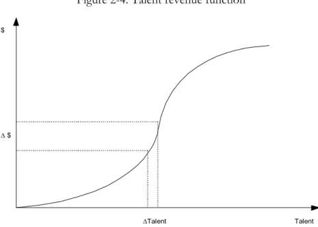
The explanation to the skewed income is found in the convexity of the sellers’ revenue function, which is dependent on talent, or quality. Convexity has the implication that the longer to the right of the curve very small differences in talent give very large changes to income as seen in Figure 2-4. This property is a result of imperfect substitution between sellers’ goods: highly talented performances cannot easily be replaced by a larger quantity of lower talented. Later the curve will flatten out when there is no longer use for extra units of talent. The high concentration of performers is explained by technology which allows for marginal cost of a performance to be virtually zero. The a

effort into a production whether it is ten or ten thousand people watching. This scale e

Figure 2-4: Talent revenue function

$

Talent ∆ $

mmonly used well-known movie stars in order to minimize search ost.

∆Talent

Chung and Cox (1998 & 1994) found using a stochastic model that the superstar phenomenon was an appropriate model for explaining the distribution of appearances in movies for a set of actors. The distribution was found to follow a Yule distribution and was thus consistent with Rosen’s theory. The authors defined consumers as casting directors and found that they co

c

2.3 Hedonic consumption and pricing

The particular features of consumption that are arousing emotions in the consumer are known as hedonic. Many goods are emotion creating by nature, experiences for example, but attaching an emotion to a product is also a very efficient marketing strategy for value creation. Experience goods like movies are an example of products where hedonism is decisive for success: the very idea with selling a movie is to engage the audience. Hirschman & Holbrook (1982) describe hedonic consumption as “those facets of consumer behaviour that relate to the multi-sensory, fantasy and emotive aspects of one’s experience with products” (p. 92) where multi-sensory refers to the experience processed through the senses: taste, sound, visuality, scent and tactility. The sensory experience in turn creates an image based on history or fantasy: a memory of a previous experience of something or something missing a relation to reality. In addition to these images there will be an arousal of emotions within the consumer. In the light of hedonic consumption the “objective entity” is of less importance in favour of their value as “subjective symbols”. What the good represents is more important than what it actually is.

The traditional view of utility-derived consumption is in this sense not denied but rather deepened, by recognizing the many sensory channels utility can originate from. Hedonic consumption can through this deepened definition also explain the behaviour of consuming products the buyer knows will make him/her sad. In traditional consumption

theory the consumer will only buy if the utility gained from the product is larger than the utility loss of decreasing wealth. This will not be the case of particularly painful experiences, for example a parent engaged in a custody fight watching Kramer vs. Kramer. But through hedonic consumption this behaviour can be explained through a particularly strong emotion arousal which creates value to the consumer. Higgins (2006) proposes that this phenomenon is in some situations due to an effect called “motivational force experience” arising simultaneously with the hedonic attributes of consumption. This force of motivation compensates for negative emotions through thoughts like “I don’t like this but it is good for me” or “this is the right thing to do” or even in the case of movies “everyone else is doing it”. As an effect of this duality a very common marketing measure initiated by Babin, Darden and Griffin (1994) is therefore to represent consumption value on a

two-than in equilibrium. The determinance of

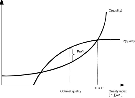
uality levels beyond the point where C=P firms will run deficits. The optimal quality level is instead where the slopes of C and P are tangent and where profit will be maximised.

dimensional scale representing pure utility and the hedonic experience (see for example Chadhuri & Holbrook (2001) and Sweeney & Soutar (2001)).

Hedonic pricing is a valuation method of differentiated goods. If goods are assumed to have the different utility-bearing features described above, they can through separation be valued. The prices of these attributes, the hedonic prices, are revealed through economic choices of consumers and producers. The characteristics can be seen in a spatial equilibrium setting through a vector of coordinates z = (z1, z2, z3, ... , zn) where zi is representing the amount of each characteristic in each good. As consumers and producers choose between bundles of characteristics a multidimensional equilibrium over the characteristics evolve. As no producers add any mark-up and treat the prices as parametric to their decisions, and as both consumers and producers are acting to maximise utility no economic actors will be able to be better off

equilibrium is similar to that in a simple competitive environment: through consumer preferences and producer costs (Rosen, 1974).

The situation is shown in Figure 2-5. Hedonic price is a function of zi weighted by wi and is an upward sloping yet diminishing curve. Initially consumers are prepared to pay very much more for slightly higher quality, but at high levels the use of additional units of quality is limited and therefore less valuable. The cost function of quality is an inverted revenue curve: upward sloping and increasing. The curvature of the cost and revenue functions are indicating that an optimal quality level is not the highest possible. For q

Figure 2-5: Hedonic price and optimal quality of goods Hedonic price Quality index ( = ∑w_iz_i ) C(quality) P(quality) Optimal quality Profit C = P

Hedonic pricing has been applied on several differentiated markets like cars and housing, but most markets can be considered since very few product categories include identical products (Andersson & Andersson, 2006). In the field of movie economics, the theory has previously been used to uncover preferences in a wide range of areas, for example movie theatre demand (Davis 2001) and mood experiences of movie consumption (Eliashberg & Sawhney, 1994).

2.4 Measuring the value of creative goods

Measuring art in monetary terms is a well-debated issue between social-scientists and economists. Economists have the habit to assume rational decision-making although creative goods are very often quite abnormal. The difficulty is often to measure quality, most people would probably agree on the notion that there is not necessarily a connection between revenue and quality. Some have instead tried to estimate quality through reviews and awards (see for example Bagella & Becchetti, 1999 and Ginsburgh & Weyers, 1999). Frey (2001) does however recognise that there is more than one dimension of demand for creative goods: it is not only the number of visitors to a cultural event that is important but also their intensity with which it is enjoyed. Willingness to pay is thus not only a measure of visitors but also of experience intensity and choice.

An important concept not to be forgotten in this debate and which is highly relevant to the movie industry is taste. Differences in taste have for a long time been left unexplained by economists and it is only recently that the topic has been addressed (Caves, 2000). This paper does not try to measure quality in movies but rather taste or preferences.

3

Empirics

This section will introduce the data set and the chosen variables along with a presentation of the models and the regression results.

3.1 Data set and variables

The data set is collected from the Internet Movie Database (retrieved February 2008) and The Numbers1 _{(retrieved April 2008) and consists of the 162 top revenue generating} movies on the world market. Complementary data of content ratings was retrieved from the Motion Pictures Association America (MPAA)2_{. As the data is continuously updated} there will be a bias towards older movies that are no longer generating revenue (5 movies on the list were still running on theatres at the time of data retrieval). The top fifteen movies of the sample are shown in Table 3-1.

The relative importance of actors has been determined through first-billed lists. A top placement on the list may not mean most minutes of exposure in the movie, but it is natural to assume a high rate of audience association between the movie and the first paid actor.3

Table 3-1: Top 15 box office revenue movies all times in the global market

Rank Title Box office revenue ($) Year of release

1 Titanic 1 835 300 000 1997

2 The Lord of the Rings: The Return of the King 1 129 219 252 2003 3 Pirates of the Caribbean: Dead Man's Chest 1 060 332 628 2006 4 Harry Potter and the Sorcerer's Stone 968 657 891 2001 5 Pirates of the Caribbean: At World's End 958 404 152 2007 6 Harry Potter and the Order of the Phoenix 937 000 866 2007 7 Star Wars: Episode I - The Phantom Menace 922 379 000 1999 8 The Lord of the Rings: The Two Towers 921 600 000 2002

9 Jurassic Park 919 700 000 1993

10 Harry Potter and the Goblet of Fire 892 194 397 2005

11 Spider-Man 3 885 430 303 2007

12 Shrek 2 880 871 036 2004

13 Harry Potter and the Chamber of Secrets 866 300 000 2002

14 Finding Nemo 865 000 000 2003

15 The Lord of the Rings: The Fellowship of the

Ring 860 700 000 2001

Source: IMDB.com.

The dependent variable, box office revenue, is an estimation of theatrical box office receipts sold in all countries where the movie was available on cinema.

1 _{http://www.IMDB.com/ and http://www.the-numbers.com/} 2 _{http://www.mpaa.org/Filmratings.asp}

3 _{In the trilogies Lord of the Ring and The Matrix there is no pay list available. The relative importance of actors} in these movies has instead been determined through individual exposure on marketing posters.

The reader should be aware that all movies in the sample can be considered successful in most general terms. Monetary measurements of success are often outlined through a threshold value in the range of $200-250m whereas the lowest revenue generated in this sample is $311m.

The distribution of revenue according to rank follows an interesting pattern, as seen below in Figure 3-1. The further down the ranking the smaller is the variation. The higher the revenue goals are the more difficult they seem to be to reach: the number of movies to the right of the scale is substantially more than to the left for the top placements. Only three movies have succeeded in exceeding $1 billion but the number of attempts is many. The purpose of the empirical tests is to find what variables that can possible create such a pattern.

Figure 3-1: Revenue and logged rank of the 325 revenue top movies

Titanic 0 200 400 600 800 1000 1200 1400 1600 1800 2000 -0,5 0 0,5 1 1,5 2 2,5 3 M ill io n s Logged rank R even u e

Source: data from Internet Movie Database, author’s own illustration.

3.1.1 Independent variables

Year: There are two important reasons to include time as a determining factor of revenue:

(1) the data is not inflation adjusted and will therefore be positively correlated with time and (2) the global market for movies is constantly growing. If this variable would not be included there would be a strong bias towards newer movies at the expense of classics that were market leading during the days of their releases.

Input of professionals: The importance of creative inputs of both exposed and less

relationship with revenue. There are several approaches to measuring importance, using for example notations such as ‘talent’, ‘successfulness’ or ‘fame’, and most of them will be tested here for both actors and directors. These notations are believed to express approximately the same trend in the dataset and will therefore be used as substitutes in the empirical testing. Only the most suitable will then be analyzed.

- Talent: the most common method of measuring talent is to use the industry’s own reward system, the Oscars. Two dummy variables will be included expressing any previous Oscars received by the lead actor and the director in their respective fields. - Successfulness: this variable may not to everyone denote monetary wealth, but to ease empirical testing of this very subjective notation it is assumed most other measurements of success (respect, wisdom, professional freedom) are correlated with wealth. This is thus a measurement of the revenue generated by previous movies that the professional has played a part in. For actors it is a role that earned him/her salary and for directors it is previous directions.4

- Fame: This variable could be quite different from the two above. Intra-industry crossovers by performers such as actors, musicians and models are quite common and this variable thus recognizes the fame gained in other creative fields. This variable will only be tested for the three leading actors as it is assumed that the director’s name is not generally known to the public. The variable will be measured through Google hits (as of February 2008) which is a measurement indifferent to what fields the person is famous for.

Age of actors: This is a hypothesis that will be tested alongside the above, and is based on

audience identification. It is a method of trying to outline what part of the market the movie is trying to appeal to. Very young actors for example, tend to star in movies targeted to an audience in about the same age. Similar patterns can be found in other age categories concerning television shows and there is no reason to believe that movies are different from television (Harwood 1997). A significant value of children as actors in the leading role is an indication that this audience has a high willingness to pay for movies. The leading actor’s age is divided into four age groups: >18, 18-29, 30-49 and 49< and will be tested through dummies.

Sequel: Sequels are very important in the movie industry, in the sample used for this paper

seven out of the top ten movies are sequels (see Table 3-1). Theoretically, the more alike two movies are the larger should the predicting power of the second movie’s revenue be. But the sequel also has to take into account that the audience now has a very specific expectation set, something that is both valuable and dangerous.

4 _{The success variable for actors does not account for variations in importance of the role, but as the} distribution of different important roles should be normal (the number of well-known stars in less successful movies is expected to be the same as unknown actors in highly profitable movies) this should not pose as a problem. There is however a problem of simultaneous releases, some movies are released while there is still another movie running on screens that have the same actor or director. This will result in too high previous revenue figures for the second movie as the first has not yet earned all that is recorded. The problem is more frequent with actors since they have an important part in only one stage of production. Orlando Bloom did for example have a busy autumn in 2003 as the blockbusters ‘Pirates of the Caribbean: The Curse of the Black Pearl’ and ‘Lord of the Rings: The Return of the King’ had overlapping release dates all over the world.

Original manuscript: If the movie builds upon a creative work already known to

audiences this will affect the expectations of the movie and thus willingness to pay. Original manuscript is a dummy with the value 1 if the movie’s manuscript is based on a book, comic or a character known from any kind of literature (the James Bond movies are an example of this latter category).

MPAA rating: MPAA’s rating system is a voluntary measure of the movie content based

on level of violence, sex and nudity, improper language, drugs and other material considered inappropriate for different age groups. The rating is not internationally recognized and there is no general tendency for other national censorship institutions to follow MPAA’s. This category should instead be considered as an indication to what audience the movie is trying to target. The lower ratings G and PG imply a family movie and should be able to generate high levels of revenue since the hypothetical audience is larger. Since the distribution of G and PG-rated movies in the true population5_{, is} substantially lower than majority (only 17 percent) the strategy is obviously not to target the largest audience possible. This is further confirmed by the rate of R-rated movies, in the population this number is 46 percent, dominating all other ratings. Reaching the lower levels of rating is also quite a challenge; it takes only one of the harsher sexually oriented words or any sexual nudity for the movie to be raised to PG-13. The sample distribution is very different from the population, see Table 3-2. In this sample it seems that there is a positive effect between the size of the hypothetical audience and revenue. The dummy variables for G/PG and perhaps PG-13 are therefore expected to be positively correlated with revenue.

Table 3-2: MPAA ratings and sample distribution

Rating Explanation Sample distribution

G General audiences allowed. All ages admitted. 7% PG Parental guidance suggested. Some material may not be suitable for

children. 25%

PG-13 Parents strongly cautioned. Some material may be inappropriate for

children under 13. 50%

R Restricted. Under 17 requires accompanying parent or adult guardian. 17%

NC-17 No one 17 and under is admitted. 0%

Source: Movie Picture Association America

Category: The category a movie belongs to is important to revenue for many reasons. It is

perhaps difficult to argue that one kind of movies is “better” than another and therefore generating more revenue, but some movies are for example better suitable for cinematic view on large, high quality screens and sophisticated audio systems. In these kinds of movies, action movies for example, the technological setting is exploited to a higher degree than other movies which may affect the audience’s willingness to pay for the cinema experience. Some categories of movies may target a specific demographic group that have a higher willingness to pay than other categories. The distribution of categories in the movie sample reveals a dominance of action and adventure movies. This is very different from the

5 _{The Numbers provide a list of rating distribution in all movies released in 1995 until present. As of April 23} 2008 this population contains 5737 movies.

pattern in movies produced in 20076_{, where drama is the largest category. This could be} due to many factors but the suspicion that category is a determinant of revenue must be tested.

Figure 3-2: Category distribution of all produced movies in 2007 (1) and sample (2)

Action/Adventure Comedy Drama/Romance Other Action/Adventure Comedy Drama/Romance Other

Source: The Numbers & Internet Movie Database.

In addition to the variables above, the model will include two more variables that have never been tested in this setting before.

Length: The time spent in the movie theater is perhaps not the first thing in mind when

trying to explain box office revenue. Except for the few individuals in the audience that calculate price per minute, length should not be an important issue. Yet the average length of the top 15 movies is 151.3 minutes whereas the average for the whole sample is 125.2. Length could act as a confidence indicator to both distributors and the audience, in similarity to spending large sums on actors as Ravid (1999) noted.

Special effects: In similarity to certain categories, the degree of technical advancements

can enhance the movie experience. A technically sophisticated movie is better enjoyed in cinemas than in living rooms. Since special effects budgets are rarely available (they also fail to measure to what extent this money actually came to use) this variable is measured through the Academy Awards Visual Effects award. Any movie receiving at least a nomination for best visual effects is given the dummy value 1.7

6 _{The Numbers provide a category distribution of 13 categories on a total of 683 movies produced in 2007} whereas IMDB is instead reporting 10 different categories in the used sample. As they do not correspond they have been integrated into four large categories.

7 _{Three variables with a possible significant relationship have been excluded due to data limitations: language,} season and budget. Language is a clue to the cultural setting in the movie, which is an important indicator to the audience. Depending on the preferences of the consumer this could act as both stimulant and deterrent. Banker (2001) found that in the Indian movie industry language was not an important success factor as the majority of the movies were produced in Hindi whereas the audience was a compound of 17 languages. In the sample investigated here, English is the main language in 161 movies whereas only one (Mel Gibson’s ‘The Passion of the Christ’) was produced in another language. The variation is thus too small to test a similar hypothesis here.

The second indicator excluded, season, has proven to be important in national box office performance (see for example De Vany 2004), but the normal span of international release dates in this sample is around four to eight months. It is thus not possible to disjoint monthly or seasonal revenue.

3.2 Model outline

For the econometric testing two equations will be used. The first is a linear, simple form. As it is not assumed that all the variables described above are the only product attributes influencing demand the Box-Cox transformations supported by for example Halvorsen & Pollakovski (1981) will not be applied but rather the outline suggested by Cropper et. al. (1988). They conclude that when there is an incomplete set of variables or estimated proxies a linear equation outperforms the Box-Cox transformations.

Revenue = α + β₁Year + β₂Director+ β₃Actor+ β₄Length + β₅D_Sequel + β6D_Drama + β7D_Comedy + β8D_Action + β9D_Age<18 + β10D_Age18-29 + β11D_Age50< + β12D_Viseff + β13D_G/PG + β14D_PG-13 + β15D_Orig_man Where Director are one of two importance measurements, Actor are one of three importance measurements, G/PG and PG13 are age ratings, Orig_man denotes an original manuscript and viseff is the presence of visual effects awards nominations. D denotes a dummy that takes the value 1 if the movie has the feature denoted by the dummy.

The Log-log model will be tested alongside the linear due to its neat interpretation qualitites compared to the linear model.

Log(Revenue) = α + β1Year + β2Log(Director) + β3Log(Actor) + β4D_Sequel + β5 D_Drama + β6D_Comedy + β7D_Action + β8Log(Budget) + β9D_Child + β₁₀D_Age18-29 + β₁₁D_Age50< + β₁₂D_Viseff + β₁₃D_G/PG + β₁₄D_PG-13 + β15D_Orig_man

The initial empirical test will be a hypothesis test with the aim of outlining the main demand influencers. The significant variables will then be selected and regressed again in order to find a proxy for total market influence.

3.3 Results

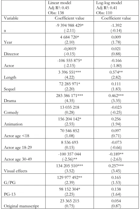
The result of the hypothesis testing can be found in Table 4-3 and was not entirely in line with the predictions. Overall the linear model was shown to be more suitable than the log-log with higher R2_{, higher number of observations included and more significant variables.} Most significant variable coefficients showed the expected sign, except Actor and Actor age 30-49 that was negative.

The final indicator, budget, has previously been found important (see for example Terry et.al (2005)) but as all movies in this sample are blockbusters and thus have a very high budget by definition, the variation within the budget range is not considered important for the purposes of this thesis.

Table 3-3: Hypothesis testing, linear model and log-log model Linear model Adj R2_{: 0.45} Obs: 138 Log-log model Adj R2_{: 0.41} Obs: 110

Variable Coefficient value Coefficient value α -9 394 988 429* (-2.11) (-0.14) -1.392 Year 4 684 720* (2.10) (1.78) 0.009 Director -0,0019 (-0.15) (0.88) 0.021 Actor -106 555 875* (-2.15) (-1.80) -0.166 Length 3 396 551*** (4.22) 0.574** (2.82) Sequel 72 285 971* (2.20) (1.83) 0.111 Drama 283 386 171*** (4.35) 0.462*** (3.35) Comedy 13 035 218 (0.28) (-0.25) -0.023 Animation 156 204 142* (2.55) (1.94) 0.256 Actor age <18 70 546 852 (1.08) (0.71) 0.097 Actor age 18-29 8 536 693 (0.15) (-0.66) -0.073 Actor age 30-49 -100 357 044 (-2.56)** -0.189** (-2.63) Visual effects 134 205 510*** (3.52) 0.257*** (3.45) G/PG 129 977 492** (2.39) (1.53) 0.165 PG-13 98 152 304* (2.25) (1.64) 0.138 Original manuscript 23 365 215 (0.75) (0.87) 0.054

Significant coefficients marked with * (10 percent) ** (5 percent) *** (1 percent). T-values in parenthesis. The chosen indicator for Director is Success, and the coefficient is an indicator of the importance of previous revenue. The chosen indicator for Actor is Talent, and the coefficient is an indicator of the importance of previous Oscar awards. R2_{-values between models cannot be} compared as no intersection variable is used in log-log model.

In Table 3-4 the model of the significant influencers are shown. In this setting the two models’ performance are more alike. The advantage of the log-log model is that it reports changes, not definitive figures, and it will therefore be used for analysis. The interpretation of the changes presented by the log-log model can be found in Table 3-5. All regressions were normally distributed with no heteroscedasticity or multicollinearity.

Table 3-4: Regression result for significant variables, linear and log-log model Linear model Adj R2_{: 0.47} Obs: 162 Log-log model Adj R2_{: 0.45} Obs: 162

Variable Coefficient value Coefficient value α -12 600 000 000*** (-3.84) -3.54479 (-0.65) Year 6 272 314*** (3.84) 0.010074*** (3.72) Actor -135 000 000*** (-3.50) -0.22824*** (-3.56) Length 3 324 676*** (5.29) 0.668181*** (4.81) Sequel 80 293 248*** (2.87) 0.134396*** (2.90) Drama 294 000 000*** (5.24) 0.427747*** (4.60) Visual effects 121 000 000*** (3.76) 0.206581*** (3.87) G/PG 162 000 000*** (3.61) 0.253105*** (3.39) PG-13 96 252 239** (2.58) 0.143228** (2.31) Animation 106 000 000** (2.29) 0.213303*** (2.71) Actor age 30-49 -100 000 000*** (-3.78) -0.15951*** (-3.63)

Significant coefficients marked with * (10 percent) ** (5 percent) *** (1 percent). T-values in parenthesis. The chosen indicator for Director is Success, and the coefficient is an indicator of the importance of previous revenue. The chosen indicator for Actor is Talent, and the coefficient is an indicator of the importance of previous Oscar awards. R2_{-values between models cannot be} compared as no intersection variable is used in log-log model.

Table 3-5: Expected revenue increase. log-log model

Variable Expected increase of revenue, % Length 66.82 Drama 53.38 G/PG 28.80 Animation 23.78 Visual effects 22.95 PG-13 15.40 Sequel 14.38 Year 1.01 Actor age 30-49 -14.74 Actor -20.41

The combined, increased effect of a movie including all positive dummy variables is if the movie is a sequel, a drama, with visual effects nominations, rated G or PG: 14.38 + 53.38 + 22.95 + 28.80 + 15.40 = 111.97% more compared to movies without. According to the results it is possible to more than double movie revenue by including or enhancing certain creative effects! If instead the movie features an Oscar-winning actor aged 30-49 then the

decrease in revenue is -20.41 + (-14.74) = -35.15%. Two unfortunate features of the leading star can according to this model decrease revenue by a third compared to another star.

Due to the uncertainty of the coefficients’ true nature a correlation test was performed. The results are shown in Table 3-6. Most of the significant correlation shown has natural reasons, for example the negative relation between length and movies targeted to children: animations and G/PG-rating.

Table 3-6: Pearson Correlation test

Year Actor Length Sequel Drama Animation Age 30-49 Visual effects G/PG

Year Correlation 1 Sign. Actor Correlation -0.089 1 Sign. 0.259 Length Correlation -0.120 0.040 1 Sign. 0.129 0.614 Sequel Correlation 0.180 -0.109 0.110 1 Sign. 0.022* 0.168 0.162 Drama Correlation -0.252 0.323 0.138 -0.180 1 Sign. 0.001** 0.000** 0.080 0.022* Animation Correlation 0.107 -0.058 -0.491 -0.119 -0.110 1 Sign. 0.176 0.463 0.000** 0.133 0.164 Age 30-49 Correlation -0.021 -0.091 -0.111 0.036 -0.010 -0.002 1 Sign. 0.794 0.251 0.160 0.649 0.898 0.981

Visual effects Correlation -0.183 -0.116 0.399 0.052 -0.051 -0.204 -0.063 1 Sign. 0.020** 0.142 0.000** 0.509 0.518 0.009** 0.427

G/PG Correlation -0.138 -0.080 -0.425 -0.087 -0.186 0.554 -0.056 -0.024 1 Sign. 0.079 0.314 0.000** 0.269 0.018* 0.000** 0.477 0.761

4

Model interpretation

Box office revenue seems to be an assembly of numerous components. The regressions outlined above is taking into account a number of major classifications and possible signal determinants, yet is only explaining 47 percent of the variation in the sample. This has to be considered rather good since there is a large individuality and uniqueness in the observed movies.

The first determining variable, year, is no surprise. Due to the growing global market and inflation adjustments it is reasonable to assume an addition to revenue of 1 percent if the movie is released 1 percent later than planned. This variable should thus be interpreted as rate of inflation + growth rate of the global market.

It appears as though production companies are not exactly meeting the level of quality demanded by the audience. The director variable is an example. Previous revenue of the director did not prove to be a significant influencer. This is quite remarkable: in a marketing setting where movies are presented as the work of the same certain director as this or that movie, without mentioning name, the previous revenue of exactly those movies should be a good determinant of present revenue. This should be especially true in the case of blockbusters where the knowledge rate of previous movies is high, but in this sample this is not so.

Another example is the actor variables. Are actors worth their asking price? No, not according to this sample. Two actor-based variables proved significant: Oscar rewarded actors and the age group 30-49. What is surprising is that both of them have a negative influence. An Oscar rewarded actor decrease the movie revenue with on average 22 percent. This is surprising since Oscar rewarded actors obviously have outperformed a number of other actors earlier in time and should signal quality to the audience. There does not have to be an error in this argument though. As stated previously, the audience’s perception of quality is not dealt with in this paper. Quality is not the same as revenue generation. This would however indicate insignificant results of the Oscar variable, not the negative which is observed. This effect is perhaps due to an inefficient valuation of actors’ performances: castors, directors and producers’ notion of an Oscar is most likely different from the general public, and it is therefore likely that they tend to overvalue it. This would result on a quality level that is perhaps too high for the general public.

The exception is dramas. A drama in this sample have on average 53 percent higher revenue compared to the base group of the most common type, action movies. The category was shown to be positive even after correction of the largest outlier, Titanic. This is although they are correlated with the actor variable. Oscar-receiving actors are thus more often engaged in dramas that on average increase revenue by 50 percent. The explanation could be segmentation: dramas are also negatively correlated with G/PG-rated movies: the audience is an older age group than most other movies on the list.

Animations are also important to the audience. In earlier decades where only one or two animated movies were released yearly they received very much attention. Most of them were Disney productions and although the stories were different the movies were characterized by the same moral values and themes (the sample includes movies like The Lion King, Aladdin, Pocahontas and The Hunchback of Notre Dame). It is difficult to imagine a

Disney movie from this era that would chock or surprise the audience; the validity of the audiences’ experience set is very high concerning these movies. The highest ranked movies in the sample is however newer movies. Long gone are the days when animated movies were rare and this segment of the market is now almost as easy to supply as any other. Yet animated movies are similar to movies with visual effects nominations: they are extraordinary. The technological setting of animations is still evolving and many movies on the list have been very technologically advanced on their release dates (Toy Story, Finding Nemo and Ice Age).

Previous consumption experiences of similar kind seem to be a good way of increasing willingness to pay. Sequels, which are trying to increase revenue through strong associations to previous similar movies is significant as a determinant. It appears as though sequels as a concept, not just the recent film series where the end is not exposed until the last movie, is an efficient method for increasing willingness to pay. Although sequels are sometimes perceived as ‘shortcuts’ by the audience and not really a ‘real’ movie, their engagement to the first movie is apparently influencing their expectations about the following.

The connection between an original manuscript and revenue is on the other hand not significant, although the presence of a book or comic is somewhat similar to a sequel: the setting of characters and the story is familiar to the audience. The insignificance could be due to differences in imagery, structure and narration: although a book and a movie present the same core story, the rules of communication are not the same in books and movies. A movie is simply a completely different way of telling a story (Lothe, 2000). The signal effect for a satisfied reader is therefore limited if he/she does not believe that the movie will be a similar experience as to reading the book.

4.1 The unique variables

Whether the hypothesis that the audience is trying to maximize value by seeing movies that are exploiting the technological setting in cinemas is confirmed or not is a complex question. The kind of movies that normally are associated with special effects, like action movies, did not prove to be important. Action movies are however still the most common category in the sample although they are not produced in majority. The other indicator of technological advancement, the dummy for visual effects Oscar nomination, turned out to be important. Whether the movie is visually spectacular or not, is better determined with whether they are up for an Oscar than whether they belong to a certain category. The top movie on the list, Titanic, is perhaps the best example of this: it is neither an action nor an adventure movie, yet its technological spectacularity when it premiered was immense. The other unique variable, length, did also prove to be significant. The sometimes perceived opinion that movies has grown longer lately was proven false in the correlation test, it even showed negative results. The effect on revenue from an increase in length is therefore direct. This may seem perplexing at first sight, is it really so that audiences are so economically aware that they assess a movie by the minutes? Perhaps, or the effect is a combination of this and a signal effect. Length is a confidence indicator: this movie is good enough to run two hours without boring the audience and there is so much effort put into it that it impossibly can be shortened.

4.2 Beyond the model

This section tries to outline possible explanations for the remaining 53 percent variation that is not accounted for in the econometric model. The expected results versus the actual are shown below in Figure 4-1. There is a difference in pattern on the two sides of the 45 degree line: the over-performers are scattered on a large area whereas the under-performers are closely connected. The pattern follows the one outlined in Figure 4-1.

Figure 4-1: Expected versus observed revenue

is a privilege but Table 4-1 and 4-2 are presenting the top ten over-performers and under-performers according to the model. Six out of ten movies among the top performers are sequels along with four of the worst. Making sequels have proven to be an important determinant but is risky, having a potential audience with a very specific set of expectations

also limits creative possibilities in order not to “disappoint” consumers.

The ten over-performers is at first sight a rather mixed group: one animation, one trilogy and various sequels. One distinctive feature emerges however: seven out of ten movies’

secondary category is Adventure (exceptions are Titanic, Spider-Man and Spider-Man 2). Is it perhaps so that audiences do care about thrilling camera movements, sound effects and excitement after all, but not in the anticipated action setting but instead in adventures? Adventure is in a sense a broader term than action movies; it is commonly used as a secondary explanatory category. It therefore reveals, in similarity with visual effects, more about the experience itself than the story. This broader term is also creating a larger target group: a larger possible audience is pr nture movie than an action movie.

Table 4-1: Top v

Rank Expe Obs Di

obably attracted to an adve ten o er-performers

Title cted erved fference

Titanic 1 1 082 050 441 1 835 300 000 753 249 559

Jurassic Park 9 319 207 893 919 700 000 600 492 107

Star Wars: Episode I - The Phantom Menace 7 522 830 842 922 379 000 399 548 158 Pirates of the Caribbean: Dead Man's Chest 3 678 508 771 1 060 332 628 381 823 857

Spider-Man 3 11 527 209 649 885 430 303 358 220 654

Shrek 2 12 527 205 372 880 871 036 353 665 664

Spider-Man 18 455 710 663 806 700 000 350 989 337

Harry Potter and the Sorcerer's Stone 4 618 251 066 968 657 891 350 406 825

Spider-Man 22 433 496 595 783 577 893 350 081 298

Pirates of the Caribbean: At World's End 5 623 625 253 958 404 152 334 778 899

In the under-performers there is no single explanatory trend. Among the four sequels none manage to collect more revenue than its predecessor, indicating that they have in some way not satisfied the audience’s expectations based on the first film. Two movies (American Beauty and Rain Man) are in budgetary sense immense successes: they have both very small e perhaps not fitting very well in this model f blockbusters: the very definition of a blockbuster imply a large budget.

Table 4-2: Top d s

R E Obs D

budgets compared to the rest. They are therefor o

ten un er-performer

Title ank xpected erved ifference

Over the Hedge 146 647 209 992 329 619 340 -317 590 652 Ocean's Thirteen 162 591 690 157 311 144 465 -280 545 692 Basic Instinct 121 631 683 340 352 700 000 -278 983 340 Back to the Future Part II 144 597 990 802 332 000 000 -265 990 802 Live Free or Die Hard 103 637 994 317 377 520 804 -260 473 513 The Devil Wears Prada 153 561 903 807 324 432 962 -237 470 845 Pocahontas 132 574 889 862 347 100 000 -227 789 862 The World Is Not Enough 123 561 459 701 352 000 000 -209 459 701

Rain Man 89 605 542 140 412 800 000 -192 742 140

5

Conclusions

This paper’s aim was to outline a general model of the indicators of box office revenue for the top performing movies in history. The experience industry is different from most other in that the consumer good consist to a large extent of an emotion arousal. It thus lacks many of the features of normal consumption goods: it cannot be reversed or returned and it cannot be stored. The consumption experience is thus entirely based on previous experiences of similar kind.

Demand for experiences has two important influencers: income and leisure time. An increase in any of the two will increase demand for movie tickets. Since the effect of an income increase both can lead to leisure time increases and decreases the effect of higher wages on demand is complex to predict. Production of experiences is based on a combination of an available set of attributes that are combined into goods in a monopolistic competition setting. These form a level of quality that in optimum matches the audiences’ willingness to pay for quality. It is assumed that quality is a function of educated labour. This labour is able to earn very high wages although their talent is only marginally smaller than others.

The different quality attributes were measured using hedonic price theory. This allows to price every unique attribute of movies individually based on what the willingness to pay was in previous movies. The results showed that attributes such as category, actor, sequels, MPAA rating, length and visual effects are important to the audience. The insignificance of some variables, such as director and the negativity of the actor-variable is indicating that the movie industry is not entirely meeting the audience’s quality demands. The two most valuable categories were shown to be dramas and animations, but the pattern of over-performers is indicating that a secondary category, adventure, could also have significant importance. Some consumer segments are possible to outline: the significance of animations along with MPAA’s lowest ratings is for example pointing towards the young. All these are to various degrees based on previous consumption experiences and the strongest variable indicating riskless expectancies, sequels, is shown to be positive.

The outstanding trend among the top performers was suspected to be the secondary category adventure. This category has tight connections with visual effects, one of the most robust variables of the sample. This is thus one interesting issues for further research, what influence does secondary category have? Are they perhaps telling more to the story than the first? Another interesting feature is to look at what film theorists call “high-concept”-films. These are films that easily appeal to large audiences and have an idea that is easily communicated to the audience. Most block-busters are high-concept films, and it could therefore be interesting to evaluate this sample from this perspective. Variables that are important in this setting but not included in this paper are for example soundtrack and consumption of licensed merchandise.

Another topic that should be further investigated is the importance of talent and fame. The model in this paper presented two types of measurements for director’s importance and three for actors, but the results did not meet expectations. Is there any other way to measure fame that is more productive? Is perhaps the combination of actors more important than the actors as individuals?

References

Albert, S. (1998). Movie stars and the distribution of financially successful films in the motion-picture industry. Journal of Cultural Economics. Vol 22, No 4.

Andersson, Å.E., Andersson, D.E. (2006). The economics of experiences, the arts and entertainment. Cheltenham: Edward Elgar

Babin, B.J., Darden, W.R., Griffin, M. (1994). Work and/or Fun: Measuring Hedonic and Utilitarian Shopping Value. The Journal of Consumer Research. Vol 20, No 4.

Bagella, M., Becchetti, L. (1999). The Determinants of Motion Picture Box Office Performance: Evidence form Movies Produced in Italy. Journal of Cultural Economics. Vol 23, No 4.

Banker, A. (2001). Bollywood. Harpenden: Pocket Essentials.

Basuroy, S., Chatterjee, S., Ravid, S.A. (2003). How Critical are Critical Reviews? The Box Office Effects of Film Critics, Star Power and Budgets. Journal of Marketing. Vol 67, No 4.

Bordwell, D. (2000). Planet Hong Kong: Popular Cinema and the Art of Entertainment. Cambridge, MA: Harvard University Press.

Brems, H. (1968). Quantitative Economic Theory: A synthetic Approach. New York: John Wiley & Sons Inc

Caves, R. E. (2000). Creative Industries: Contracts Between Art and Commerce. Cambridge & London: Harvard University Press.

Chadhuri, A., Holbrook, M.B. (2001). The Chain of Effects from Brand Trust and Brand Affect to Brand Performance: The Role of Brand Loyalty. Journal of Marketing. Vol 65 No 2.

Chung, K. H., Cox, R. A. (1994). A Stochastic Model of Superstardom: An Application of the Yule Distribution. The Review of Economics and Statistics. Vol 76, No 4.

Chung, K. H., Cox, R. A. (1998). Consumer behavior and superstardom. Journal of Socio-Economics. Vol 27, No 2.

Cropper, M.L., Deck, L.B., McConnel, K.E. (1988). On the Choice of Functional Form for Hedonic Price Functions. The Review of Economics and Statistics. Vol 70, No 4. Davis, P. (2001). Spatial Competition in Retail Markets: Movie Theaters. Journal of

Economics. Vol 37, No 4.

De Vany, A.S. (2004). Hollywood economics : how extreme uncertainty shapes the film industry. New York : Routledge.

Eliashberg, J., Sawhney, M.S. (1994). Modeling Goes to Hollywood: Predicting Individual Differences in Movie Enjoyment. Management Science. Vol 40, No 9.

Frey, B.S. (2001). What Is the Economic Approach to Aesthetics? In N.S. Baer & F. Snickars (eds), Rational Decision-making in the Preservation of Cultural Property. Berlin: Dahlem University Press.

Ginsburgh, V., Weyers, S. (1999). On the Perceived Quality of Movies. Journal of Cultural Economics. Vol 23, No 4.