Exploration and Exploitation in Reinforcement Learning

IN

DEGREE PROJECT

TECHNOLOGY,

FIRST CYCLE, 15 CREDITS

,

STOCKHOLM SWEDEN 2018

Exploration and Exploitation

in Reinforcement Learning

FELIX ADELSBO

INOM

EXAMENSARBETE

TEKNIK,

GRUNDNIVÅ, 15 HP

,

STOCKHOLM SVERIGE 2018

Utforskning och utnyttjande

inom förstärkande inlärning

Abstract

In reinforcement learning there exists a dilemma of exploration versus exploitation. This has led to the development of methods that have di↵er-ent approaches to this. Using di↵erdi↵er-ent types of methods, and modifying them in di↵erent ways can lead to di↵erent results. Knowledge of how di↵erent methods work can give knowledge of what should be used in a specific case.

Two ways that methods can be modified are change in adjustable pa-rameters and change in the number of steps of random actions at the beginning. How much these two modifications e↵ect the results in a spe-cific environment may di↵er a lot, and can be a very critical thing to consider for certain results.

The goal of this study is to answer the question of how the performance of the di↵erent methods such as random, greedy, ✏-greedy, ✏-decreasing and Softmax is a↵ected by di↵erent values of their adjustable parameters, and by the number of steps of random actions at the beginning. The simulations and a comparative analysis are conducted for the case of an inverted pendulum with a vertical pole placed on a moving cart.

Sammanfattning

Inom f¨orst¨arkande inl¨arning existerar ett dilemma inom utforskning kontra utnyttjande. Detta har lett till utvecklandet av metoder som har olika tillv¨agag˚angss¨att f¨or detta. Att anv¨anda olika typer av metoder, och modifiera dem p˚a olika s¨att kan leda till olika resultat. Kunskap om hur olika metoder fungerar kan ge kunskap om vad som ska anv¨andas i ett specifikt fall.

Tv˚a s¨att som metoder kan modifieras ¨ar ¨andring i justerbara parametrar och ¨andring i antalet slumpm¨assiga steg i b¨orjan. Hur mycket dessa tv˚a modifieringar p˚averkar resultatet i en specifik milj¨o kan skilja sig mycket ˚at, och kan vara en v¨aldigt kritisk sak att bet¨anka f¨or ett visst resultat.

M˚alet med denna studie ¨ar att besvara fr˚agan om hur prestandan p˚a de olika metoderna random, greedy, ✏-greedy, ✏-decreasing och Softmax p˚averkas av olika v¨arden p˚a deras justerbara parametrar, och av antalet slumpm¨assiga steg i b¨orjan. Simuleringarna och en j¨amf¨orande analys utf¨ors f¨or fallet med en inverterad pendel med en vertikal stolpe placerad p˚a en r¨orlig vagn.

Contents

1 Introduction 1

1.1 Exploration and exploitation . . . 1

1.2 Purpose . . . 1 1.3 Hypothesis . . . 2 1.3.1 Random method . . . 2 1.3.2 Greedy method . . . 2 1.3.3 ✏-greedy method . . . 2 1.3.4 ✏-decreasing method . . . 2 1.3.5 Softmax method . . . 2 2 Background 3 2.1 Related work . . . 3 2.2 Reinforcement learning . . . 4 2.3 Performance . . . 5 2.4 Q-network . . . 5 2.4.1 Q-learning . . . 5 2.4.2 Deep Q-learning . . . 5 2.5 Experience methods . . . 5 2.5.1 Random method . . . 6 2.5.2 Greedy method . . . 6 2.5.3 ✏-greedy method . . . 6 2.5.4 ✏-decreasing method . . . 6 2.5.5 Softmax method . . . 6 2.6 Description of environment . . . 6 2.6.1 Observation . . . 7 2.6.2 Actions . . . 7 2.6.3 Reward . . . 7 2.6.4 Episode termination . . . 8 2.7 Test of performance . . . 8 3 Results 9 3.1 Random method . . . 9 3.2 Greedy method . . . 11

3.2.1 Greedy method with 50000 steps of random actions . . . 11

3.3 ✏-greedy method . . . 14

3.3.1 ✏-greedy with 50000 steps of random actions for ✏=0.9 . . 15

3.3.2 ✏-greedy with 50000 steps of random actions for ✏=0.5 . . 17

3.3.3 ✏-greedy method with 50000 steps of random actions for ✏=0.1 . . . 20

3.4 ✏-decreasing method . . . 23

3.4.1 ✏-decreasing method with 50000 steps of random actions . 23 3.4.2 ✏-decreasing method with 100000 steps of random actions 26 3.5 Softmax method . . . 29

3.5.2 Softmax method with 100000 steps of random actions . . 32

3.6 Comparing the results . . . 36

3.6.1 Kruskal–Wallis test . . . 36 3.6.2 Dunn’s test . . . 36 4 Discussion 39 4.1 Analysis of methods . . . 39 4.1.1 Random method . . . 39 4.1.2 Greedy method . . . 39 4.1.3 ✏-Greedy method . . . 39 4.1.4 ✏-decreasing method . . . 39 4.1.5 Softmax method . . . 39 4.2 Critical evaluation . . . 40 4.3 Implications . . . 40 4.4 Future research . . . 41 5 Conclusions 41 References 42 A Appendix 43 A.1 Source code for the cart-pole environment . . . 43

1

Introduction

1.1

Exploration and exploitation

In order for an agent to perform optimally in an environment, it needs to be exposed to as many of the states in the environment as possible. In reinforce-ment learning you only have access to the environreinforce-ment through the actions. This creates a problem where the agent needs the right experiences to learn a good policy, but it also needs a good policy to obtain those experiences. This dilemma has led to the development of techniques for balancing exploration and exploitation.

There are di↵erent approaches to select actions, which handles exploration and exploitation in di↵erent ways. By using the di↵erent types of methods, and modifying them in di↵erent ways, you can get di↵erent results. Knowledge of how di↵erent methods work can give knowledge of what should be used in a specific case.

Two ways that methods can be modified are change in adjustable parameters and change in number of steps of random actions at the beginning. How much these two modifications e↵ects the results in a specific environment may di↵er a lot, and can be a very critical thing to consider for certain results.

1.2

Purpose

The goal of this study is to answer the question of how the results of the dif-ferent methods random, greedy, ✏-greedy, ✏-decreasing and softmax is a↵ected by di↵erent values of their adjustable parameters, and by the number of steps of random actions at the beginning, for the environment described in 2.6. To answer it, the following will be investigated:

• Which of the methods: random, greedy, ✏-greedy, ✏-decreasing and soft-max gives the highest reward?

• How is the reward spread out over the iteration steps for the methods: random, greedy, ✏-greedy, ✏-decreasing and softmax?

• How does a change in value of ✏ e↵ect the amount and spread in reward for the ✏-greedy method?

• How does a change in the amounts of steps of random actions at the earlier stage e↵ect the amount and spread in reward for the methods: ✏-decreasing and softmax?

These are things that involve di↵erent types of changes in exploration and exploitation of the methods. By investigating this, an attempt is made to give better knowledge of what type of approach that is suitable in terms of value of adjustable parameters and number of steps of random actions at the beginning.

1.3

Hypothesis

1.3.1 Random method

The fact that this method only is optimal in an environment where a random approach is optimal, it is not expected be the method that gives the highest reward.

The total regret is linear with a method that always explores, which also indicates that the method is not the one that give the highest reward.

1.3.2 Greedy method

It is not expected to be a good approach to always choose the option which is believed to give the highest reward. The system seems be too complex for this method to reach an optimal solution. The agent might need more exploration. The total regret is linear with a method that always exploits, which indicates that the method is not the one that will give the highest reward. However, it is expected to give higher reward than the random method, because of the steps of random actions at the beginning.

1.3.3 ✏-greedy method

This is expected to give better result than the greedy method, because more exploration is possible. This gives an opportunity to choose other actions than what is considered optimal, which may give higher reward. However, the method only takes into account if an action is optimal or not, which can stop it from doing experiences in an optimal way. The system might so complex that expe-rience needs to be seen in a more careful way, where di↵erent approaches are seen as more promising than others.

1.3.4 ✏-decreasing method

This is expected to give higher result than the ✏-greedy method, because explo-ration is more encourage in the beginning. This might e↵ect its way of deciding what action that is optimal. Still, it faces the same problem as the ✏-greedy method, where it only takes into account if an action is optimal or not, which can stop it from doing experiences in an optimal way.

1.3.5 Softmax method

This method is expected to give the highest reward, because it not only sees if an action is optimal or not, but also takes into account how promising the other actions are. If the probabilities are weighted in a reliable way, this might lead to a form of exploration that can give higher rewards.

2

Background

2.1

Related work

Much research has been done in reinforcement learning, where di↵erent issues have been addressed. Examples of issues can be to achieve efficient exploration in complex domains [1], to handle environments containing a much wider variety of possible training signals [2], lack of generalization capability to new target goals [3], data inefficiency where the model requires several episodes of trial and error to converge [3] or making an intelligent agent able to act in multiple environments and transfer previous knowledge to new situations [4].

These issues have resulted in many di↵erent types of research. One exploration method used has been based on assigning exploration bonuses from a concur-rently learned model of the system dynamics. By parameterizing the learned model with a neural network, an efficient approach to exploration bonuses was developed, that could be applied to tasks with complex, high dimensional state spaces [1].

An agent has been introduced that maximizes many other pseudo-reward func-tions simultaneously [2].

An actor-critic model has been proposed, whose policy is a function of the goal as well as the current state, which allows to better generalize [3]. An AI2-THOR framework has been proposed, which provides an environment with 3D scenes and physics engine. The framework enables agents to make actions and interact with objects, and a big number of training samples can be collected efficiently [3].

A method of multitask and transfer learning has been defined, that enables an autonomous agent to learn how to behave in multiple tasks simultaneously, and then generalize its knowledge to new domains [4].

Convolutional neural network trained with a variant of Q-learning has been used to learn control policies directly from high-dimensional sensory input, whose in-put is raw pixels and whose outin-put is a value function estimating future rewards. The method was applied to Atari 2600 games [5].

Deep Q-Learning, with an algorithm based on the deterministic policy gradient that can operate over continuous action spaces has been used to solve many simulated physics tasks [6].

A recurrent network has been used to generate the model descriptions of neural network and train this network with reinforcement learning to maximize the expected accuracy of the generated architectures on a validation set [7]. Deep reinforcement learning has been applied to model future reward in chat-bot dialogue [8].

Cesar Bianchi and Fisher proved poly-logarithmic bounds for variants of the algorithm in which ✏ decreases with time [9]. Vermorel and Mohri got that ✏ decreasing method did not significantly improve the performance compared to the ✏-greedy method [10]. In this test, the ✏-greedy and ✏-decreasing will therefore not primarily be compared with each other, but instead the ✏-greedy method will be compared with di↵erent values of ✏ and ✏-decreasing method

with di↵erent amounts of steps of random actions at the beginning.

Vermorel and Mohri also got similar result for the softmax method for dif-ferent values of ⌧ [10]. In this test, the sofmax method will therefore only be tested with change in the number of random steps at the beginning, and not with di↵erent constant values of ⌧ .

2.2

Reinforcement learning

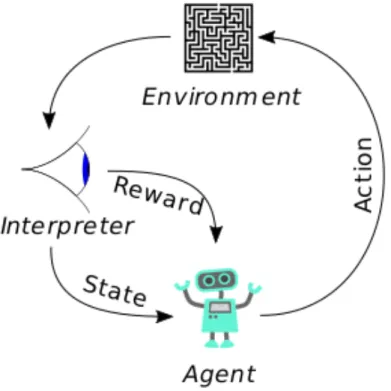
Reinforcement learning is an area of machine learning concerned with how agents should take actions in an environment so as to maximize a cumulative reward. In basic terms, a model of reinforcement learning contains an agent who takes actions in an environment. These actions gives a reward and a representation of the state, which are fed back to the agent.

Figure 1: Model of reinforcement learning.

Figure 1 shows a basic visualization of a model in reinforcement learning. If the model contains a set of states, S, and a set of actions, A, of the agent, then the probability of transition from s to state s0 _{under action a is Pa(s, s}0_{) =} P r(st+1 = s0 _{| s} = s, at= a). The transition from s to s’ with action a result

The interaction is done in discrete time steps. At time t, the agent chooses an action at, which makes the environment to move to a new state st+1and the reward rt+1is received from the transition (st, at, st+1).

Through this process, the goal is to collect as much reward as possible [11].

2.3

Performance

The performance is measured by the size of the total reward, rN, for each episode, where N is the total amount of iteration steps in an episode. When an episode begins, the total reward is set to zero, r0 = 0, and a reward of 1 point is added to it for every iteration step taken, rt+1= rt+ 1, including the termination step. After the termination the total reward is stored, then the process is repeated with a new episode and a new total reward set to zero.

2.4

Q-network

2.4.1 Q-learning

Q-learning contains a table of values for every state and action possible. The Q-table changes though the Bellman equation,

Q(s, a) = r + max(Q(s0, a0)).

(1) where Q(s, a) is the Q-value for state s and action a, is a discount factor and max(Q(s0_{, a}0_{)) is the maximum future reward expected for the next state. The} equation states that the long-term expected reward is equal to the immediate reward together with the reward expected from the best future action in the next state [12].

2.4.2 Deep Q-learning

Deep Q-learning (DGN) is a variation of Q-learning with 3 main contributions: 1. Multi-layer convolutional net architecture.

2. Implementing batches of data, which allow the network to use stored mem-ories to train itself.

3. Use of older network parameters to estimate the Q-values of the next state [12].

This is used to test the di↵erent methods.

2.5

Experience methods

The experience methods that will be use are random, greedy, ✏-greedy, ✏-decreasing and softmax.

2.5.1 Random method

A random action is always taken and the environment is being explored. 2.5.2 Greedy method

A naive approach, where the action which the agent expects to give the greatest reward is always chosen.

2.5.3 ✏-greedy method

With probability 1-✏ an action with the greatest expected reward is chosen, and with probability ✏ a random action is chosen.

The value of ✏ can be adjusted [13]. 2.5.4 ✏-decreasing method

This is like the ✏-greedy method, but with a value of ✏ that decreases in the progress. This results in more exploration at the earlier stage, and more ex-ploitation at a later stage.

2.5.5 Softmax method

An action is chosen with weighted probabilities. The function used is

Pt(s, a) = eQt(a)⌧ Pn i=1e Qt(i) ⌧ , (2) where ⌧ is a temperature parameter, which controls the spread of the soft-max distribution.

For high values of ⌧ , the actions have probabilities closer to each other, and for low values of ⌧ , the probability of the action with highest expected reward is bigger [13].

2.6

Description of environment

The environment that will be used for the study is from OpenAI Gym [14]. It consists of a pole, which is attached by an un-actuated joint to a cart, which moves along a frictionless track. The pendulum starts upright, and the goal is to prevent it from falling over by increasing and reducing the carts velocity. A visualization of the environment is shown in figure 2 [15].

Figure 2: The Cart-Pole Environment 2.6.1 Observation

Number Observation Minimum Maximum 0 Cart Position -2.4 2.4 1 Cart Velocity -Inf Inf 2 Pole Angle _{⇠-41.8 ⇠ 41.8} 3 Pole Velocity At Tip -Inf Inf

Table 1: Number, observation, minimum and maximum for the environment.

2.6.2 Actions

Number Action

0 Push cart to the left 1 Push cart to the right

Table 2: Number and action for the environment.

2.6.3 Reward

2.6.4 Episode termination 1. Pole Angle is more than±12 .

2. Cart Position is more than _{±2.4 (center of the cart reaches the edge of} the display).

3. Episode length is greater than 1000.

This means that an episode ends when the pole leans more than 12 on either side. That the cart position is more than _{±2.4 means that the cart} reaches the edge of the display on the left or the right side. That the episode length is greater than 1000 means that the episode ends when it has reaches 1000 iteration steps.

2.7

Test of performance

For each method, the test will be performed in 20000 episodes. One plot with reward and another plot with average reward per 1000 episodes will be shown and compared.

For the average reward per 1000 episodes the standard deviation, s, will be calculated. This is done by using

s = qPN

i=1(ri r)2

N 1 ,

(3) where_{r1, r2, ..., rN_{} are the values of the rewards, r is the average value of} these rewards, and N is the number of rewards. s will be shown as error bars on the plot for the average reward per 1000 episodes.

The ✏-greedy method will be tested with 50000 steps of random actions at the beginning for ✏=0.9, ✏=0.5 and ✏=0.1. The ✏-decreasing method and soft-max method will be tested for 50000 and 100000 steps of random actions at the beginning.

3

Results

3.1

Random method

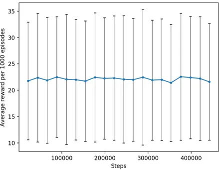
Figure 4: Average reward per 1000 episodes of the random method. Error bars with the value of s.

In figure 3, the reward is spread around 0 and 150, with most results around 0 and 80. Neither lower or higher rewards seems to be more common along with the iteration steps. The improvement is considered low.

In figure 4, the average reward is spread around 21.3 to 23.0. The average reward is stable and does not change remarkably along the iteration steps. That the improvement is low is not surprising, because the method is only based on random actions, where the exploration is not used in any way to im-prove the result. There is some di↵erence in values, which is possible in this random process, but the randomness also causes the probability for a certain value to never change. This is why the spread of values looks similar over all iteration steps.

Number of steps Average reward s 21776 21.76 11.16 44166 22.39 12.23 66030 21.86 11.93 88536 22.51 11.47 110593 22.06 12.36 132582 21.99 11.43 154302 21.72 11.43 176733 22.43 12.27 198976 22.24 11.52 221288 22.31 11.80 243354 22.07 12.10 265349 22.00 11.66 287806 22.46 12.85 309725 21.92 11.40 331726 22.00 11.55 353130 21.40 11.11 375692 22.56 12.06 398095 22.40 11.62 420319 22.22 11.75 441908 21.59 11.07

Table 3: Number of steps, average reward and value of s for the random method.

3.2

Greedy method

The test was made with 50000 steps of random actions.

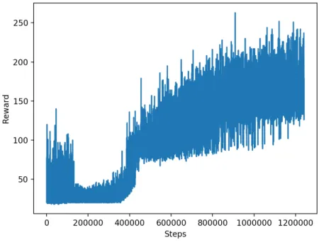
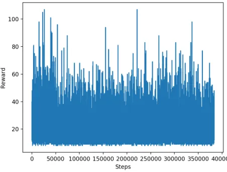
Figure 5: Reward of the greedy method and 50000 steps of random actions at the beginning.

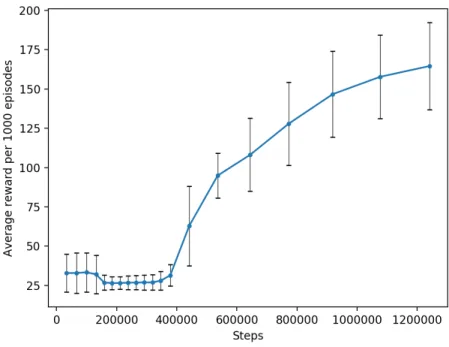
Figure 6: Average reward per 1000 episodes of the greedy method with 50000 steps of random actions at the beginning. Error bars with the value of s.

In figure 5, the reward is spread around 0 and 300, with a remarkable di↵er-ence in common appearance of higher reward. Lower rewards seem to get more uncommon and higher rewards more common as the iteration steps increases. Along the steps of random actions it makes improvements, and when they stop there is a relatively small decrease in rewards until around 300000 steps, after that it starts to increase a lot.

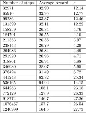
In figure 6, the average reward is spread around 0 and 170. The amount of average reward increases along the steps of random actions, then there is a rel-atively small decrease until around 300000 steps, after that it starts to increase a lot.

That it makes such a big improvement after 400000 iteration steps might be because it then got to a point where choosing the action that gave the highest expected reward was the right way to go, because the expectation was close to the optimal.

Number of steps Average reward s 32971 32.90 12.14 65916 32.95 12.77 99286 33.37 12.46 131399 32.11 12.22 158239 26.84 4.76 184791 26.55 4.10 211353 26.56 3.97 238143 26.79 4.29 264986 26.84 4.49 291920 26.93 4.71 318861 26.94 4.88 346930 28.07 5.95 378424 31.49 6.72 441248 62.82 25.34 536165 94.92 14.15 644283 108.1 23.18 772129 127.9 26.33 918774 146.7 27.26 1076457 157.7 26.54 1240999 164.5 27.73

Table 4: Number of steps, average reward and value of s for the greedy method.

3.3.1 ✏-greedy with 50000 steps of random actions for ✏=0.9

Figure 7: Reward for episodes of the ✏-greedy method with ✏=0.9 and 50000 steps of random actions at the beginning.

Figure 8: Average reward per 1000 episodes of the ✏-greedy method with ✏=0.9 and 50000 steps of random actions at the beginning. Error bars with the value of s.

In figure 7, the reward is spread around 0 and 120. Lower rewards seem to be a bit more common along with the iteration steps. The improvement is considered low.

In figure 8, the average reward is spread around 17.0 and 22.5. There is a remarkable decrease in average reward along the iteration steps.

Number of steps Average reward s 22080 22.07 11.63 44488 22.41 12.44 64091 19.60 9.89 82629 18.54 8.61 101173 18.54 8.80 119912 18.74 8.42 138276 18.36 8.42 157196 18.92 9.20 176073 18.88 9.05 194754 18.68 8.66 213529 18.78 8.82 232187 18.66 9.47 250799 18.61 9.01 269653 18.85 9.01 288650 19.00 9.21 308003 19.35 9.53 327686 19.68 9.78 346832 19.15 9.42 365212 18.38 8.44 383555 18.34 8.29

Table 5: Number of steps, average reward and value of s for the ✏-greedy method with ✏=0.9.

Figure 9: Reward for episodes of the ✏-greedy method with ✏=0.5 and 50000 steps of random actions at the beginning.

Figure 10: Average reward per 1000 episodes of the ✏-greedy method with ✏=0.5 and 50000 steps of random actions at the beginning. Error bars with the value of s.

In figure 9, the reward is spread around 0 and 120, with very remarkable di↵erence in common appearance of lower reward after the 50000 steps of ran-dom actions.

In figure 10, the average reward is spread around 10.0 and 24.0. There is a remarkable decrease in average reward after the 50000 steps of random actions.

Number of steps Average reward s 22877 22.86 12.10 44053 21.18 10.72 59103 15.05 7.45 71381 12.28 3.31 83594 12.21 3.03 95801 12.21 3.39 107979 12.18 3.26 120158 12.18 3.15 132302 12.14 2.97 144458 12.16 3.15 156339 11.88 2.79 168468 12.13 3.25 180715 12.25 3.20 192685 11.97 2.75 204705 12.02 2.78 216884 12.18 3.22 229103 12.22 3.31 241246 12.14 3.34 253400 12.15 2.90 265650 12.25 3.22

Table 6: Number of steps, average reward and value of s for the ✏-greedy method with ✏=0.5.

Figure 11: Reward for episodes of the ✏-greedy method with ✏=0.1 and 50000 steps of random actions at the beginning.

Figure 12: Average reward per 1000 episodes of the ✏-greedy method with ✏=0.1 and 50000 steps of random actions at the beginning. Error bars with the value of s.

In figure 11, the reward is spread around 0 and 100, with very remarkable di↵erence in common appearance of lower reward after the 50000 steps of ran-dom actions.

In figure 12, the average reward is spread around 8 and 24.0. There is a re-markable decrease in average reward after the 50000 steps of random actions. That this method makes a big decrease in rewards after the ending of the steps of random actions is probably because there has not been enough of exploration until it starts to take actions that will result in the highest expected reward. The exploration might not result in expectations that is actually close to opti-mal, and if it is very far from optimal it can lead to a big decrease in rewards after the ending of the steps of random actions, which is the case in this test.

Number of steps Average reward s 22500 22.49 11.94 44550 22.05 11.35 57574 13.02 8.23 67459 9.885 1.05 77287 9.828 1.11 87034 9.747 1.09 96822 9.788 1.15 106520 9.698 1.07 116269 9.749 1.08 126018 9.749 1.16 135721 9.703 1.06 145481 9.760 1.09 155260 9.779 1.04 165017 9.757 1.09 174798 9.781 1.07 184599 9.801 1.08 194293 9.694 1.07 204012 9.719 1.04 213772 9.760 1.06 223522 9.750 1.11

Table 7: Number of steps, average reward and value of s for the ✏-greedy method with ✏=0.1.

3.4

✏-decreasing method

The test was made with 50000 and 100000 steps of random actions. 3.4.1 ✏-decreasing method with 50000 steps of random actions

Figure 13: Reward for episodes of the ✏-decreasing method with 50000 steps of random actions at the beginning.

Figure 14: Average reward per 1000 episodes of the ✏-decreasing method with 50000 steps of random actions at the beginning. Error bars with the value of s.

In figure 13, the reward is spread around 0 and 700, with remarkable increase in common appearance of higher rewards along the iteration steps.

In figure 14, the average reward is spread around 20.0 and 160.0. There is a remarkable increase in average reward along the iteration steps.

Number of steps Average reward s ✏ 21994 21.98 11.74 1.0000 44919 22.93 12.97 1.0000 67633 22.71 12.36 0.9647 90121 22.49 11.33 0.9198 112614 22.49 11.23 0.8748 136638 24.02 11.89 0.8267 163733 27.10 13.17 0.7725 193842 30.11 15.70 0.7123 231476 37.63 20.18 0.6371 273847 42.37 20.24 0.5523 321956 48.11 21.04 0.4561 378609 56.65 23.50 0.3428 448875 70.27 28.36 0.2023 536345 87.47 34.76 0.1000 636436 100.10 37.90 0.1000 750962 114.53 45.55 0.1000 876173 125.21 50.02 0.1000 1006328 130.16 56.37 0.1000 1143710 137.38 58.01 0.1000 1286581 142.87 63.02 0.1000

Table 8: Number of steps, average reward, value of s and value of ✏ for the ✏-decreasing method with 50000 steps of random actions at the beginning.

Figure 15: Reward for episodes of the decaying ✏-decreasing method with 100000 steps of random actions at the beginning.

Figure 16: Average reward per 1000 episodes of the ✏-decreasing method with 100000 steps of random actions at the beginning. Error bars with the value of s.

In figure 15, the reward is spread around 0 and 600, with remarkable increase in common appearance of higher rewards along the iteration steps.

In figure 16, the average reward is spread around 20.0 and 160.0. There is a remarkable increase in average reward after the 100000 steps of random ac-tions.

The increase is remarkable in relation to the big decrease of the ✏-greedy method. Because of the slower shift from higher to lower value of ✏, there is not the same problem with having wrong expectations of high rewards, but there is instead a higher probability of exploration after the ending of the steps of random actions.

Number of steps Average reward s ✏ 22096 22.08 12.08 1.0000 44456 22.36 12.01 1.0000 66983 22.53 12.46 1.0000 89096 22.11 11.70 1.0000 111334 22.24 11.92 0.9773 135054 23.72 13.17 0.9299 161247 26.19 14.80 0.8775 191670 30.42 16.66 0.8167 224850 33.18 19.11 0.7503 261194 36.34 19.37 0.6776 303731 42.54 21.30 0.5925 355759 52.03 25.47 0.4885 416463 60.70 28.79 0.3671 487543 71.08 30.65 0.2249 575761 88.22 37.35 0.1000 679141 103.4 40.48 0.1000 797138 118.0 50.80 0.1000 925258 128.1 55.23 0.1000 1068364 143.1 66.18 0.1000 1218621 150.3 67.83 0.1000

Table 9: Number of steps, average reward, value of s and value of ✏ for the ✏-decreasing method with 100000 steps of random actions at the beginning.

3.5

Softmax method

The test was made with 50000 and 100000 steps of random actions. 3.5.1 Softmax method with 50000 steps of random actions

Figure 17: Reward for episodes of the softmax method with 50000 steps of random actions at the beginning.

Figure 18: Average reward per 50 episodes of the softmax method with 50000 steps of random actions at the beginning. Error bars with the value of s.

In figure 17, the reward is spread around 0 and 160, with a very remarkable di↵erence in common appearance of lower reward after the 50000 steps of ran-dom actions.

In figure 18, the average reward is spread around 0 and 26.0, with a very re-markable decrease in rewards after the 50000 steps of random actions.

Number of steps Average reward s ⌧ 24970 24.96 14.38 1.0000 50429 25.46 14.39 0.9991 75931 25.50 14.56 0.9481 99497 23.57 13.62 0.90100 119839 20.34 10.76 0.8603 134722 14.88 5.99 0.8306 145021 10.30 2.04 0.8100 154444 9.42 0.78 0.7911 163765 9.32 0.73 0.7725 173104 9.34 0.74 0.7538 182461 9.36 0.74 0.7351 191763 9.30 0.74 0.7165 201147 9.38 0.72 0.6977 210472 9.33 0.73 0.6791 219864 9.39 0.73 0.6602 229230 9.37 0.74 0.6415 238631 9.40 0.73 0.6228 248019 9.39 0.73 0.6040 257462 9.44 0.72 0.5851 266851 9.39 0.72 0.5663

Table 10: Number of steps, average reward, value of s and value of ⌧ for the softmax method with 50000 steps of random actions at the beginning.

Figure 19: Reward for episodes of the softmax method with 100000 steps of random actions at the beginning.

Figure 20: Average reward per 1000 episodes of the softmax method with 100000 steps of random actions at the beginning. Error bars with the value of s.

In figure 19, the reward is spread around 0 and 1000, with a very remark-able di↵erence in common appearance of higher reward after the 100000 steps of random actions.

In figure 20, the average reward is spread around 0 and 350, with a very re-markable increase in rewards after the 100000 steps of random actions.

There is a remarkable di↵erence in the two tests of this method. This can be caused by the importance of having done enough of exploration to have weighted probabilities that does not lead to chosen actions that give far from the highest rewards. If there is a small amount of exploration, the weighted probabilities can cause an action to be chosen that results in a smaller reward than another action. What can have happened in the test of this method with 50000 steps of random actions at the beginning is that the exploration was to small, which led to weighted probabilities that made actions with higher future rewards to not be chosen. In the case of 100000 steps of random actions, the exploration was enough for it to have weighted probabilities that led to actions chosen with high future rewards.

Number of steps Average reward s ⌧ 25008 24.99 13.83 1.0000 50996 25.99 14.82 1.0000 76452 25.46 13.96 1.0000 102218 25.77 15.21 0.9956 126836 24.62 14.17 0.9463 150260 23.42 13.20 0.8995 173851 23.59 13.28 0.8523 197231 23.38 12.55 0.8056 221704 24.47 13.03 0.7566 249367 27.66 15.42 0.7013 291475 42.11 16.97 0.6171 337573 46.10 15.46 0.5249 385618 48.05 16.53 0.4288 435744 50.13 18.21 0.3285 504453 68.71 28.83 0.1911 586336 81.88 38.52 0.1000 687211 100.9 57.59 0.1000 804464. 117.3 83.68 0.1000 956853 152.4 136.40 0.1000 1262401 305.6 301.77 0.1000

Table 11: Number of steps, average reward, value of s and value of ⌧ for the softmax method with 100000 steps of random actions at the beginning.

3.6

Comparing the results

3.6.1 Kruskal–Wallis test

To see if there is a di↵erence between the results of the di↵erent methods a Kruskal-Wallis test is made. The null hypothesis is

H0; There is no di↵erence between the results. H1; There is di↵erence between the results.

The data is then ranked form all groups together from 1 to N . The test statistic is given by H = (N 1) Pgi=1ni(ri r)2 Pg i=1 Pni j=1(rij r)2, (4) where ni is the number of observations in group i, rij is the rank of obser-vation j from group i, N is the total number of obserobser-vations across all groups, g is the number of groupings of di↵erent tied ranks, ri=

Pni j=1rij

ni is the average

rank of all observations of group i, r = 1

2(N 1) is the average of all the rij. The p-value is approximated by P r( 2

g 1 H).

In this test the results are considered significantly di↵erent if p-value_{ 0.05. In} this test the p-value is 2.2_{⇤ 10} 16_{, so the null hypothesis can be rejected.} 3.6.2 Dunn’s test

The post hoc test is made by Dunn’s test, which is used to look at di↵erence of mean rankings in each group.

The test statistic for group A and group B is calculated as

HA,B= rA rB A,B , (5) where A,B= q [N (N +1)₁₂ Pg s=1⌧s3 ⌧s 12(N 1) ]( 1 nA+ 1 nB), (6) where ⌧sis the number of observations across all k groups with the sth_tied rank.

Methods p-value 1 - 2 3.825·10 4 1 - 3 1.828_·10 1 2 - 3 1.039_·10 6 1 - 4 1.514_·10 2 2 - 4 2.218_·10 9 3 - 4 2.727_·10 1 1 - 5 8.035_·10 4 2 - 5 5.075·10 12 3 - 5 4.344_·10 2 4 - 5 3.563·10 1 1 - 6 1.263_·10 3 2 - 6 7.431·10 1 3 - 6 5.207_·10 6 4 - 6 1.574·10 8 5 - 6 4.841_·10 11 1 - 7 2.234·10 3 2 - 7 6.209_·10 1 3 - 7 1.137·10 5 4 - 7 4.103_·10 8 5 - 7 1.466_·10 10 6 - 7 8.675_·10 1 1 - 8 2.303_·10 3 2 - 8 4.111·10 11 3 - 8 8.616_·10 2 4 - 8 5.359·10 1 5 - 8 7.615_·10 1 6 - 8 3.558·10 10 7 - 8 1.025_·10 9 1 - 9 1.766·10 3 2 - 9 6.710_·10 1 3 - 9 8.227·10 6 4 - 9 2.758_·10 8 5 - 9 9.255·10 11 6 - 9 9.226_·10 1 7 - 9 9.444·10 1 8 - 9 6.608_·10 10

Table 12: Methods and p-values. 1: Random, 2: Greedy, 3: ✏-greedy with ✏=0.9, 4: ✏-greedy with ✏=0.5, 5: ✏-greedy with ✏=0.1, 6: ✏-decreasing with 50000 of steps of random actions at the beginning, 7: ✏-decreasing with 100000 of steps of random actions at the beginning, 8: Softmax with 50000 steps of random actions at the beginning, 9: Softmax with 100000 steps of random actions at the beginning.

In table 12 the methods have the numbers: 1: Random, 2: Greedy, 3: greedy with ✏=0.9, 4: greedy with ✏=0.5, 5: greedy with ✏=0.1, 6: ✏-decreasing with 50000 of steps of random actions at the beginning, 7: ✏-✏-decreasing with 100000 of steps of random actions at the beginning, 8: Softmax with 50000 steps of random actions at the beginning, 9: Softmax with 100000 steps of ran-dom actions at the beginning.

So, in table 12 it can be seen that 1 3, 3 4, 4 5, 2 6, 2 7, 6 7, 3 8, 4 -8, 5 - -8, 2 - 9, 6 - 9, 7 - 9 have no significant di↵erence, while the others have it.

4

Discussion

4.1

Analysis of methods

4.1.1 Random method

The random method did not give the highest reward, which was expected. Nei-ther did it make any remarkable progress, which is probably due to the com-plexity of the environment, where random action is a very ine↵ective way of learning.

4.1.2 Greedy method

The greedy method did not give the highest reward, which was expected. How-ever, it did make remarkable progress after around 300000 steps. A notable thing is the decrease in reward after the exploration steps had ended. It seemed like the exploration had not yet been made so that the agent had found actions that gave high rewards. Instead, this happened around 300000 steps.

4.1.3 ✏-Greedy method

The ✏-greedy method did not give the highest reward for any of the values of ✏, which was expected. However, it did give a remarkable decrease in reward after the steps of random actions had ended. This decrease became bigger the lower the value was of ✏. Therefore, it seems to be very inefficient to do exploitation when only the action that gives the highest expected reward is considered, together with exploration without consideration of how promising of higher reward the di↵erent actions are in relation to each other. At least, it seems that more exploration is needed at the earlier stage before it is a proper way to go.

4.1.4 ✏-decreasing method

The ✏-decreasing method did not give the highest reward for any of the two amounts of steps of random actions, which was expected. However, it did give a remarkable increase in reward for both of them.

4.1.5 Softmax method

The softmax method did not give the highest reward for the lower amounts of steps of random actions. However, it did give the highest reward for the bigger amounts of steps of random actions. The rewards decreased a lot for the lower amount of random actions after those steps had ended. At the bigger amounts of those steps, a big decrease in rewards did not occur, but instead there was eventually a big increase. This suggest that weighted probabilities of di↵erent actions can give worse result than ✏-greedy and ✏-decreasing if there has not been enough of exploration. It is probably because there then can be a probability of taking some action that is much higher than what is proper if high reward

is wanted. That can be a way of making it less likely to take optimal actions. However, if there is enough of exploration it seems to be a very e↵ective method if high reward is wanted. Though, the speed to get to the higher rewards is not the fastest, so if speed is needed it may not be the best method.

4.2

Critical evaluation

The investigation can be done with more values of steps of random actions at the beginning. A peak amount of the number of such steps until it leads to lower rewards could try to be found. This is something that could give more knowledge of how the number of these steps should be used.

The investigation could also have been done with more values of the ad-justable parameters of the ✏-greedy method. Then the rate of change in rewards in relation to the value of the parameter could be investigated more carefully, and thereby getting more information of how the value of the parameter changes the results. This could give more knowledge of how the value of the parameter should be used.

The testing of the di↵erent methods could have been done several times with the same values of the steps of random actions at the beginning, and with the same values of the parameters. The methods involve probability distribution, so the results are not always the same. Therefore, it is good to do many tests to make sure typical results are used, and not exceptions.

In order for the di↵erent methods to be handled in a proper way for other environments than the one used here, it is also important to investigate them in other environments. This gives a better understanding of how much the methods are a↵ected by the environment. It can also give a better knowledge of what method, value of parameters and amount of steps of random actions at the beginning that should be used in a specific environment.

4.3

Implications

This research shows that it is very critical to use the right amounts of steps of random actions at the beginning when using the ✏-decreasing and softmax method. So, when applying these methods, changes in the parameters is not the only thing to consider, but also the amounts of these steps. It also shows that these methods may not be the best ones to use, and that it may be better to use other methods where the number of steps of random actions at the beginning is less relevant.

It has earlier been suggested that there are not big di↵erences in results between ✏-greedy and ✏-decreasing method [10], but this research shows that it can be big di↵erences. If these methods give big di↵erences in results or not seems to be much e↵ected by what environment that is used.

To handle exploration and exploitation in a proper way is important in many di↵erent environments, and because the environments seems to have a

e↵ective in some environments, but ine↵ective in others. To think about this when using methods in reinforcement learning may result in better investigations of the reasons for the di↵erences caused by the environments, and help better methods to be created.

That the environment seems to be very relevant to the results of using these methods can help solving problems in areas where they are applied. Instead of assuming that it will behave in a certain way, and thereby assuming it will give better results than other methods, there should be more consideration towards testing other methods that might give better results in the given environment. This research also shows that di↵erent numbers of exploration steps at the beginning can give big di↵erences in results. When working on reinforcement learning, it therefore suggests being careful when modifying it.

4.4

Future research

This investigation shows that the dilemma of exploration versus exploitation is relevant to get a wanted result. It shows that the di↵erent methods are giving very di↵erent results. It also shows that the methods themselves are giving very di↵erent results depending on what value the parameters have, and how much exploration that is made at the beginning. For the Softmax method the amount of exploration at the beginning had a big impact on the amount of reward. This suggest that the parameters are not constructed in an ideal way, and that another type of method would be able to give higher reward, a method where its parameters are constructed in a way so that exploration is more encouraged at an early stage. To modify the parameters for the methods di↵erently, or to come up with other algorithms that handles exploration and exploitation in this way is something that could be done in future research.

5

Conclusions

The random method did not show a remarkable increase in the amount of re-wards, but the greedy method did so. The ✏-greedy method showed a remarkable decrease in rewards for ✏=0.9. For ✏=0.5 it showed lower rewards. For ✏=0.1 the rewards where even lower than for ✏=0.5. The ✏-decreasing method showed remarkably higher rewards for 50000 steps of random actions, and for 100000 steps of random actions as well. The softmax method did not show remarkable increase in rewards for 50000 steps of random actions, but for 100000 steps of random actions it showed a more remarkable increase in rewards than the ones of the other methods.

References

[1] Stadie B, Levine S, Abbeel P. Incentivizing exploration in reinforcement learning with deep predictive models. 1, 2015

[2] Jaderberg M, Mnih V, Czarnecki W, Schaul T, Leibo J, Silver D, Kavukcuoglu K. Reinforcement learning with unsupervised auxiliary tasks. 1, 2016

[3] Zhu Y, Mottaghi R, Kolve E, Lim J, Gupta A, Fei-Fei L, Farhadi A. Target-driven Visual Navigation in Indoor Scenes using Deep Reinforcement Learn-ing. 1, 2016

[4] Parisotto E, Ba J, Salakhutdinov R. Actor-mimic deep multitask and trans-fer reinforcement learning. 1, 2016

[5] Mnih V, Kavukcuoglu K, Silver D, Graves A, Antonoglou I, Wierstra D, Riedmiller M. Playing Atari with Deep Reinforcement Learning. 1, 2013 [6] Lillicrap T, Hunt J, Pritzel A, Heess N, Erez T, Tassa Y, Silver D, Wierstra

D. Continuous control with deep reinforcement learning. 1, 2016

[7] Zoph B, Le Q. Neural architecture search with reinforcement learning. 1, 2017

[8] Li J, Monroe W, Ritter A, Galley M, Gao J, Jurafsky D. Deep Reinforce-ment Learning for Dialogue Generation. 1, 2016

[9] Auer P, Cesa-Bianchi N, Fischer P. Finite-time Analysis of the Multiarmed Bandit Problem, 239-240, 243-245, 2002

[10] Vermorel J, Mohri M. Multi-Armed Bandit Algorithms and Empirical Eval-uation. Machine Learning: ECML 2005, 439-441, 444-447, 2005

[11] Sutton RS, and Barto AG. Reinforcement Learning: An Introduction. Lon-don: The MIT Press; 2016. p. 2-4.

[12] Roderick M, MacGlashan J, Tellex S. Implementing the Deep Q-Network, 1-2, 2017

[13] Kuleshov V, Precup D. Algorithms for the multi-armed bandit problem, 6, 2014

[14] OpenAI (2018), Gym, [www]. Picked up from https://gym.openai.com/. Picked up 21 Maj 2018.

[15] GitHub, Inc (2018), CartPole v0, [www]. Picked up from https: //github.com/openai/gym/wiki/CartPole-v0. Published 11 November 2017. Picked up 21 Maj 2018.

A

Appendix

A.1

Source code for the cart-pole environment

https://github.com/openai/gym/blob/master/gym/envs/classic_control/ cartpole.py