Economic Performance and R&D

Economic Performance

and R&D

BACHELOR

THESIS WITHIN: Economics NUMBER OF CREDITS: 15 ECTS

PROGRAMME OF STUDY: International Economics AUTHOR: Fia Andersson and Tilda Fredriksson

Acknowledgements

We, the authors, would like to take the possibility to acknowledge the individuals showing support during the process of writing this thesis.

Firstly, we would like to send our gratitude to our mentors, which have provided irreplaceable and supportive advices throughout the process.

Secondly, to our common seminar participants for supplying advantageous and sound ideas during the meetings.

Lastly, we would like to recognise our families and friends for being there and being encouraging during the entire project

Tilda Fredriksson Fia Andersson

Jönköping International Business School June, 2018

Bachelor Thesis in Economics

Title: Economic Performance and R&D Authors: Andersson, Fia & Fredriksson, Tilda Tutor: Johansson, Sara & Bo, Pingjing Date: 2018-06-06

Key terms: Research and Development, Economic Growth, Endogenous Growth Theory, Granger Causality, Toda-Yamamoto, Income Groups

Abstract

Researchers tend to disagree on the direction of the relation among R&D and economic growth, suggesting that if economic performance determines R&D investments countries might overinvest in their R&D expenditure. The purpose of this thesis is therefore to shed new light to this question by first establishing a relation among the variables and thereafter investigate the Granger causality between them. This paper is based on a panel study consisting of 60 countries, with various levels of income during the period 1996-2015. Using a fixed effects model, we can establish a positive relation between growth in R&D expenditure and GDP growth and using Granger causality tests and the Toda-Yamamoto augmented Granger causality tests, we can conclude that the growth of R&D expenditure determines economic performance in the short-run for countries in all income levels, however no conclusions can be made regarding the direction of Granger causality in the long-run. Hence, our results show that R&D investments stimulate economic growth and should, to some extent, be favoured by policy regardless of a nation's level of development.

Abbreviations

ADF Augmented Dickey Fuller CPI Corruption Perception Index FEM Fixed Effects Model

GDP Gross Domestic Product GNI Gross National Income OLS Ordinary Least Squares R&D Research and Development REM Random Effects Model VAR Vector Autoregressive

Table of Contents

1

Introduction ... 1

2

Background ... 4

3

Previous Research ... 8

4

Empirical Framework ... 13

4.2 Variables in the Econometric Analysis ... 14

4.3 Empirical Model of R&D´s Relation to GDP Growth ... 15

4.3.1 Model Specifications ... 16

4.4 Empirical Model of Causality ... 17

4.4.1 Additional Diagnostic Tests and Robustness Tests ... 19

5

Empirical Results and Analysis ... 20

5.1 Analysis of R&D´s Relation to GDP Growth ... 20

5.2 Analysis of Causality ... 22

6

Conclusion ... 25

Reference list ... 27

Figures

Figure 2.1 R&D expenditure (% of GDP) in the world (1996-2015). ... 4

Figure 2.2 Allocation of R&D expenditure (% of GDP) in the world (2014). ... 6

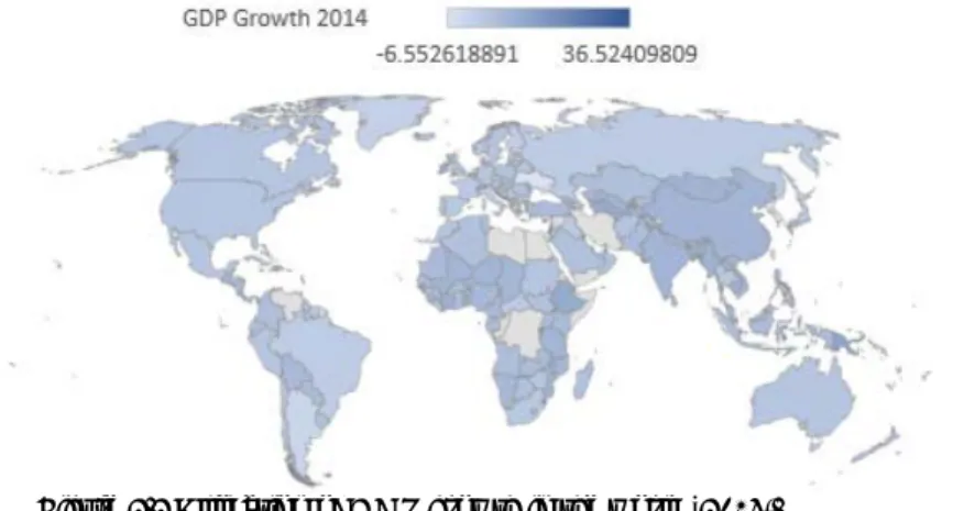
Figure 2.3 Allocation of GDP growth in the world (2014). ... 6

Tables

Table 4.1 Variables used on the regression model ... 15

Table 5.1 Modelling GDP growth on its determinants ... 21

Table 5.2 Results of Granger causality tests on income groups 1996-2015 ... 22

Appendices

Appendix B – Augmented Dickey-Fuller unit root test ... 31

Appendix C – Correlation matrix ... 32

Appendix D – Redundant fixed effects test ... 33

Appendix E – Hausman test... 34

Appendix F – Wald´s test ... 35

1

Introduction

____________________________________________________________________________________

This chapter provides the reader with the motivation and purpose of the topic chosen, as well as an overview of method and main results.

______________________________________________________________________ Two of the most well-known researchers analysing economic growth, Romer (1990) and Solow (1957), both conclude that long-run growth is driven by nothing except technological change. This technical change derives from investments in research and development (R&D), in which R&D being the creation or improvement of new goods or alterations of production strategies to increase efficiency. Researchers such as Grossman and Helpman (1994), Lhuillery and Miotti (2008) and Sørensen (1997) establish a relation among R&D and economic performance. Although researchers can ascertain a relationship, it is less straight-forward to interpret the empirical results due to the issue of endogeneity. The endogeneity problem regards the question whether R&D causes economic growth or economic growth causes R&D. Knowing that there is a relationship among R&D and GDP growth, one might expect the direction of causality among high-income economies and low-income economies to be different. This can further be connected to the so-called R&D paradox, meaning that countries with the largest R&D expenditure are not always the ones growing the most rapidly, indicating that after a certain threshold it demands more for an economy to grow (Brown & Svensson, 1988; Hall & Oriani, 2006; Minniti & Venturini, 2017). However, studies investi-gating the causality between R&D and GDP growth on income classifications in the world, have been somewhat overlooked in more recent years, meaning that countries might overin-vest in their R&D expenditure if it can be concluded that GDP growth causes the amount of R&D investments.

It is therefore of interest to investigate the endogeneity problem further using short-term and long-term tests of Granger causality. Our study aims not only to confirm the relation of R&D and GDP growth but rather to shed new light on the issue of endogeneity, among countries with different income levels. However, this thesis differs from the studies men-tioned above in multiple ways. This study is conducted on a world level, dividing the coun-tries into income groups, thus not only including more councoun-tries but also focusing on a

dif-which is rarely occurring in previous studies. Hence the purpose is twofold, firstly we estab-lish if R&D is related to economic growth, by investigating the following research question: Does the level of R&D expenditure have a positive relationship with economic growth over time? Secondly, we investigate whether R&D Granger causes gross domestic product (GDP) growth or vice versa between countries with diverse levels of income, since one would expect the Granger causality to be different among the different income groups, by asking: How does the Granger causality between R&D expenditure and GDP growth look like among countries with various income levels?

To answer these research questions, the econometric analysis is based on a sample of 60 countries with different income levels around the world between 1996-2015. The first re-search question is tested by different model specifications, including: capital, labour, R&D, trade and corruption, the appropriate model specification is thereafter applied to a fixed ef-fects model (FEM) to establish a relation among GDP growth and R&D. Thereafter, the sample is divided into different sub-samples according to the income classification provided by the World Bank. These income classifications are as follows: high-income, upper-middle-income, and lower-middle-income. Low-income is excluded due to lacking data availability. The second research question is investigated by conducting a Granger causality test and Jo-hansen’s cointegration test in combination with the Toda-Yamamoto augmented Granger causality test on the different income levels, to determine the direction of Granger causality among R&D expenditure and GDP growth.

By carrying out a FEM one can conclude a positive relationship among R&D growth and economic performance during the 20 years investigated. However, conducting a Wald’s test confirms that the R&D variable is endogenous, meaning that the FEM is not appropriate for estimating or testing and even less forecasting. This leads us to the second research question, which specifically addresses the issue of endogeneity. A Granger causality test is conducted, indicating how the growth of R&D influences GDP growth in the short-run for all income levels in the sample. However, the Toda-Yamamoto augmented Granger causality test indi-cates that the direction of Granger causality among the regarded variables is unestablished in the long-run regardless of income level. This suggests conflicting results for the long-run test, since the Johansen's cointegration test, performed in combination with the Toda-Yama-moto approach, indicates cointegration between the variables in the long-run, meaning that these two tests contradict each other.

The structure of the paper is therefore as follows: Section 2 - Background, provides the reader

with an overview of relevant statistics and figures regarding R&D spending in different coun-tries and different income levels. Section 3 – Previous Research, discusses endogenous growth

theory, which is fundamental for the analysis. Moreover, previous empirical findings are sum-marised. Section 4 - Empirical Framework, provides a thorough description of the

methodol-ogy used and the empirical model. Moreover, diagnostics tests and robustness tests are touched upon. And lastly, Granger causality tests, testing both short run and long run are considered. Section 5 - Empirical Results and Analysis, presents results and analyses these,

connecting back to the previous research. Section 6 - Conclusion, summaries the paper,

stresses importance of certain aspects for society and science and concludes with limitations and suggested future research.

2 Background

___________________________________________________________________________________

This chapter presents basic facts and figures regarding R&D expenditure in different countries.

_____________________________________________________________________ The world´s R&D expenditure as percentage of GDP does not depict a straight upward trend (seen in figure 2.1), rather it has varied from a minimum of 1.95 percent of GDP to a maximum of 2.23 percent of GDP between the years 1996-2015. First in 2007 the world experienced a sustained upward trend in R&D spending as a share of GDP, due to the level of R&D expenditure growing more rapidly than GDP (World Bank, 2018a). Although the overall spending of R&D as a percentage of GDP increases in the world, the geographical allocation portrays a highly unequal picture (see figure 2.2), not only among high-income economies and lower-income economies but one can further observe discrepancies among high-income economies themselves.

Analysing the average R&D spending as a percentage of GDP of each of the individual countries in the sample, one can conclude that Europe, Asia and the United States are in the front edge of R&D expenditure relative to GDP (see appendix A). Additionally, from the sample one can confirm the differences in R&D spending as a percentage of GDP among the high-income economies, this becomes especially apparent considering Trinidad and To-bago which has an average R&D spending of 0.079 percent of GDP compared to United States which has an average R&D spending of 2.661 percent of GDP. In the upper-middle-income category, China, Brazil and Russia stand out due to their relatively high values, each with an average R&D spending as a percentage of GDP of 1.481, 1.072, 1.120. These are

1,9 1,95 2 2,05 2,1 2,15 2,2 2,25 1996 1998 2000 2002 2004 2006 2008 2010 2012 2014 %

Figure 2.1 R&D expenditure (% of GDP) in the world (1996-2015). (Source: The World Bank, 2018a)

part of BRIC, which symbolises fast growing economies (UN News, 2017). In the lower-middle-income economies only two countries stand out, this is Ukraine and India, with av-erage R&D expenditure as a percentage of GDP of 0.881 and 0.771, respectively. India is moreover a BRIC member. Other countries in the lower-middle-income group have an av-erage R&D expenditure as a percentage of GDP ranging from 0.093 to 0.422. From table 2.1, providing an outlook of descriptive statistics for the three income groups in the sample, one can observe the highest mean spending on R&D in the high-income group, followed by upper-middle-income and lastly lower-middle-income.

Comparing figure 2.2 displaying the allocation of R&D expenditure relative to GDP in the world, with figure 2.3 portraying GDP growth in all countries, one can observe a contrasting picture. Countries with higher R&D expenditure relative to GDP do not show to be the ones growing the most rapidly. This picture is maybe not what one would expect, rather one would expect countries spending more on R&D to grow faster, meaning that R&D would Granger cause GDP growth whereas for lower-income economies one might expect GDP growth to Granger cause R&D (Goni & Maloney, 2014). Countries that spend the most on R&D do not grow as much as the ones spending less, depicting the R&D paradox.

Table 2.1 Descriptive statistics for income groups during 1996-2015

GDP Growth (%) R&D GDP Growth (%) R&D GDP Growth (%) R&D GDP Growth (%) R&D Mean 0.3622 16.800 0.3271 25.000 0.1962 7.8600 0.7172 3.9500 Median 0.0639 1.2000 0.0518 3.3900 0.0884 0.5470 0.0917 0.0629 Maximum 151.05 506.00 151.05 506.00 43.341 229.00 88.560 49.100 Mimimum -0.9992 0.0009 -0.9992 0.0006 -0.9974 0.0009 -0.9637 0.0031 Std.dev 5.4755 53.100 6.0561 67.800 2.2891 24.600 7.6195 9.1600 R&D values are in billions U.S. dollar

Descriptive Statistics R&D and GDP Growth 1996-2015

All Income Groups High-Income Upper-Middle-Income Lower-Middle-Income

The same pattern can be observed regarding the sample of the paper, looking at the descrip-tive statistics on R&D expenditure and GDP growth in table 2.1. Comparing income groups, one can conclude that the high-income group has the highest mean R&D expenditure in absolute terms, however, one can additionally observe that it does not have the highest mean GDP growth. The lowest mean GDP growth can be observed for the upper-middle-income group even though they spend more on R&D in absolute terms than the lower-middle-in-come group. The inlower-middle-in-come group growing the most but also spending the least on R&D in absolute terms is the lower-middle-income group, thus somewhat confirming the R&D par-adox. However, also bear in mind that less wealthy economies might portray higher GDP growth rates due to reasons other than simply the R&D paradox, for instance increasing capital accumulation, leading to above normal growth rates (Solow, 1956).

Figure 2.3 Allocation of GDP growth in the world (2014). (Source: The World Bank, 2018b)

Figure 2.2 Allocation of R&D expenditure (% of GDP) in the world (2014).

This relates to the catch-up effect and the marginal returns to economic growth. Emerging countries generally have a higher marginal return to GDP growth than developed economies, meaning that poorer countries experience a more rapid increase in economic growth since every input used in production is more productive than for higher-income economies. This also implies that developed economies will reap relatively less benefits from adding one extra unit of input (capital and labour) into production, meaning that they will observe a threshold level concerning economic growth (Solow, 1956). More recent studies agree upon a similar argument, that R&D becomes less of an important input in production the wealthier an economy is, meaning that one can observe a threshold level also within the R&D sector (Lederman & Maloney, 2003; Minniti & Venturini, 2017).

Another explanation to the R&D paradox put forward by UNESCO (2015) is how initiatives in R&D are mostly conducted by the private sector. This indicates a converging trend, where high-income economies spend less on R&D in the public sector, whereas the private sector has either grown or maintained. Moreover, high-income economies invest in R&D to stay competitive in the global market. The same cannot be concluded for lower-income econo-mies, rather one can observe increasing investments in R&D on a public level, used as a growth strategy to improve economic performance. What UNESCO (2015) concludes for all income groups are that they strive to have the most talented researchers which leads to investments in higher education and research laboratories. Private firms, on the other hand, can easier reallocate research infrastructure to benefit from countries with labour-intensive populations, meaning that lower-income economies reap the largest benefits from produc-tion. When countries, on all income levels, invest in researchers and public R&D, this in-crease the initiative for the private sector to tap into R&D. Although, private and public initiatives in R&D have different targets, economic growth depends on how well they com-plement each other (UNESCO, 2015).

3 Previous Research

____________________________________________________________________________________

This chapter provides relevant theories regarding economic growth and presents the hypotheses tested in this study.

______________________________________________________________________

3.1 Growth Theory

Solow (1956) brings forward one of the first mathematically derived growth models, stressing the importance of capital and labour accumulation. Furthermore, Solow (1957) makes the substantial conclusion that long-run growth is driven by nothing except technological pro-gress. However, the model does not conclude what drives the technological progress, thus technology is exogenous. Romer (2012) argues that the endogenous growth model was de-veloped as a response to consider economic growth further. The main difference between the endogenous growth model and the Solow model is how technology is treated, in which the first defines four microeconomic factors that determines the level of R&D, compared to Solow's model in which it is exogenous.

Romer (1990) presents an endogenous growth model, with the idea of R&D being motivated by private profits from innovation, which in turn increase the incentives to further invest-ment in R&D. The model assumes that knowledge consists of dissimilar ideas and are there-fore imperfect substitutes. An additional assumption made is monopoly rights for the devel-oper, excluding others from using the idea, hence also allowing for temporary monopoly profits. Moreover, capital is excluded since it complicates the model´s implications due to transition dynamics, meaning that the economy does not move directly to its new balanced growth route. Hence, the exclusion of capital simplifies the calculation and the analysis of the model´s main points. On the other hand, when including capital, analyses can be con-ducted on the distribution of output among investment and consumption due to policies, which is not possible in the previous scenario. However, since the model´s main purpose is the same, both including or excluding capital, the most efficient choice is to exclude it. With this simplification, the model’s key equation is:

𝑌𝑌̇(𝑡𝑡)

𝑌𝑌(𝑡𝑡) = max{

(1 − ø)2

∅ 𝐵𝐵𝐿𝐿� − (1 − ∅)𝜌𝜌, 0}

(Equation 1)

Equation 1 explains how, (𝑌𝑌̇(𝑡𝑡)

𝑌𝑌(𝑡𝑡)), the growth rate of the growth rate of output (the acceleration

rate) is determined by four microeconomic factors. Firstly, discount rates (𝜌𝜌) affectthe num-ber of employees devoted to R&D since a higher interest leads to less patient employees and less investment in R&D (due to opportunity costs). Secondly, substitutability among the inputs used in R&D itself (ø). The higher the degree of substitutability the less workers en-gaged in R&D, in combination with slower productivity growth since in this case each input contributes less to output. Thirdly, the productivity of R&D (B), has a positive relation to growth. In addition, an increase in the productivity of R&D raises the willingness for workers to engage in that sector. Finally, an increase in population size (𝐿𝐿�) automatically raises eco-nomic growth in the long-run since the model assumes that all individuals are engaged in either the production of intermediate inputs or in the production of R&D. Consequently, the number of employees devoted to R&D production is assumed to increase as the size of the population raises. Moreover, this also enlarge the returns to R&D since the larger the economy the more extended the market is for R&D, increasing its returns. In brief, all these microeconomic factors affect the number of workers devoted to R&D which in turn deter-mines economic long-term growth.

However, the Romer model possesses certain drawbacks, firstly, by presuming only linear growth, and secondly, suggesting how advancements in R&D are merely an upsurge in the amount of inputs used in the production. Therefore, one might consider applying models put forward by Aghion and Howitt (1990), Grossman and Helpman (1991) as well as Jones (1995). Jones (1995) proposed a model permitting transition dynamics, thus the driving fac-tor for growth in the long run is solely the growth rate of population. Aghion and Howitt (1990) and Grossman and Helpman (1994) alter how the technology process is defined, ar-guing how enhancements of prevailing inputs represent innovations. However, due to its simplicity, the regression in this thesis is based on Romer´s endogenous growth model (see equation 1), which furthermore, is the most well-known theory regarding R&D´s

contribu-On the other hand, other researchers find evidence of economic growth being the driving force of R&D which contradicts Romer´s model (see the next section, 3.2, for other re-searchers’ findings). Romer (1990) places less focus on the possibility of GDP growth being a determinant of R&D expenditure instead of vice versa, implying that Romer´s model is of more importance examining our first research question (see section 3.3).

3.2 Related Literature

Previous research has diverse opinions on what is the predominant driver of economic growth. Capital accumulation and labour have been regarded as the most crucial factors in-fluencing economic performance (Solow, 1957). Most researchers also stress the significance of technological change for improved living standards and economic development (Gross-man & Help(Gross-man, 1994; Romer 1986, 1990; Solow, 1957). Investments in technology, specif-ically R&D, do not only benefit the private investor but the society as whole (Grossman & Helpman, 1994). Sørensen (1997) extends the argumentation by arguing that occasionally it is of relevance to subsidise areas such as R&D and education since these might result in economic growth. More recent studies from Huang and Lin (2006) as well as Raffo, Lhuillery and Miotti (2008) stress how knowledge inputs, specifically R&D, generally yield improve-ments in innovation, and thus impact economic growth positively. However, worth noticing is that the amount of R&D documented is merely a portion of what is spent on investments of new methods and goods, which therefore should be considered (Evenson & Westphal, 1995). Lastly, factors that might influence the level of R&D investments and economic growth more than policies and innovations are: institutions, laws, economic environment and mobility (Evenson & Westphal 1995; Grossman & Helpman, 1994; Pack & Westphal, 1986).

R&D investments are proved to have various outcomes despite the same amount invested, meaning that there is no simple model how to make R&D efficient (Pisano, 2012). Pisano (2012) also argues that the underlying mechanisms behind successful R&D investments are: the combination of the amount of labour and the level of skilled labour devoted to different production groups, the capacity and the headquarter of the R&D production, the technology

used in the creation of R&D as well as the distribution of resources. Moreover, Pisano (2012) emphasises that companies do not perform equally well at all the components required for a profitable R&D investment, meaning that they all should have different strategies to increase R&D efficiency. This might be an explanation to why countries with different income levels experience various returns from R&D investments. For instance, Sørensen (1997) stresses that accumulation of education and skills should be the main priority when human capital is below a certain level. It is first after passing this hurdle it is beneficial for innovative activities and R&D, relating back to Pisano´s (2012) argumentation about the importance of skilled labour engaged in the R&D process.

Moreover, Sørensen (1997) concludes that less developed countries receive advantages of an open economy, due to technology spill overs. Grossman and Helpman (1994) highlight that a country should export the good in which they have a comparative advantage in, therefore countries with high human capital will have a head start in technology and will consequently export these goods in exchange for labour-intensive goods and for goods that do not demand the newest technology. These findings enlighten the importance of the type of technology used in the R&D production as well as the value of a company's geographical location, in theory with Pisano´s (2012) findings. This indicates that unequally wealthy countries should have different production strategies to R&D, due to their diverse specialization of industries. However, not everyone agrees that R&D causes economic growth. Birdsall and Rhee (1993) conclude that it is not R&D that affects economic growth rather it is the vice versa. Further-more, Bresnahan (1986) and Mansfield et al. (1977) argue that the amount of investments in commercial R&D is too small to impact economic performance. Moreover, R&D is proved to becomes less of a significant contributor to economic growth when a region possesses more advanced technology. Hence, R&D (as a factor of economic growth) is a non-linear function of already existing use of technology within a firm (Minniti & Venturini, 2017). Lederman and Maloney (2003) support this argumentation and stress that developing econ-omies are mostly favoured of R&D returns. In addition, Brown and Svenson (1988) stress how managers generally do not measure their returns on R&D expenditure, in fear of

receiv-reasonable motives. This view is supported by Hall and Oriani (2006), concerning developed economies, arguing that European companies too rarely value its R&D investments.

3.3 Hypotheses

Summing up previous literature, providing different opinions regarding R&D´s impact on economic growth, brings motivation to the following hypothesis for research question 1:

 _{R&D positively relates to GDP growth}

This hypothesis is tested by equation 3, presented in the empirical framework.

However, whether it is R&D that Granger causes GDP growth, or the other way around in different income classifications, is ambiguous, hence we test the following hypothesis for research question 2:

 The Granger causality among R&D and economic growth is different in countries with diverse income levels

This is tested by a Granger causality test and a Johansen's cointegration test in combination with the Toda-Yamamoto augmented Granger causality test (see equation 5, 6, 7 & 8).

4 Empirical Framework

_____________________________________________________________________________________

The purpose of this chapter is to give a clear overview of: the data, model specifications and diagnostic tests and robustness tests.

______________________________________________________________________

4.1 Data

To investigate the proposed research questions data is gathered for the period 1996-2015 for a sample of 60 countries belonging to different income groups (see appendix A). This sample is collected allowing for five missing data points between 1996-2015 per variable and per country. The reason for allowing for five missing data points is a level effect in the R&D and corruption variables, meaning that countries either have approximately five missing data points or approximately ten missing data points, the lower alternative is therefore more ap-propriate. Moreover, the missing values is kept empty, meaning that we have an unbalanced panel data. Countries are thereafter divided into subsamples based on their income level, according to the income classification provided by the World Bank (2018c). The total sample of countries are, accordingly, divided into the following categories: high-income countries, upper-middle-income countries and lower-middle-income countries. Due to lacking data availability low-income countries are excluded from the analysis. These categories are based on the gross national income (GNI) per capita in current U.S. dollar, in which economies having a GNI per capita between $1,006-$3,955 are classified as lower-middle-income coun-tries, economies with GNI per capita of $3,956-$12,235 are upper-middle-income countries and economies exceeding $12,235 being classified as high-income economies.

The main data source used is the World Bank, providing statistics for the variables in the production function: capital, labour and R&D, as well as the control variable trade. However, the World Bank does not provide information regarding the level of corruption within a country and therefore to obtain data for the Corruption Perception Index (CPI) Transpar-ency International (The Global Anti-Corruption Coalition) is used.

4.2 Variables in the Econometric Analysis

To establish what drives economic growth, it is of relevance to establish which factors that have a significant relationship to it. As Solow (1957) concludes, it is not only capital and labour that are related to growth. The dependent and the independent variables are presented and justified below and a summary of the variables and how they are defined can be found in table 5.1.

GDP. To investigate what drives economic development (see equation 2 & 3), GDP growth

is the dependent variable in the data set. It is established by market prices measured in the domestic currency and converted to U.S. dollar (The World Bank, 2018d).

Capital. Measured by gross capital formation, is based on the economy´s expenses on

amend-ments regarding the fixed assets together with net alterations in the degree of inventories (The World Bank, 2018e).

Labour. Refers to individuals, of age 15 and above, supplying labour in production of goods

and services. It considers both individuals employed and those searching for employment (The World Bank, 2018f).

R&D. Is the sum of public and private investment initiatives in innovating activities in

tech-nology as well as culturally and socially (World Bank, 2018a).

Trade Openness. Is the summation of goods and services being exported and imported, measured as a percentage of GDP (World Bank, 2018g). By specialising and exporting the goods and services in which a country has a comparative advantage, it will improve the coun-try's economic performance (Grossman & Helpman, 1994).

Corruption. Here measured by CPI, ranks countries in the world from 0 (highly corrupt) to 10

(no corruption being present) based on the estimated level of corruption in the public sector. The ranking is based on opinions from: residents, experts within the field and outstanding observers (Transparency International, 2018). One would expect institutions and laws to

positively affect economic growth (Evenson & Westphal, 1995; Grossman & Helpman, 1994; Pack & Westphal, 1986).

4.3 Empirical Model of R&D´s Relation to GDP Growth

The data is plotted to validate a linear relationship among the variables. To control for ex-treme outliers a robustness test, using winsorization, is conducted on all the variables before the model is specified. Winsorization is conducted at the 0.5% level, meaning that outliers above or below the 0.5th percentile are removed to receive the value of the 99.5th percentile. Moreover, White´s cross-section standard errors and covariance is used to regard potential problems with heteroscedasticity within the cross-sections, which furthermore is applied for all models estimated. In addition, all regressions are tested at the 5% significance level.

Table 4.1 Variables used on the regression model

Description Abbreviation

Dependent Variable

GDP growth GDP (Current US$) ∆lnGDP

Transformed by taking the natural logarithm and thereafter taking the first difference to correct for non-stationarity

Independent Variable Expected Impact

Labour growth (%) Total labour force glnL +

Transformed by taking the natural logarithm and thereafter converting it into a percentage growth rate to correct for non-stationarity

Capital growth (%) Gross capital formation (Current US$) glnC + Transformed by taking the natural logarithm and thereafter converting

it into a percentage growth rate to correct for non-stationarity

R&D growth Research and development expenditure (% of GDP) ∆lnR&D + Transformed by taking the natural logarithm of the absolute value and

thereafter taking the first difference to correct for non-stationarity

Trade openess Trade (% of GDP) lnTO +

Transformed by taking the natural logarithm

CPI Corruption Perception Index CPI

-See appendix B for ADF unit root test on variables

4.3.1 Model Specifications

The Solow Growth model provides a fundamental basis in economic development theories, and hence, provides a starting point for the analysis. Therefore, the first model includes only the variables capital and labour in explaining economic performance. However, non-station-ary variables have time-vnon-station-arying mean and/or variance meaning that they are improper for forecasting. Hence the unit root test Augmented Dickey Fuller (ADF) test is conducted on the variables. This results in capital and labour being converted into percentage growth rates.

∆𝑙𝑙𝑙𝑙𝑙𝑙𝑙𝑙𝑙𝑙𝑖𝑖𝑡𝑡 = 𝛼𝛼1+ 𝛽𝛽1𝑔𝑔𝑙𝑙𝑙𝑙𝑔𝑔𝑖𝑖𝑡𝑡+ 𝛽𝛽2𝑔𝑔𝑙𝑙𝑙𝑙𝐿𝐿𝑖𝑖𝑡𝑡+υ𝑖𝑖𝑡𝑡

(Equation 2)

To extend equation 2 further towards Romer´s (1990) proposition of R&D and technology as a significant factor to economic growth, R&D as well as two control variables: trade and corruption are added. Furthermore, an ADF test indicates undesirable patterns in the varia-bles trade and R&D, while corruption is stationary in its original form (see appendix B for unit root tests on all variables). Therefore, the variables GDP and R&D are transformed to growth rates by taking the first difference, lastly, trade is replaced by trade openness. This does not only correct for non-stationarity but also for multicollinearity, which otherwise would have been present among R&D and trade in absolute terms (see appendix C for cor-relation matrix).

∆𝑙𝑙𝑙𝑙𝑙𝑙𝑙𝑙𝑙𝑙𝑖𝑖𝑡𝑡 = 𝛳𝛳1+ 𝛿𝛿1𝑔𝑔𝑙𝑙𝑙𝑙𝑔𝑔𝑖𝑖𝑡𝑡+ 𝛿𝛿2𝑔𝑔𝑙𝑙𝑙𝑙𝐿𝐿𝑖𝑖𝑡𝑡+ 𝛿𝛿3∆𝑙𝑙𝑙𝑙𝑙𝑙&𝑙𝑙𝑖𝑖𝑡𝑡+ 𝛿𝛿4𝑙𝑙𝑙𝑙𝑙𝑙𝑙𝑙𝑖𝑖𝑡𝑡+ 𝛿𝛿5𝑔𝑔𝑙𝑙𝐶𝐶𝑖𝑖𝑡𝑡+ε𝑖𝑖𝑡𝑡

(Equation 3)

Equation 3 is adjusted and tested using a pooled ordinary least squares (OLS), random effects model (REM) and a FEM. To determine the appropriate model, one tests the pooled OLS and FEM against each other using a redundant fixed effects test. Rejecting the null hypoth-esis, H0: Pooled OLS is appropriate, one can conclude that FEM is preferable (see appendix D). Furthermore, a Hausman test is conducted to conclude whether a FEM or a REM is appropriate. Moreover, this test additionally concludes that FEM is preferable, thus rejecting the null hypothesis of REM being the appropriate model (see appendix E). Thus, the FEM is specified as follows:

∆𝑙𝑙𝑙𝑙𝑙𝑙𝑙𝑙𝑙𝑙𝑖𝑖𝑡𝑡 = 𝜇𝜇1+ 𝜆𝜆1𝑔𝑔𝑙𝑙𝑙𝑙𝑔𝑔𝑖𝑖𝑡𝑡+ 𝜆𝜆2𝑔𝑔𝑙𝑙𝑙𝑙𝐿𝐿𝑖𝑖𝑡𝑡+ 𝜆𝜆3∆𝑙𝑙𝑙𝑙𝑙𝑙&𝑙𝑙𝑖𝑖𝑡𝑡+ 𝜆𝜆4𝑙𝑙𝑙𝑙𝑙𝑙𝑙𝑙𝑖𝑖𝑡𝑡+ 𝜆𝜆5𝑔𝑔𝑙𝑙𝐶𝐶𝑖𝑖𝑡𝑡+ν𝑡𝑡+ 𝜔𝜔𝑖𝑖+ 𝜂𝜂𝑖𝑖𝑡𝑡 𝑖𝑖 = 𝑐𝑐𝑐𝑐𝑐𝑐𝑙𝑙𝑡𝑡𝑐𝑐𝑐𝑐 1,2, … ,60 𝑡𝑡 = 𝑡𝑡𝑖𝑖𝑡𝑡𝑡𝑡 1996, 1997, … ,2015 ν𝑡𝑡= 𝑐𝑐𝑡𝑡𝑦𝑦𝑐𝑐 𝑑𝑑𝑐𝑐𝑡𝑡𝑡𝑡𝑖𝑖𝑡𝑡𝑑𝑑 𝜔𝜔𝑖𝑖= 𝑐𝑐𝑐𝑐𝑐𝑐𝑙𝑙𝑡𝑡𝑐𝑐𝑐𝑐 𝑑𝑑𝑠𝑠𝑡𝑡𝑐𝑐𝑖𝑖𝑠𝑠𝑖𝑖𝑐𝑐 𝑠𝑠𝑖𝑖𝑓𝑓𝑡𝑡𝑑𝑑 𝑡𝑡𝑠𝑠𝑠𝑠𝑡𝑡𝑐𝑐𝑡𝑡 (Equation 4)

The FEM holds both cross-sections (countries) and period (time) fixed, meaning that the slope coefficients are equal across countries, but with different intercepts which varies over time (Gujarati & Porter, 2009).

4.4 Empirical Model of Causality

For the FEM to be unfaltering all explanatory variables need to be exogenous. As depicted in appendix F, the R&D variable is not exogenous when conducting a Wald´s test, meaning that there are problems with endogeneity in the independent variable R&D, causing the FEM to be less useful for estimating and especially inappropriate in forecasting (Gujarati & Porter, 2009). To consider this, a Granger causality test and the Toda-Yamamoto approach in com-bination with Johansen's cointegration test are conducted.

Granger (1969) emphasises the relevance of the direction of causality among variables exam-ined. Even though a significant relationship can be established among the variables it does not prove the direction of the causality between them. The basic intuition behind the Granger causality test is that if one occurrence befalls before another, the initial event may influence the latter, but not vice versa (see equation 5 and 6). This test assumes the variables to be stationary and error terms to be uncorrelated. However, transforming non-stationary variables by taking the first difference deteriorate the long-term relation among the regarded variables (Granger, 1969). Further drawbacks are non-validity concerning non-linear and in-stantaneous relationships. Also, seasonality effects can cause misinterpretation of causality if they are not considered. For instance, public holidays such as Christmas, is the reason to why

hold (Granger, 1979). Moreover, the Granger causality test requires the variables to be inte-grated of the same order. Since, the variables R&D and GDP are in their first difference, the variables fulfil the criterion of same integration order, in this case integrated of order one. Furthermore, Schwarz criterion and Akaike information criteria are used to determine the optimal lag length for each individual income group. However, since this test is incapable of measuring the long-term relationship between two variables, it is only used for examining the short-run influence.

∆𝑙𝑙𝑙𝑙𝑙𝑙𝑙𝑙𝑙𝑙𝑡𝑡= � 𝛼𝛼𝑖𝑖 𝑛𝑛 𝑖𝑖=1 ∆𝑙𝑙𝑙𝑙𝑙𝑙&𝑙𝑙𝑡𝑡−𝑖𝑖+ � 𝛽𝛽𝑗𝑗∆𝑙𝑙𝑙𝑙𝑙𝑙𝑙𝑙𝑙𝑙𝑡𝑡−𝑗𝑗 𝑛𝑛 𝑗𝑗=1 + 𝑐𝑐1𝑡𝑡 (Equation 5) ∆𝑙𝑙𝑙𝑙𝑙𝑙&𝑙𝑙𝑡𝑡= � 𝜆𝜆𝑖𝑖∆𝑙𝑙𝑙𝑙𝑙𝑙&𝑙𝑙𝑡𝑡−𝑖𝑖+ � 𝛿𝛿𝑗𝑗∆𝑙𝑙𝑙𝑙𝑙𝑙𝑙𝑙𝑙𝑙𝑡𝑡−𝑗𝑗+ 𝑐𝑐2𝑡𝑡 𝑛𝑛 𝑗𝑗=1 𝑛𝑛 𝑖𝑖=1 (Equation 6)

Where ΔlnGDP is the first difference of absolute GDP in natural logarithm, ΔlnR&D is the first difference of absolute R&D expenditure in natural logarithm (see table 4.1), i and j is the optimal lag lengths and the u is an error term.

Toda and Yamamoto (1995) enlarge the Granger causality testing by bringing forth an ap-proach that is appropriate regardless of whether the data is stationary, non-stationary (and not cointegrated) or cointegrated. The test is built on a vector autoregressive (VAR) model based on the levels of the data regarded, meaning that the data is run in its original form (see equation 7 and 8). The number of lags included is determined from information criteria, which furthermore, is required to be extended by one additional lag to examine whether the model is dynamically stable. This approach is based on Granger causality; however, it does not deteriorate any long-term relationship suggesting a useful complement to the original Granger causality test. Hence, to regard the longer direction of Granger causality the Toda-Yamamoto approach is exercised. Moreover, for the Toda-Toda-Yamamoto´s Granger causality results to be equivalent to Johansen's cointegration test, the variables must exhibit a signifi-cant direction of Granger causality and simultaneously be cointegrated, or be insignifisignifi-cant with no cointegration present, otherwise there is a substantial indication of conflicting results.

Since this approach has no restrictions regarding order of integration, one does not have to correct the variables for non-stationarity for this test to be valid, hence the variables are tested in their original form.

∆𝑙𝑙𝑙𝑙𝑙𝑙𝑡𝑡= 𝛼𝛼 � 𝛽𝛽𝑖𝑖∆𝑙𝑙𝑙𝑙𝑙𝑙𝑡𝑡−𝑖𝑖+ � 𝛾𝛾𝑗𝑗𝑙𝑙&𝑙𝑙𝑡𝑡−𝑗𝑗+ 𝑐𝑐𝑦𝑦𝑡𝑡 𝑘𝑘+𝑑𝑑 𝑗𝑗=1 ℎ+𝑑𝑑 𝑖𝑖=1 (Equation 7) 𝑙𝑙&𝑙𝑙𝑡𝑡= 𝛼𝛼 + � 𝜃𝜃𝑖𝑖𝑙𝑙&𝑙𝑙𝑡𝑡−1 ℎ+𝑑𝑑 𝑖𝑖=1 + � 𝛿𝛿𝑗𝑗∆𝑙𝑙𝑙𝑙𝑙𝑙𝑡𝑡−𝑗𝑗+ 𝑐𝑐𝑥𝑥𝑡𝑡 𝑘𝑘+𝑑𝑑 𝑗𝑗=1 (Equation 8)

Where ΔGDP is the first difference of the absolute GDP (since the purpose is to examine the relation of R&D expenditure and GDP growth, and not R&D expenditure´s relation to GDP in absolute terms), R&D expenditure is in absolute terms, h and k are the optimal lag lengths of GDP growth and R&D, d is the maximal order of integration and u is an error term, assumed to be white noise.

4.4.1 Additional Diagnostic Tests and Robustness Tests

A Jarque-Bera normality test is conducted to detect undesirable patterns in the residuals. Conducting this normality test for all income groups, one can conclude that the residuals are non-normally distributed for the high-income group and the upper-middle-income group. Whereas, for the lower-middle-income the residuals are normally distributed (see appendix G for all normality tests).

5 Empirical Results and Analysis

_____________________________________________________________________________________

The purpose of this chapter is to provide the reader with an extensive analysis regarding R&D relation to economic growth and in which direction the causality exists.

______________________________________________________________________

5.1 Analysis of R&D´s Relation to GDP Growth

To investigate the first research question a FEM is conducted on equation 3, symbolising (3) in table 5.1. Thus, table 5.1 depicts outcomes for the aggregated panel regression for the timespan 1996-2015. The Durbin-Watson statistic is rather close to two, meaning that most likely there are no problems with autocorrelation. Analysing the fundamental variables capital and labour one can observe immense discrepancies, capital growth is statistically significant whereas labour growth is insignificant for all models, meaning that capital growth relates to the expansion in GDP whereas, labour growth does not. Capital has long been known to be the main source to economic growth (Solow 1956, 1957), hence the positive significant result is expected. The control variable corruption has the expected sign; however, it is not signif-icant at the 5% significance level when controlling for period and cross-section in the FEM, on the other hand, observing the standard errors one can conclude that it is not far from significance. The control variable trade openness has a negative effect on GDP growth in the FEM.

Lastly, focusing on the R&D variable, the FEM indicates that growth in R&D expenditure has a positive relationship to economic growth when aggregating all countries in the sample, which is supported by Grossman & Helpman, (1994), Romer (1986, 1990) and Solow, (1957). This aspect is additionally touched upon by more recent studies (Huang & Lin, 2006; Raffo, Lhuillery & Miotti, 2008). However, the coefficient of R&D in the FEM is 0.001609 percent, implying that R&D growth has a relatively small relationship to economic development, on the other hand, the true value of R&D investment is only a small fraction of all investment initiatives taken regarding new development (Evenson & Westphal, 1995). This could be an explanation to the relatively low coefficient of the R&D variable. On the other hand, since R&D growth is not strongly (or even weakly) exogenous, these results are generally not fully accurate, meaning that it is not of relevance to extend this model further, or applying it on the different income groups. However, this enlightens the importance of our second research

Table 5.1 Modelling GDP growth on its determinants Independent Variables (2) (3) Intercept 0.0014* 0.0122* (0.0001) (0.0121) Capital growth 0.3658* 0.3580* (0.0104) (0.0121) Labour growth 0.0418 0.0675 (0.1032) (0.1038) R&D growth - 0.0016* (0.0006) Trade openess - -0.0021* (0.0007) CPI - -0.0003 (0.0002) Nr. of observations 1198 956 Durbin-Watson 1.8944 1.8168 R-squared 0.7494 0.7676 * indicates that p-value < 0.05

Standard errors in parenthesis, estimated using White´s cross-section standard errors and covariance estimator

FEM Modeling GDP Growth on its Determinants

5.2 Analysis of Causality

One can conclude that R&D growth Granger causes GDP growth for all income levels dur-ing the time span 1996-2015 usdur-ing the Granger causality test (see table 5.2). This test repre-sents the short-term relationship, implying that R&D growth is a determinant of economic growth in the short-run regardless of income level. This result is rather unexpected, since one would expect GDP growth to influence growth in R&D expenditure in lower-middle-income countries due to less wealthy economies (Goni & Maloney, 2014). However, the results for the two remaining income groups, high-income and upper-middle-income are as expected, stressing that R&D growth Granger causes GDP growth (Romer, 1990). Further-more, UNESCO (2015) emphasises how lower-income economies and middle-income econ-omies invest in R&D in an attempt to create a sustainable strategy for growth to raise income levels and better the welfare, while, high-income economies invest mostly in R&D to stay competitive on the global market.

However, these empirical results might illuminate the so-called R&D-paradox, meaning that developed countries tend to invest in R&D regardless of the final outcomes, on account of, partly national policies (public R&D) but predominantly private R&D investments (Brown & Svenson, 1988; Hall & Oriani, 2006). On the other hand, this does not mean that R&D is not providing higher-income countries with productive advantages, simply that less wealthy countries are catching up, receiving relatively larger benefits of its R&D expenditure, which is supported by UNESCO (2015) presented in the background chapter. In short, even though one can observe a direction of Granger causality from R&D growth to economic growth, one cannot measure to what extent it is profitable to invest in R&D, meaning that high-income economies might overinvest in R&D compared to what is efficient.

Table 5.2 Results of Granger causality tests on income groups 1996-2015

R&D Granger GDP growth Granger Nr. of obs. R&D Granger causes GDP growth Granger Nr. of obs. GDP growth causes R&D GDP growth causes R&D

All Income Levels 7E-15* 0.6487 968 0.0649 0.7227 528 High-Income 2E-7* 0.1025 546 0.1021 0.3221 438 Upper-Middle-Income 6E-5* 0.8464 306 0.1326 0.2531 170 Lower-Middle-Income 4E-3* 0.6737 116 0.6692 0.7345 102 * indicates that p-value < 0.05

Values displayed are p-values

Short Run (Granger causality) Long Run (Toda-Yamamoto approach) Granger causality and Toda-Yamamoto Granger causality on different income groups

Further explanations to the results can be based on firms´ choice of location, indicating the importance of the different production strategies to obtain efficient R&D investments, among different countries (Pisano, 2012). For instance, multinational firms choose to invest in R&D in high-income countries but the production itself is accomplished in countries with less expensive capital and labour force, meaning that those countries reap the predominant benefits of R&D investment. This is supported by Grossman and Helpman (1994) and UNESCO (2015). Grossman and Helpman (1994) enlighten the basics behind trade theory, essentially countries should export what they have a comparative advantage in. Higher-in-come economies usually have knowledge-intensive advantages and hence invest in R&D whereas lower-income countries generally possess labour-intensive advantages resulting in the production of the inventions. This also relates to the level of education among different countries. Lower-income economies generally have less educated populations indicating that they should have a different approach to increase their R&D profitability (Pisano, 2012). As Sørensen (1997) argues it should be a main priority to invest in human capital since it is first after the lower-income economies have reached a sufficiently high level of education that it is beneficial for them to invest in R&D. However, in our results we can observe that R&D growth Granger causes GDP growth also for the lower-middle-income group, indicating that this income group has either a sufficiently educated population or benefits from technology spill overs from more developed economies.

Furthermore, when considering the Toda-Yamamoto augmented Granger causality test one cannot observe the direction of the relationship in the period 1996-2015. This approach considers the long-term, implying that the direction of Granger causality among R&D ex-penditure and economic growth is unestablished. This result contradicts the results expected, believing that R&D investment would be a determinant in economic growth for the high-income and upper-middle-high-income countries and vice versa regarding the lower-middle-in-come group. However, worth mentioning is that when considering the Granger causality for all income groups aggregated, the p-value is close to significant (approximately 0.06),

mean-Moreover, we have a conflict in the results in all income levels in which Johansen's cointe-gration test indicates cointecointe-gration between the variables, meaning that one should observe a Granger causality between the variables in at least one direction, however, the Toda Yama-moto procedure does not indicate any long-run relationship. These contradicting results may rise from our relatively short time span, which deteriorates the test´s reliability (Toda and Yamamoto, 1995) or since some of the p-values are relatively close to significance, it implies that the Toda-Yamamoto approach might not have conflicting results with Johansen's coin-tegration test testing at a higher significance level i.e. 10%.

6 Conclusion

_____________________________________________________________________________________

This chapter summarises the paper with focus on the main findings, the limitations of the analysis con-ducted, contributions to society and future research possibilities.

______________________________________________________________________ The purpose of this paper is to firstly, investigate whether R&D is positively related to GDP growth, and thereafter, analyse the direction of this relationship in different income levels, looking at Granger causality in the short-run as well as the long-run. This is conducted using panel data consisting of 60 countries over a period of 20 years, from 1996-2015. The data is mainly collected from the World Bank, however, Transparency International (The Global Anti-Corruption Coalition) is also used.

The results in this paper display a positive relationship between GDP growth and the growth of R&D expenditure, using a FEM allowing for country specific intercepts varying over time. The strength of their relationship is somewhat lower than expected, with a possible explana-tion of R&D being only a fracexplana-tion of all initiatives taken in creaexplana-tion of new goods and meth-ods. Furthermore, the R&D variable seems to be endogenous in the model, meaning that whether R&D growth drives economic growth or vice versa is less straightforward. The Granger causality tests show, however, that on short-term basis, the growth of R&D ex-penditure has a positive impact on GDP growth regardless of income level. One might have expected GDP growth to Granger cause R&D growth for the lower-middle-income group due to its inferior economic benchmark. A reasonable motivation to this might be the un-derlying mechanisms behind efficient R&D, for instance, where multinational corporations choose to geographically place their production, since this influence where the benefits of R&D are ultimately reaped. Further explanations can be the level of educated people within different income groups, meaning that they face different strategies to increase R&D produc-tivity. Moreover, considering the long-run results no clear conclusion can be ascertained to whether it is R&D expenditure that Granger causes economic development or vice versa. Conflicts between Johansen's cointegration test and the Toda-Yamamoto procedure exist,

conflicting results might be the length of the time span, meaning that it might not be long enough for what is required for the Toda-Yamamoto approach to provide credible results. R&D growth is, in this paper, proved to Granger cause economic growth in the short run irrespective of income level. This implies that R&D adds value to a country's economic de-velopment regardless of whether countries are classified as developed or emerging, meaning that also lower-middle-income economies benefit from investments in R&D. The dimen-sions of the R&D-paradox are still unrequited, meaning that it is difficult to measure if de-veloped countries overinvest or efficiently deposit capital in R&D. Despite the ambiguities, R&D investments stimulate economic growth and should, to some extent, be favoured by policy regardless of a nation's level of development.

A limitation of the study is the data availability of R&D expenditure as a percentage of GDP, not only for individual countries but also for the timespan, in which only 1996-2015 is avail-able. As data collection develops one can exploit all income levels and hence, future research-ers can utilise the better data availability and therefore develop studies regarding R&D in countries with lower income. Moreover, as time progresses the time span investigated could be extended and can therefore better account for the long-term effects of R&D. Another limitation is that inflation is not accounted for in the model. Moreover, savings is not con-sidered in the regression when modelling GDP growth on its determinants, due to its lacking data availability.

Suggestions for future research studies are, to investigate which underlying factors that cause R&D productivity and therefore GDP growth. Moreover, it would be of interest to combine R&D with policies and regulations in for instance an interaction term and thus, investigate whether different policies and regulations of dissimilar countries cause a multiplier effect of R&D on GDP growth.

Reference list

Aghion, P., & Howitt, P. (1990). A model of growth through creative destruction (Research Report

No. 3223). Retrieved from the NBER: http://www.nber.org/pa-pers/w3223.pdf

Birdsall, N., & Rhee, C. (1993). Does results and development (R&D) contribute to economic growth in developing countries? (Research Report No. 1221). Retrieved from the World

Bank:

http://documents.worldbank.org/cu-rated/en/666031468780281251/pdf/multi0page.pdf

Bresnahan, T. F. (1986). Measuring the spillovers from technical advance: mainframe com-puters in financial services. The American Economic Review, 76(4), 742-755.

Re-trieved from http://web.b.ebscohost.com.proxy.li- brary.ju.se/ehost/pdfviewer/pdfviewer?vid=1&sid=d3af3dc4-ed33-4089-a139-9751f7d29925%40sessionmgr120

Brown, M. G., & Svenson, R. A. (1988). Measuring r&d productivity. Research-Technology Man-agement, 31(4), 11-15. https://doi.org/10.1080/08956308.1988.11670531

Evenson, R. E., & Westphal, L. E. (1995). Technological change and technology strategy.

Handbook of development economics, 3, 2209-2299.

https://doi.org/10.1016/S1573-4471(05)80009-9

Goni, E., & Maloney, W. F. (2014). Why don´t poor countries do R&D? (Research Report No.

6811). Retrieved from the World Bank: http://documents.worldbank.org/cu-rated/en/855681468326185477/Why-dont-poor-countries-do-R-D

Granger, C. W. (1969). Investigating causal relations by econometric models and cross-spec-tral methods. Econometrica: Journal of the Econometric Society, 37(3), 424-438. doi:

10.2307/1912791

Granger, C.W. (1979). Seasonality: Causation, Interpretation, and Implications. In A. Zellner (Ed.), Seasonal Analysis of Economic Time Series (pp. 33-56). Retrieved from

NBER.

Grossman, G. M., & Helpman, E. (1991). Innovation and growth in the global economy. Cambridge:

MIT press.

Grossman, G. M., & Helpman, E. (1994). Endogenous innovation in the theory of growth.

Journal of Economic Perspectives, 8(1), 23-44. doi: 10.1257/jep.8.1.23

Gujarati, N. D. & Porter, C. D. (2009a). Basic Econometrics (5th _{ed.). New York: McGraw-Hill}

International Journal of Industrial Organization, 24(5), 971-993.

https://doi.org/10.1016/j.ijindorg.2005.12.001

Huang, E. Y., & Lin, S. C. (2006). How R&D management practice affects innovation per-formance: An investigation of the high-tech industry in Taiwan. Industrial

Man-agement & Data Systems, 106(7), 966-996.

https://doi.org/10.1108/02635570610688887

Jones, C. I. (1995). R & D-based models of economic growth. Journal of political Economy, 103(4), 759-784. https://doi.org/10.1086/262002

Lederman, D., & Maloney, W. (2003). R&D and development. (Research Report No. 3024).

Retrieved from the World Bank: http://documents.worldbank.org/cu-rated/en/778751468739477640/pdf/multi0page.pdf

Mansfield, E., Rapoport, J., Romeo, A., Wagner, S., & Beardsley, G. (1977). Social and private rates of return from industrial innovations. The Quarterly Journal of Economics, 91(2), 221-240. https://doi.org/10.2307/1885415

Minniti, A., & Venturini, F. (2017). R&D policy, productivity growth and distance to frontier.

Economics Letters, 156, 92-94. https://doi.org/10.1016/j.econlet.2017.04.005

Pack, H., & Westphal, L. E. (1986). Industrial strategy and technological change: theory ver-sus reality. Journal of development economics, 22(1), 87-128.

https://doi.org/10.1016/0304-3878(86)90053-2

Pisano, G. P. (2012). Creating an R&D Strategy. (Research Report No. 12-095). Retrieved from

Harvard Business School: https://www.hbs.edu/faculty/Publica-tion%20Files/12-095_fb1bdf97-e0ec-4a82-b7c0-42279dd4d00e.pdf

Raffo, J., Lhuillery, S., & Miotti, L. (2008). Northern and southern innovativity: a comparison across European and Latin American countries. The European Journal of Develop-ment Research, 20(2), 219-239. https://doi.org/10.1080/09578810802060777

Romer, D. (2012). Advanced Macroeconomics (4th ed.). New York: McGraw-Hill Education.

Romer, P. M. (1986). Increasing returns and long-run growth. Journal of political economy, 94(5),

1002-1037. https://doi.org/10.1086/261420

Romer, P. M. (1990). Endogenous technological change. Journal of political Economy, 98(5), 71-102. https://doi.org/10.1086/261725

Solow, R. M. (1956). A contribution to the theory of economic growth. The quarterly journal of economics, 70(1), 65-94. https://doi.org/10.2307/1884513

Solow, R. M. (1957). Technical change and the aggregate production function. The review of Economics and Statistics, 39(3), 312-320. doi:10.2307/1926047

The World Bank. (2018a). Research and development expenditure (% of GDP). Retrieved February

10th_{, 2018, from}

https://data.worldbank.org/indica-tor/GB.XPD.RSDV.GD.ZS

The World Bank. (2018b). GDP growth (annual %). Retrieved February 8th_{, 2018, from}

https://data.worldbank.org/indicator/NY.GDP.MKTP.KD.ZG

The World Bank. (2018c). World Bank Country and Lending Groups. Retrieved 1st _{April, 2018,}

from https://datahelpdesk.worldbank.org/knowledgebase/articles/906519-world-bank-country-and-lending-groups

The World Bank. (2018d). GDP (Current US$). Retrieved February 20th_{, 2018, from}

https://data.worldbank.org/indicator/NY.GDP.MKTP.CD

The World Bank. (2018e). Gross capital formation (Current US$). Retrieved February 20th_{, 2018,}

from https://data.worldbank.org/indicator/NE.GDI.TOTL.ZS

The World Bank. (2018f). Labor force, total. Retrieved March 8th_{, 2018, from}

https://data.worldbank.org/indicator/SL.TLF.TOTL.IN

The World Bank. (2018g). Trade (% of GDP). Retrieved February 26th _{February, 2018, from}

https://data.worldbank.org/indicator/NE.TRD.GNFS.ZS

Toda, H. Y., & Yamamoto, T. (1995). Statistical inference in vector autoregressions with possibly integrated processes. Journal of econometrics, 66(1), 225-250.

https://doi.org/10.1016/0304-4076(94)01616-8

Transparency International. (2018). FAQs on Corruption. Retrieved February 20th_{, 2018, from}

https://www.transparency.org/whoweare/organisation/faqs_on_corrup-tion/9

United Nations Educational, Scientific and Cultural Organization (UNESCO). (2015).

UNESCO Science Report: towards 2030 – Executive Summary. Retrieved from

http://unesdoc.unesco.org/images/0023/002354/235407e.pdf

United Nations (UN). (2017, June 16). 'BRICS' countries well placed to help lead global ef-forts to tackle hunger – UN agency. UN News. Retrieved from

https://news.un.org/en/story/2017/06/559662-brics-countries-well-placed-help-lead-global-efforts-tackle-hunger-un-agency

Appendices

Appendix A – Country list with income groups and average R&D expenditure

Country list per income group with average R&D expenditure (%)

(Source: The World Bank, 2018a)

Austria 2.500 Korea, Rep. 3.142 Argentina 0.494 Armenia 0.249 Belgium 2.044 Lithuania 0.802 Azerbaijan 0.243 Egypy, Arab Rep. 0.413 Canada 1.879 Latvia 0.540 Bulgaria 0.543 India 0.771 Cyprus 0.378 Netherlands 1.819 Belarus 0.674 Kyrgyz Republic 0.177 Czech Republic 1.394 Norway 1.626 Brazil 1.072 Moldova 0.422 Germany 2.601 Poland 0.687 China 1.481 Tajikistan 0.093 Denmark 2.708 Portugal 1.105 Colombia 0.185 Ukraine 0.881 Spain 1.161 Singapore 2.115 Cuba 0.496 Uzbekistan 0.238 Estonia 1.251 Slovak Republic 0.641 Ecuador 0.243

Finland 3.355 Slovenia 1.803 Croatia 0.857 France 2.140 Sweden 3.389 Kazakhstan 0.208 United Kingdom 1.639 Trinidad and Tobago 0.079 Mexico 0.446 Greece 0.656 Uruguay 0.335 Macedonia, FYR 0.287 Hungary 1.070 United States 2.661 Panama 0.219 Ireland 1.325 Romania 0.438 Iceland 2.531 Russian Federation 1.120 Israel 4.102 Serbia 0.661 Italy 1.162 Thailand 0.300 Japan 3.178 Turkey 0.702

Average R&D Expenditure (% of GDP) per Country With Countries Divided According to Income Levels

Lower-Middle-Income Upper-Middle-Income

Appendix B – Augmented Dickey-Fuller unit root test H0: Unit root (non-stationary)

H1: No unit root (stationary)

A ugm ente d D ick ey F ulle r u nit r oot te st o n v aria bles Be fo re c o rre c tio n M e thod S ta ti sti c P rob. S ta ti sti c P rob. S ta ti sti c P rob. S ta ti sti c P rob. S ta ti sti c P rob. S ta ti sti c P rob. A D F - F is h e r Ch i-s q u a re 146. 165 0. 0403 100. 466 0. 9020 102. 364 0. 8761 85. 3057 0. 9930 51. 3302 1. 0000 207. 556 0. 0000 A D F - Ch o i Z -s ta t 1. 25703 0. 8956 1. 79575 0. 9637 3. 29355 0. 9995 4. 85327 1. 0000 6. 52091 1. 0000 -4. 91826 0. 0000 A ft e r c o rre c tio n M e thod S ta ti sti c P rob. S ta ti sti c P rob. S ta ti sti c P rob. S ta ti sti c P rob. S ta ti sti c P rob. A D F - F is h e r Ch i-s q u a re 181. 721 0. 0002 330. 941 0. 0000 376. 040 0. 0000 291. 917 0. 0000 172. 487 0. 0012 A D F - Ch o i Z -s ta t -4. 17100 0. 0000 -9. 89178 0. 0000 -10. 1114 0. 0000 -8. 25889 0. 0000 -2. 13854 0. 0162 A ll v a ria b le s a re in n a tu ra l lo g a rit h m s A ugm e nt e d D ic ke y-F ul le r U ni t R oot T e st R& D R & D gr ow th T ra de T ra de ope ne ss C or rupt ion GD P G D P gr ow th C ap ital C a pi ta l gr ow th ( % ) L a bour L a bour gr ow th ( % )

Appendix C – Correlation matrix

Correlation matrix of variables in regressions

ΔlnGDP glnC glnL lnR&D ΔlnR&D lnT lnTO CPI

ΔlnGDP 1 0.8202 0.1310 -0.2108 0.3013 -0.1732 0.0769 -0.2147 glnC 0.8202 1 0.1346 -0.1534 0.2613 -0.1261 0.0645 -0.1468 glnL 0.1310 0.1346 1 -0.1027 0.0759 -0.0571 -0.0144 0.0259 lnR&D -0.2108 -0.1534 -0.1027 1 -0.1300 0.9299 -0.3207 0.5435 ΔlnR&D 0.3013 0.2613 0.0759 -0.1300 1 -0.1057 0.0306 -0.1201 lnT -0.1732 -0.1261 -0.0571 0.9299 -0.1057 1 -0.2173 0.4998 lnTO 0.077 0.0645 -0.0144 -0.3207 0.0306 -0.2173 1 0.1474 CPI -0.2147 -0.1468 0.0259 0.5435 -0.1201 0.4998 0.1474 1

Appendix D – Redundant fixed effects test H0: Pooled OLS is preferred

H1: Pooled OLS is not preferred (FEM is appropriate)

Redundant fixed effects test determining whether pooled OLS or FEM is appropriate.

Test cross-section and period fixed effects

Effects Test Statistic d.f. Prob.

Cross-section F 1.0996 -59.884 0.2874 Cross-section Chi-square 68.4841 59 0.1865 Period F 14.4692 -18.884 0.0000 Period Chi-square 249.6969 18 0.0000 Cross-Section/Period F 3.9339 -77.884 0.0000 Cross-Section/Period Chi-square 284.9275 77 0.0000 Redundant Fixed Effects Test

Appendix E – Hausman test H0: REM is preferred

H1: REM is not preferred (FEM is appropriate)

Hausman test determining whether REM or FEM is appropriate.

Test period random effects

Test Summary Chi-Sq. Statistic Chi-Sq. d.f. Prob.

Period random 28.9598 5 0.0000

Appendix F – Wald´s test

H0: No endogeneity (exogenous)

H1: Endogeneity

Wald´s test of endogeneity on R&D growth

Test Statistic Value df Probability

t-statistic 2.5799 884 0.0100 F-statistic 6.6557 (1, 884) 0.0100

Chi-square 6.6557 1 0.0099

Appendix G – Jarque-Bera normality test H0: Normally distributed residuals

H1: Non-normally distributed residuals

Jarque-Bera normality test for high-income group 1996-2015.

Jarque-Bera normality test for upper-middle-income group 1996-2015.